The Kinematic and Static Analysis of the Tibio-Femoral Joint Based on a Novel Spatial Mechanism

Abstract

To reveal the characteristics of knee movement and tibio-femoral joint contact force, a novel single degree of freedom spatial mechanism is built to simulate the joint kinematics based on a three dimensional model of the human knee. The length changes of the three ligaments can be obtained by establishing and solving the kinematics spiral function. Based on this mechanism, a static model is built where linear springs are used to model the ligaments and whose stiffness coefficients are obtained by the finite element method. The main strength of the proposed model is that it associates the knee's flexion motion with internal/external rotation of the tibia based on the isometricity of the anterior cruciate ligament. This offers an efficient method to model and analyse the changes of ligament lengths and static kinematics after ligament reconstruction, which is crucial in designing knee recovery and rehabilitation equipment.

1. Introduction

The knee is the largest and the most complex joint in the human body, whose function is providing the fundamental support for body movements. However, due to direct exposure, the joint components such as the anterior cruciate ligament (ACL), are easily injured which might lead to joint instability and movement changing, and even disability. The structure/kinematics characteristics of the knee are a key problem in knee joint rehabilitation or reconstruction surgery.

Recently, the analysis of the movement of knee joint has become a hot topic. Due to the knee's complexity, the mechanism theory is gradually used to simulate the joint motion. O'Connor [1] proposed a planar four-bar linkage in sagittal plane to analyse the knee movement, where the anterior cruciate ligament (ACL) and the posterior cruciate ligament (PCL) were assumed to be isometric and their positions on the tibia and femur were joint centres. It had significant value in analysing the knee motion and the interaction forces between the ligament and muscle, and also developing a machine to restore knee functions. Later, Wilson and O'Connor [2] proposed a novel equivalent spatial mechanism with a single degree of freedom. The anterior cruciate ligament (ACL), posterior cruciate ligament (PCL) and medial collateral ligament (MCL) were considered as links, each ligament connected to the tibia and femur with a spherical and a universal joint. The medial and lateral condyles of femur are modelled as spheres and the tibia condyles as planar surfaces, the contact between the femur and tibia condyle are single point of frictionless contacts. In [3–6], Wilson et al. improved the tibial condyle planes in the ESM-1 mechanism into more anatomically-shaped surfaces by substituting the femur and tibia in ESM-1 with two spheres (ESM-2) and general shape surfaces (ESM-3). The results of the models were in better agreement with experiments when more anatomically-shaped surfaces were applied.

Knowing the kinematics of the tibio-femoral joint is of importance to analysing the joint contact force and decreases the possibility of ligament, menisci and articular cartilage trauma. The paper presents a novel spatial mechanism to simulate the knee kinematics and quasi-static analysis after ACL reconstruction.

2. Material and Methods

2.1 Construct the spatial mechanism of tibio-femoral joint

2.1.1 Extract the characteristic structure and feature points of the tibio-femoral joint

The three dimensional model of the tibio-femoral joint was built in MIMICS software based on the computer tomography (CT) and magnetic resonance images (MRI) from a volunteer. The surface processing was done in Geomagic Studio software including Boolean operations, geometry registering, image registration and NURBS surfaces generating. Then a three dimensional model of the tibio-femoral joint (Fig. 1) was obtained including femur, tibia, fibular and articular cartilages, and four ligaments which are the anterior cruciate ligament (ACL), the posterior cruciate ligament (PCL), the medial collateral ligament (MCL) and the lateral collateral ligament (LCL).

Figure 1.

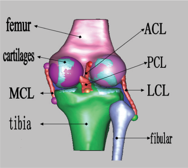
The feature elements on the tibio-femoral joint

According to the observations by Amis [7], the fibres within ACL could be considered isometric during the knee flexion. In the proposed model, the ACL is represented by a link – the starting and ending points of the link is the intersection points between ligaments and bones as depicted as points, the distance between the two points is the length of ACL. As in [8], the posterior femoral condyles were close to spheres, the two circular posterior femoral condyles are modelled as two spheres, the axis penetrating through the two spherical centres (called the flexion facet centres, FFC) was defined as a rotation feature line of the femur. The tibio-femoral contact point was defined as the feature point on the tibia medial condyle.

2.1.2 Spheres fitting on circular posterior femoral condyles

After constructing the spatial mechanism of the tibiofemoral joint, regression algorithms are used to solve the rotation line of the femur. Let P₀(x₀,y₀,z₀) be the centre of the sphere, r be the radius of the sphere, the spherical equation can be expressed as:

${(\mathbf{x}-{\mathbf{x}}_0)}^2+{(\mathbf{y}-{\mathbf{y}}_0)}^2+{(\mathbf{z}-{\mathbf{z}}_0)}^2={\mathbf{r}}^2$

(1)

Twenty points on the posterior femoral condyles' surface were selected, of which the position vector is defined as A_i(x_i,y_i,z_i), (i = 1,2,…,20). In line with the least squares principle, the residual error denoted by f could be expressed as:

$\mathbf{f}={\displaystyle \sum _{\mathbf{i}=1}^n{[{({\mathbf{x}}_{\mathbf{i}}-{\mathbf{x}}_0)}^2+{({\mathbf{y}}_{\mathbf{i}}-{\mathbf{y}}_0)}^2+{({\mathbf{z}}_{\mathbf{i}}-{\mathbf{z}}_0)}^2-{\mathbf{r}}^2]}^2}$

(2)

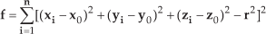
simplified as:

$\mathbf{f}={\displaystyle \sum _{\mathbf{i}=1}^n{[-2{\mathbf{x}}_{\mathbf{i}}{\mathbf{x}}_0-2{\mathbf{y}}_{\mathbf{i}}{\mathbf{y}}_0-2{\mathbf{z}}_{\mathbf{i}}{\mathbf{z}}_0+\mathbf{R}+{\mathbf{b}}_{\mathbf{i}}]}^2}$

(3)

where R and b_i is expressed as:

$\{\begin{array}{l}\mathbf{R}={\mathbf{x}}_0{}^2+{\mathbf{y}}_0{}^2+{\mathbf{z}}_0{}^2-{\mathbf{r}}^2\\ {\mathbf{b}}_{\mathbf{i}}={\mathbf{x}}_{\mathbf{i}}{}^2+{\mathbf{y}}_{\mathbf{i}}{}^2+{\mathbf{z}}_{\mathbf{i}}{}^2\begin{array}{cc}& \end{array}\end{array}$

the position of sphere centres, as well as the radius of each sphere can be obtained as the least squares solution of Equation (3). The results show that the radius of the medial condyle fit sphere is 21.34 mm and that of the lateral condyle is 23.04 mm, which is in agreement with the results in [7] (the radius of the medial sphere is about 22 mm and that of the lateral sphere 24 mm).

2.1.3 Build the spatial mechanism of the tibio-femoral joint

• 1)

  Feature elements of the ligaments

  In the normal tibio-femoral joint, the ACL is modelled as a link which is connected to the femur and tibia by spherical (S) and universal (U) joints respectively. The other three ligaments, MCL, LCL and PCL, are modelled as two links, each of which is connected by a prismatic (P) joint, and each two link is connected to the femur and tibia by spherical (S) and universal (U) joints respectively.

• 2)

  Feature elements of the femur and tibia

  Both the femur and tibia are defined as circular planes. The revolute (R) joint on the femur is defined by the rotation feature line. Another revolute (R) joint on the tibia is set by the axis across the contact point and perpendicular to the tibia condyle.

The spatial mechanism was constructed as presented in Fig. 2. However, both the femur and tibia have the relative rotation to the global frame. In order to simplify the process of solving the kinematics equations, an equivalent link was defined to maintain the same motion when the global frame was built on the tibia (tibial fixed frame). The final spatial mechanism is shown in Fig.3.

Figure 2

The spatial mechanism with global frame

Figure 3

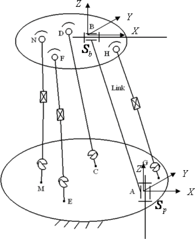
The spatial mechanism with tibial fixed frame.

Table 1.

Coordinates of feature points measured in global fixed frame XYZ.

Feature point	x/mm	y/mm	z/mm
D (starting point of ACL on femur)	86.61	93.76	0.79
C (Ending point of ACL on tibia)	82.23	80.54	−24.17
A (contact point on tibia medial condyle)	112.21	81.26	−29.56
B (centre of medial condyle sphere)	116.28	88.78	−3.80
B' (centre of lateral condyle sphere)	64.06	97.93	−2.64
F (starting point of PCL on femur)	103.75	95.19	−7.42
E (ending point of PCL on tibia)	88.49	114.55	−35.49
M (starting point of MCL on femur)	132.94	85.50	−4.79
N (ending point of MCL on tibia)	125.01	82.72	−45.56
H (starting point of LCL on femur)	50.86	106.67	1.68
G (ending point of MCL on fibular)	35.17	119.18	−65.77

2.2 Kinematics analysis of the spatial mechanism

The moving coordinate system denoted by S_p is established on the tibia where the origin point is represented by A (contact point on medial tibia condyle), while the static coordinate system denote by S_b is established on the femur where the origin point is represented by B (centre of medial condyle sphere). The two coordinate systems are parallel to each other, where the x-axis is parallel to the rotation feature line, y-axis is defined perpendicular to the coronal plane, z-axis is established by right hand rule. A single degree of freedom can be obtained for the mechanism and then screw theory is used to solve the forward kinematics. The product of exponential formula is expressed as:

${\mathbf{g}}_{\mathbf{s}\mathbf{t}}={\mathbf{e}}^{{\widehat{\xi }}_{11}{\theta }_{11}}\cdots {\mathbf{e}}^{{\widehat{\xi }}_{1n_{{}_1}}{\theta }_{1n_{{}_1}}}{\mathbf{g}}_{\mathbf{s}\mathbf{t}}(0)=\cdots ={\mathbf{e}}^{{\widehat{\xi }}_{\mathbf{i}1}{\theta }_{\mathbf{i}1}}\cdots {\mathbf{e}}^{{\widehat{\xi }}_{\mathbf{i}\mathrm{j}}{\theta }_{\mathbf{i}\mathbf{j}}}{\mathbf{e}}^{{\widehat{\xi }}_{\mathbf{i}\text{j+1}}{\theta }_{\mathbf{i}\mathbf{j}+1}}\cdots {\mathbf{e}}^{{\widehat{\xi }}_{\mathbf{i}{n}_{{}_{\mathbf{i}}}}{\theta }_{\mathbf{i}{n}_{{}_{\mathbf{i}}}}}{\mathbf{g}}_{\mathbf{s}\mathbf{t}}(0)$

(4)

where i and j are the number of branch chain and number of joint in branch chain, ξ _ij denotes the spinor of the jth joint in the ith branch chain, θ _ij denotes the displacement of the jth joint in ith branch chain, g_st denotes the configuration matrix and g_st(0) represents the initial configuration of the femur relative to the tibia.

Five motion screws were chosen in AB and CD branch chain, expressed as:

$\begin{array}{l}{\xi }_{11}={(\begin{array}{cc}-{\omega }_{11}\times {\mathbf{r}}_{\mathbf{A}}& {\omega }_{11}\end{array})}^T\\ {\xi }_{12}={(\begin{array}{cc}-{\omega }_{12}\times {\mathbf{r}}_{\mathbf{B}}& {\omega }_{12}\end{array})}^T\\ {\xi }_{21}={(\begin{array}{cc}-{\omega }_{21}\times {\mathbf{r}}_{\mathbf{C}}& {\omega }_{21}\end{array})}^T\\ {\xi }_{22}={(\begin{array}{cc}-{\omega }_{22}\times {\mathbf{r}}_{\mathbf{C}}& {\omega }_{22}\end{array})}^T\\ {\xi }_{23}={(\begin{array}{cc}-{\omega }_{23}\times {\mathbf{r}}_{\mathbf{D}}& {\omega }_{23}\end{array})}^T\end{array}$

where ω _ij represents the vector axis of the jth joint in the ith branch chain (i=1,2; j=1,2,3), r_A, r_B, r_C and r_D denote positions of point A, B, C and D relative to space coordinate system. So

$\begin{array}{l}{\mathbf{g}}_{\mathbf{s}\mathbf{t}}={\mathbf{e}}^{{\widehat{\xi }}_{11}{\theta }_{11}}{\mathbf{e}}^{{\widehat{\xi }}_{12}{\theta }_{12}}{\mathbf{g}}_{\mathbf{s}\mathbf{t}}(0)\\ \begin{array}{cc}& =\left[\begin{array}{cc}{\mathbf{R}}_1& 0\\ 0& 1\end{array}\right]\end{array}\left[\begin{array}{cc}{\mathbf{R}}_2& {\mathbf{p}}_1\\ 0& 1\end{array}\right]\left[\begin{array}{cc}\mathbf{I}& {\mathbf{r}}_{\mathbf{B}}\\ 0& 1\end{array}\right]\\ \begin{array}{cc}& =\left[\begin{array}{cc}{\mathbf{R}}_1{\mathbf{R}}_2& {\mathbf{R}}_1{\mathbf{R}}_2{\mathbf{r}}_{\mathbf{B}}+{\mathbf{R}}_1{\mathbf{p}}_1\\ 0& 1\end{array}\right]\end{array}\end{array}$

(5)

where, ${\mathbf{R}}_1=\left[\begin{array}{ccc}\mathbf{c}{\theta }_{11}& -\mathbf{s}{\theta }_{11}& 0\\ \mathbf{s}{\theta }_{11}& \mathbf{c}{\theta }_{11}& 0\\ 0& 0& 1\end{array}\right]$ , ${\mathbf{R}}_2={\mathbf{e}}^{{\widehat{\omega }}_{12}{\theta }_{12}}$ , ${\mathbf{p}}_1=(\mathbf{I}-{\mathbf{e}}^{{\widehat{\omega }}_{12}{\theta }_{12}}){\mathbf{r}}_{\mathbf{B}}$ , $\mathbf{c}{\theta }_{11}=\mathrm{c}\mathrm{o}\mathrm{s}{\theta }_{11}$ , $\mathbf{s}{\theta }_{11}=\mathrm{s}\mathrm{i}\mathrm{n}{\theta }_{11}$ , ACL is modelled as rigid link, the length denotes by δ, we can get

$\{\begin{array}{l}\Vert {\mathbf{q}}_{\mathbf{D}}^{\mathbf{p}}-{\mathbf{q}}_{\mathbf{C}}^{\mathbf{p}}\Vert =\delta \\ {\mathbf{q}}_{\mathbf{D}}^{\mathbf{p}}={\mathbf{g}}_{\mathbf{s}\mathbf{t}}{\mathbf{q}}_{\mathbf{D}}^{\mathbf{b}}\begin{array}{c}\end{array}\end{array}$

(6)

where q^p_D and q^p_C represent the homogenous coordinates of point D and C measured in static coordinate system S_p and q^b_D represents homogenous coordinate of point D measured in moving coordinate system S_b. The Equation (6) could be simplified as

$\Vert {\mathbf{R}}_1({\mathbf{R}}_2{\mathbf{q}}_{\mathbf{D}}+{\mathbf{R}}_2{\mathbf{r}}_{\mathbf{B}}+{\mathbf{p}}_1)-{\mathbf{r}}_{\mathbf{C}}\Vert =\delta$

(7)

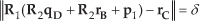
Now the Equation (7) becomes the sub-problem of Paden-Kahan 3 problem in [9], where the θ₁₁ and R ₁ could be solved by the corresponding method in [9], then g_st could be solved in (5). After getting the θ₁₁, the kinematic characteristics of other joints could be solved by the inverse kinematics method of the parallel robot. Finally, the length of ligaments is represented as:

$\{\begin{array}{c}{\mathbf{l}}_{\mathbf{L}\mathbf{C}\mathbf{L}}=\Vert {\mathbf{g}}_{\mathbf{s}\mathbf{t}}{\mathbf{q}}_{\mathbf{M}}^{\mathbf{b}}-{\mathbf{q}}_{\mathbf{N}}\Vert \\ {\mathbf{l}}_{\mathbf{P}\mathbf{C}\mathbf{L}}=\Vert {\mathbf{g}}_{\mathbf{s}\mathbf{t}}{\mathbf{q}}_{\mathbf{F}}^{\mathbf{b}}-{\mathbf{q}}_{\mathbf{E}}\Vert \\ {\mathbf{l}}_{\mathbf{M}\mathbf{C}\mathbf{L}}=\Vert {\mathbf{g}}_{\mathbf{s}\mathbf{t}}{\mathbf{q}}_{\mathbf{H}}^{\mathbf{b}}-{\mathbf{q}}_{\mathbf{G}}\Vert \end{array}$

(8)

where q^b_M q^b_F and q^b_H are the positions of points M, F and N measured in moving coordinate system S_b; q_N, q_E and q_G are the positions of points N, E and G measured in static coordinate system S_p.

2.3 Static analysis of the tibio-femoral joint after ACL reconstruction

2.3.1 Length and equivalent elastic coefficient of ligaments

Each ligament, except ACL, is modelled as a linear spring. The three-dimensional model of each ligament is meshed in ANSYS software and then analysed as shown in Fig. 4. Ligaments are considered as isotropic material and elastic modulus of PCL is 276 MPa, MCL is 292 MPa, and LCL is 292 MPa, the Poisson-ratio is 0.49 for all three ligaments [12]. Then the elastic coefficient is calculated using the finite element method, PCL is 192.85 N/mm, that of MCL is 260.55 N/mm and for LCL is 29.03 N/mm and the initial force are then calculated which are 125.01N/mm, 125.01 N/mm and 209.83 N respectively for PCL, MCL and LCL.

Figure 4

Finite element model of ligaments. (a). PCL, (b). MCL, (c) LCL

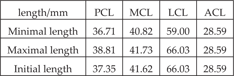
It is well-recognized by most scholars that the ligaments cannot resist compress forces. It is supposed that the ligaments will not receive any compressive forces during knee flexion. The minimal length of each ligament during flexion is considered as the original length, the original length and maximal length is obtained by the forward kinematics solution, the initial length is measured as the knee is at complete extension (Table 2).

Table 2

The length of ligaments

length/mm	PCL	MCL	LCL	ACL
Minimal length	36.71	40.82	59.00	28.59
Maximal length	38.81	41.73	66.03	28.59
Initial length	37.35	41.62	66.03	28.59

2.3.2 Static kinematics simulation of the tibio-femoral joint

The femur is selected to analyse the force of each ligament (Fig. 5), force and moment balance equations are expressed as:

${\overrightarrow{\mathbf{F}}}_{\mathbf{F}}+{\overrightarrow{\mathbf{F}}}_{\mathbf{N}}+{\overrightarrow{\mathbf{F}}}_{\mathbf{D}}+{\overrightarrow{\mathbf{F}}}_{\mathbf{H}}+{\overrightarrow{\mathbf{F}}}_{\mathbf{B}}=0$

(9)

${\overrightarrow{\mathbf{r}}}_{\mathbf{B}\mathbf{F}}\times {\overrightarrow{\mathbf{F}}}_{\mathbf{F}}+{\overrightarrow{\mathbf{r}}}_{\mathbf{B}\mathbf{N}}\times {\overrightarrow{\mathbf{F}}}_{\mathbf{N}}+{\overrightarrow{\mathbf{r}}}_{\mathbf{B}\mathbf{D}}\times {\overrightarrow{\mathbf{F}}}_{\mathbf{D}}+{\overrightarrow{\mathbf{r}}}_{\mathbf{B}\mathbf{H}}\times {\overrightarrow{\mathbf{F}}}_{\mathbf{H}}+{\overrightarrow{\mathbf{M}}}_{\mathbf{B}}=0$

(10)

Figure 5

Model of quasi-static kinematics

where ${\overrightarrow{\mathbf{F}}}_{\mathbf{F}}\mathrm{,}\hspace{0.17em}{\overrightarrow{\mathbf{F}}}_{\mathbf{N}}\mathrm{,}\hspace{0.17em}{\overrightarrow{\mathbf{F}}}_{\mathbf{D}}\mathrm{,}\hspace{0.17em}{\overrightarrow{\mathbf{F}}}_{\mathbf{H}}$ and ${\overrightarrow{\mathbf{F}}}_{\mathbf{B}}$ denote the forces on point F, N, D, H and B respectively, ${\overrightarrow{\mathbf{r}}}_{\mathbf{B}\mathbf{F}}\mathrm{,} {\overrightarrow{\mathbf{r}}}_{\mathbf{B}\mathbf{N}}\mathrm{,} {\overrightarrow{\mathbf{r}}}_{\mathbf{B}\mathbf{D}}$ and ${\overrightarrow{\mathbf{r}}}_{\mathbf{B}\mathbf{H}}$ denote the vectors of point F, N, D and H relative to point B, ${\overrightarrow{\mathbf{M}}}_{\mathbf{B}}$ denotes the resultant moment on point B. We can get

${\overrightarrow{\mathbf{F}}}_{\mathbf{F}}={\mathbf{k}}_{\mathbf{P}\mathbf{C}\mathbf{L}}({\mathbf{l}}_{\mathbf{P}\mathbf{C}\mathbf{L}}-{\mathbf{l}}_{{}_{\mathbf{P}\mathbf{C}\mathbf{L}}}^{\text{'}})\frac{\bar{\mathbf{A}}({\mathbf{g}}_{\mathbf{s}\mathbf{t}}{\mathbf{q}}_{\mathbf{F}}^{\mathbf{b}}-{\mathbf{q}}_{\mathbf{E}})}{{\mathbf{l}}_{\mathbf{P}\mathbf{C}\mathbf{L}}}$

(11)

${\overrightarrow{\mathbf{F}}}_{\mathbf{N}}={\mathbf{k}}_{\mathbf{L}\mathbf{C}\mathbf{L}}({\mathbf{l}}_{\mathbf{L}\mathbf{C}\mathbf{L}}-{\mathbf{l}}_{{}_{\mathbf{L}\mathbf{C}\mathbf{L}}}^{\text{'}})\frac{\bar{\mathbf{A}}({\mathbf{g}}_{\mathbf{s}\mathbf{t}}{\mathbf{q}}_{\mathbf{N}}^{\mathbf{b}}-{\mathbf{q}}_{\mathbf{M}})}{{\mathbf{l}}_{\mathbf{L}\mathbf{C}\mathbf{L}}}$

(12)

${\overrightarrow{\mathbf{F}}}_{\mathbf{H}}={\mathbf{k}}_{\mathbf{M}\mathbf{C}\mathbf{L}}({\mathbf{l}}_{\mathbf{M}\mathbf{C}\mathbf{L}}-{\mathbf{l}}_{\mathbf{M}\mathbf{C}\mathbf{L}}^{\text{'}})\frac{\bar{\mathbf{A}}({\mathbf{g}}_{\mathbf{s}\mathbf{t}}{\mathbf{q}}_{\mathbf{H}}^{\mathbf{b}}-{\mathbf{q}}_{\mathbf{G}})}{{\mathbf{l}}_{\mathbf{M}\mathbf{C}\mathbf{L}}}$

(13)

${\overrightarrow{\mathbf{F}}}_{\mathbf{D}}=\frac{{\mathbf{F}}_0\bar{\mathbf{A}}{\mathbf{g}}_{\mathbf{s}\mathbf{t}}{\mathbf{q}}_{\mathbf{D}}^{\mathbf{b}}}{{\mathbf{l}}_{\mathbf{A}\mathbf{C}\mathbf{L}}}$

(14)

${\overrightarrow{\mathbf{r}}}_{\mathbf{B}\mathbf{i}}=\bar{\mathbf{A}}{\mathbf{g}}_{\mathbf{s}\mathbf{t}}({\mathbf{q}}_{\mathbf{i}}^{\mathbf{b}}-{\mathbf{q}}_{\mathbf{B}}^{\mathbf{b}})$

(15)

where k_PCL, k_MCL and k_LCL represent the elastic coefficient of PCL, MCL and LCL. Ā = [I_3×3 0], F₀ represents the initial tension of ACL, the value could be 20 N, 40 N, 60 N or 80 N. Eliminating the effects of the patello-femoral joint reaction and the friction between the femur and tibia, the vertical component of force denoted by ${\overrightarrow{\mathbf{F}}}_{\mathbf{B}}$ is considered as the contact force of the tibiofemoral joint. Then the simulation of quasi-static kinematics is done in MATLAB software (Mathworks Corp, USA) as initial tension of ACL is 20 N, 40 N, 60 N or 80 N.

3. Results

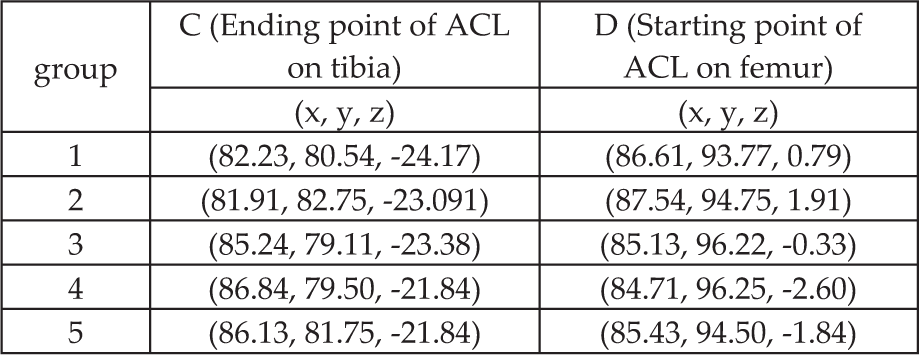
The range of the flexion angle of normal knee (θ ₁₂ ) during daily activities is 0°∼135°, but Blankevoort's research, within 90° the internal/external rotation of the tibia would not be restricted by the flexion angle of the femur, the ligament length changes are decided by the flexion angle. Because the calculation of the length of the ligaments is based on the assumption that the ACL is isometric during the knee's flexion, considering the disparity of the starting and ending points of ACL, five groups of data (Table 3) are used to analyse the sensitivity of the ligament length and femur rotation angle changes impacted by ACL positions. The changing curves of ligament lengths and internal/external angles with respect to flexion angles are depicted in Figure 6. The maximal deviation of PCL length is less than 0.28 mm, the LCL length is less than 0.83 mm, the MCL length is less than 0.12 mm and the degree of rotation angle is less than 3.16°.

Figure 6

Feature sizes and angles as ACL position changes, (a) degree of external/internal angle, (b) length of PCL, (c) length of LCL, (d) length of MCL

Table 3.

The starting and ending sites of the ACL

group	C (Ending point of ACL on tibia)	D (Starting point of ACL on femur)
	(x, y, z)	(x, y, z)
1	(82.23, 80.54, −24.17)	(86.61, 93.77, 0.79)
2	(81.91, 82.75, −23.091)	(87.54, 94.75, 1.91)
3	(85.24, 79.11, −23.38)	(85.13, 96.22, −0.33)
4	(86.84, 79.50, −21.84)	(84.71, 96.25, −2.60)
5	(86.13, 81.75, −21.84)	(85.43, 94.50, −1.84)

As shown in Figure 6, when the flexion angle changes from 0° to 90°, the length of LCL decreases monotonically indicating that the LCL is under maximum tension when the knee is completely extended, which is in agreement with anatomy results. Contrary to PCL, the tension on MCL/PCL first increases/decreases then decreases/increases which is in agreement with Blankevoort's results. When the flexion angle reaches 20° [10], the degree of rotation angle gradually increases along with the increase of the flexion angle, which is also in agreement with Akalan's results [11].

Moreover, in order to analyse the sensitivity of the tibia medial condyle contact point position, five contact points are chosen (Table 4). The result curves show that the tendency of the changing of ligament lengths remains the same and the maximal deviation of internal/external angle is less than 0.15°, the length of PCL is less than 0.05 mm, the length of LCL is less than 0.02 mm and the length of MCL is less than 0.01 mm. This result indicates that the impact of contact point position is insignificant.

Table 4.

Position of contact point on the medial condyle of the tibia

group	Point A: tibia medial condyle contact point
	x/mm	y/mm	z/mm
1	112.21	81.26	−29.56
2	112.85	84.03	−29.69
3	114.26	82.19	−29.71
4	110.74	82.88	−29.71
5	114.96	82.88	−29.94

The simulation results of the tibio-femoral contact force after ACL reconstruction is shown in Figure 7. As the flexion angle changes from 0#x00B0; to 90°, the articular contact force first decreases and then increases in all of the X-axis, Y-axis and Z-axis directions. The minimum contact force on X-axis is around 45°, Y-axis around 35° and Z-axis around 65°. Moreover, when different initial tensions are applied on the ACL, the contact force increases slightly as the initial tension increases, but the tendencies of the curves are almost the same. The impact of initial ACL tension on other tissues (such as articular cartilages and menisci) will be studied further in the future.

Figure 7

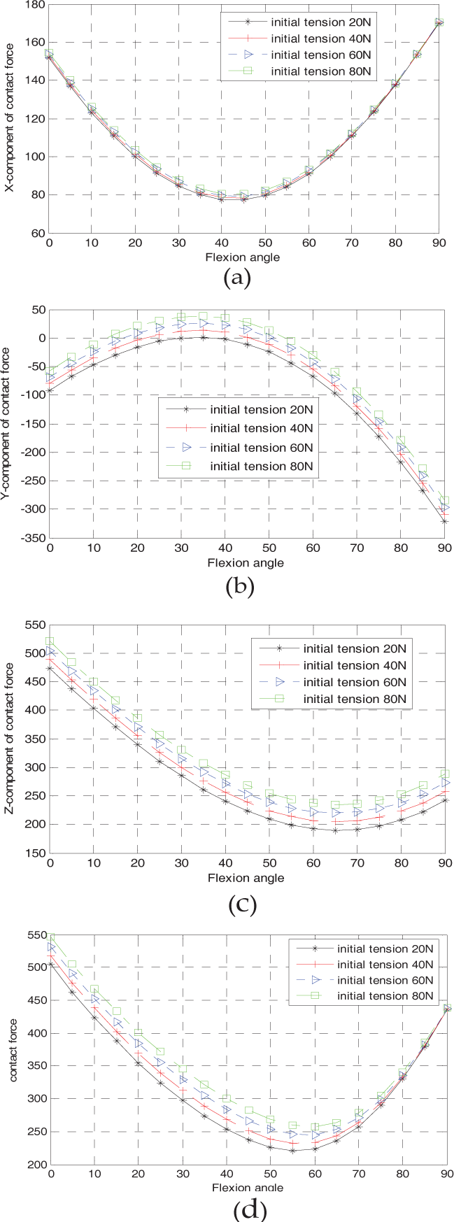
The contact force of tibio-femoral joint during knee flexion, (a) force of x-component, (b) force of y-component,(c) force of z-component, (d) magnitude of contact force

4. Conclusions

In this study a novel spatial mechanism was proposed to simulate the knee joint motion based on a three dimensional model of the human knee. The feature elements were extracted from the 3D model according to the anatomy and characteristic motion of the tibiofemoral joint, where the ACL fibres were assumed isometric and the other three ligaments were modelled as two links connected with a prismatic joint. The forward kinematics was solved using screw theory, the results show that the changing length of each ligament was in agreement with the early reference. The main strength of the proposed model is that it associates the knee's flexion motion with internal/external rotation of the tibia based on the isometricity of anterior cruciate ligament. This offers an efficient method to model and analyse the changes of ligament lengths and static kinematics after ligament reconstruction. The results obtained from the proposed model conform to that observed by Blankevoort et al. and they are also helpful in designing knee recovery and rehabilitation equipment.