Sage Journals: Discover world-class research

Abstract

This paper proposes a control strategy for a cable-suspended robot based on an optimal sliding mode approach confronted by external disturbances and parametric uncertainties. This control algorithm is based on the Lyapunov technique, which is not only able to provide the stability of the end-effector with an acceptable precision but also provides the optimal path in which the maximum load can be carried along. In addition, the optimization of the robot is performed based on an optimal sliding mode (SMC) approach. Tracking a predefined trajectory, path planning and the calculation of its relevant Dynamic Load Carrying Capacity (DLCC) is done based on the motors' torque and accuracy constraints. Optimal SMC, as a robust control algorithm, is used for controlling the stability of the system, while the Linear Quadratic Regulator (LQR) optimization tool is employed in order to optimize the controller gains. The main contribution of the paper is in calculating the DLCC of the cable robot. Finally, the efficiency of the proposed method is illustrated by performing some simulation studies on the ICaSbot (IUST Cable-suspended Robot), which supports six DOFs using six actuating cables, and experimental results confirm the validity of the authors' claim.

Keywords

Suspended Robot Sliding Mode Control (SMC)Dynamic Load Carrying Capacity (DLCC)Linear Quadratic Regulator (LQR)

1. Introduction

Cable transporter systems are widely used in industry, such as in high-rise elevators, cranes, conveyer belts and tethered satellite systems, etc. A cable-suspended robot typically consists of a moving platform that is connected to a fixed base by several cables. A cable-suspended robot can precisely manoeuvre large loads and is resistant to environmental perturbations. The main advantages of cable-suspended robots over conventional robots are: 1) a larger workspace for the same overall dimension of the robot, and 2) light weight cables resulting in a very safe and transportable system. These robots often present very high payload-to-weight ratios. In practice, there are some optimal control problems and so the optimization of this critical parameter can be a valuable objective in minimizing any extra power and energy consumption. The spatial sample is a particular type of cable robot with six cables. Optimizing the payload of the robot – as the most important parameter of this kind of robot – can be useful in the study of different applications. Alp and Agrawal [1] addressed the kinematic and dynamic models, workspace, trajectory planning and feedback controllers for parallel cable manipulators and performed simulation and experiments on a 6-DOF cable-suspended robot. Cables have a unique property since they cannot provide compression force on an end-effector. This constraint leads to performance deterioration and even instability if it is not properly accounted for in the design procedure. Several techniques have been suggested to guarantee positive tension in the cables while the end-effector is moving [1–2]. The static workspace is defined as the set of positions wherein any operational force can be exerted on the end-effector while all of the cables are in positive tension [3]. There have been a number of researchers who have applied various controllers and dynamic modelling for cable-actuated robots, such as the feedback linearization control method. There are two kinds of optimal controller: open-loop and closed-loop. Some related recent work on the open-loop optimal control of cable robots includes the following. Wang performs an open-loop optimal control of cable robots in order to minimize the cables' tension. The MAP method (Method of approximate programming) is utilized in order to optimize a parallel system by [4]; moreover, Korayem et al. used the Hamilton-Jacobi-Bellman (HJB) method to plan the optimal path for the same cable robot based on the DLCC objective function [5]. In an open-loop controller, any kind of disturbance or parametric uncertainty ruins the desired results. In decreasing the number of these failures, researchers have suggested using a closed-loop controller. Closed-loop studies have also been accomplished based on the variation of objective functions. In [6], there is presented a homogeneous controller for tracking the trajectories of robot manipulators. The allowable workspace is maximized in [7] using the closed-loop method. On the other hand, path planning for soccer robots using PSO (Particle Swarm Optimization) has been done by Wang [8]. Furthermore, the output regulation problem for a servomechanism with nonlinear backlash is proposed as a case study in [9] and an observer is designed in order to eliminate the difficulty of working with various variables for the design of type-1 fuzzy controllers. [10] describes the use of a genetic algorithm (GA) for the problem of offline point-to-point autonomous mobile robot path planning. Also, path planning for robots with motion uncertainty and imperfect state information is performed using a LQG (Linear Quadratic Gaussian) approach [11]. In [12], a model for a flexible cable transporter system with arbitrarily varying cable lengths is presented. It is shown that the SDRE technique (State dependent Riccati Equation) is applicable for flexible cable systems with varying lengths, while guaranteeing the performance of the closed-loop system. Furthermore, an algorithm for the calculation of the DLCC for a rigid cable robot which is under a closed-loop controller has been presented [13]. Moreover, designing a sliding mode controller as a stabilizing controller for a given uncertain system has been employed in [14]. The range of the system states in terms of set points is found and the states in the inequalities of the input are substituted so that the constraints are satisfied. In contrast to the general control laws, sliding mode control is more robust and easier to implement. The closed-loop optimal control of cable robots for the calculation of the maximum dynamic load carrying capacity of cable robots is done by using a feedback linearization controller with a LQR optimization method [15]. Carrying the payloads is one of the important applications of cable-suspended robots in the aerospace industry. Both military and commercial operators exploit this capability of helicopters to rapidly move heavy loads to locations where the use of ground-based equipment for transport is not possible. The transport of externally-suspended loads is an important mission for a helicopter. In particular, helicopters are actively used for ship replenishment and hoist operations from seagoing cargo vessels, especially in adverse weather [16].

Tracking the optimal path with admissible error in a closed-loop manner while the highest load is carried along is ignored in the literature. This method in planning the path considerably increases the accuracy of final point compared to open-loop approaches and decreases its DLCC. Therefore, in this paper, a combination of SMC with LQR is applied for the accurate optimal path planning of a cable system subject to its DLCC. The sliding mode approach is employed for stabilization and path planning between two specified points. Moreover, the DLCC of a cable robot is evaluated in a closed-loop manner using the SMC method. A sliding mode is a nonlinear feedback control with a variable structure with respect to the system states. The main advantage of a sliding mode control is that the system is insensitive to extraneous disturbance and internal parameter variations while the trajectories are on the switching surface. There are two important factors that should be considered while calculating the DLCC of a robot with this method, namely the maximum torques that can be applied by the motors and the maximum acceptable bounds of errors that the end-effector is permitted to move within. The required constraints can be easily satisfied with the aid of the proposed iterative algorithm, which is based on a SMC approach. In addition, the linearization of the equations makes it possible to use a LQR method in order to optimize the system for a defined objective function. This paper illustrates a new, combined algorithm that uses both sliding mode and LQR. Indeed, sliding mode control gains are optimized using a LQR method. The nonlinear state space of SMC is first linearized with the aid of a piecewise linearization method. Afterwards, LQR is employed to optimize the gains of each part separately. The sliding mode control algorithm is based on the Lyapunov technique, which confirms its strategy. Moreover, a stable pole placement with a satisfactory phase and gain margin is offered by a LQR optimizer. Since the payload of the end-effector is supposed as an important uncertainty, the closed-loop optimization method should be robust. A survey of recent developments shows that other methods are not robust or adequate. Therefore, the superiority of the presented closed-loop optimization (optimal sliding mode) over previous methods lies in its better robustness, which can provide higher DLCC capability.

The paper is organized as follows: first, the dynamic equations of the spatial cable robot are derived. Next, a Sliding Mode Control is presented as a powerful method for uncertain nonlinear systems under the condition of the absence of disturbance and in the presence of disturbance for a predefined trajectory. Afterwards, path planning is done based on the motors' torque constraint and accuracy constraint, while the control gains are optimized using the LQR method after linearization. Finally, an algorithm is proposed to compute the maximum allowable load by considering the limiting factors. In the last section, the efficiency of the proposed algorithm is verified by comparing the simulations with experimental tests conducted on the ICaSbot.

2. Dynamical Modelling

For the spatial case, assume a triangular-shaped end-effector, as shown in Figure 1, which is suspended by six cables and has 6 degrees of freedom as X = {x, y, z, ψ, Θ, φ}. The coordinate system of translational movement, which is established on the fixed platform, is global while the coordinate system of the rotational movement, which is established on the end-effector, is local. It is provable that the dynamical equation can be shown as [1]:

D (X) \ddot{X} + C (X, \dot{X}) \dot{X} + g (X) = - S_{J}^{T} (q (X)) T;

(1)

Figure 1.

Spatial model of the cable robot [1]

where:

\begin{array}{l} D = [\begin{matrix} m I_{3} & 0 \\ 0 & P^{T} I P \end{matrix}]; C = [\begin{matrix} 0_{3} \\ P^{T} {I \dot{P} \dot{ο} + (P \dot{ο}) \times I (P ο)} \end{matrix}]; g = [\begin{matrix} 0 \\ 0 \\ - m g \\ 0_{3} \end{matrix}] \\ S_{J} = {[\frac{\partial q_{i}}{\partial x_{j}}]}_{i \times j}; P = [\begin{matrix} 1 & 0 & - \sin θ \\ 0 & \cos ψ & \sin ψ \cos Θ \\ 0 & - \sin ψ & \cos ψ \cos Θ \end{matrix}]; \dot{ο} = [\begin{matrix} \dot{Ψ} \\ \dot{Θ} \\ \dot{φ} \end{matrix}] \end{array}

where D(x) is the inertia matrix for the system, C(X, Ẋ) is the matrix of the Coriolis and centripetal terms, g(x) is the vector of the gravity terms, T is the vector of the cables' tension, S_J is the conventional parallel manipulator Jacobian, X is the vector of the DOFs of the system, m is the mass of the end-effector, I is the moment of inertia of the end-effector and q is the length of the cables. In addition, the dynamics of the motor are as follows:

\begin{array}{l} T = 1 / r (τ - J (d / d T (\partial β / \partial X) \dot{X} + \ddot{X} (\partial β / \partial X)) \\ - C (\partial β / \partial X) \dot{X}) \end{array}

(2)

where J is the matrix of the rotary inertia of the motors, c is the viscous friction matrix of the motors, $\dot{β}$ is the vector of the angular velocity of the motors and τ is the vector of the motors' torque. By coupling these two dynamics, we have:

\begin{array}{l} T = 1 / r (τ - J (d / d T (\partial β / \partial X) \dot{X} + \ddot{X} (\partial β / \partial X)) - C (\partial β / \partial X) \dot{X}) \\ D (X) \ddot{X} + C (X, \dot{X}) \dot{X} + g (X) = - S_{J}^{T} (q (X)) T \end{array}

(3)

3. Control Scheme

3.1 Sliding Mode Control

The following equation is considered:

X^{n - 1} = f (X) + b (X) u

(4)

For the indicated cable robot, the order of the system is (n=2), following sliding surface which is considered:

s = {(\frac{d}{d t} + λ)}^{n - 1} e

(5)

where:

e = X - X_{d}

(6)

s is called the ‘sliding surface’. In particular, the Lyapunov sliding condition forces the system states to reach a hyperplane and keeps them from sliding on this hyperplane. Essentially, a SMC design is composed of two phases: hyperplane design and controller design. However, in this paper, a method proposed by Slotine is used [17]. Accordingly, the sliding surface is defined as:

s = (\frac{d}{d t} + λ) (X - X_{d}) = (\dot{X} - {\dot{X}}_{d}) + λ (X - X_{d})

(7)

To determine the control law, the derivative of the sliding surface must be determined:

\dot{s} = (\ddot{X} - {\ddot{X}}_{d}) + λ (\dot{X} - {\dot{X}}_{d})

(8)

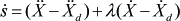
since the sliding condition is defined by:

\dot{s} \leq - k . S i n g (s)

(9)

As such, Eq. 9 – in order to satisfy the sliding condition – must be written as:

(\ddot{X} - {\ddot{X}}_{d}) + λ (\dot{X} - {\dot{X}}_{d}) = - k . S i n g (s)

(10)

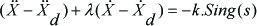
In the sliding mode control, λ,k are the constant gains of the control system. By substituting Ẍ from Eq. 10 in Eq. 1, it can be written as below:

\begin{array}{l} D (X) {{\ddot{X}}_{d} - λ (\dot{X} - {\dot{X}}_{d}) - k . S i n g (s)} \\ + C (X, \dot{X}) \dot{X} + g (X) = - S_{J}^{T} (q (X)) T \end{array}

(11)

Combining Eqs. 2 and 11, they can be expressed based on motor torque:

\begin{array}{l} τ = S_{J}^{- T} {r D [k s i g n (s)] + r D λ (\dot{X} - {\dot{X}}_{d}) - r D {\ddot{X}}_{d} - r C \dot{X} - r g} \\ + J \ddot{β} + c \dot{β} \end{array}

(12)

Then, the optimal path can be calculated by the following formula:

\begin{array}{l} X = \iint {D^{- 1} (- S_{J}^{T} [1 / r (S_{J}^{- T} {W})] - g - C \dot{X})} d t \\ W = {r D [k s i g n (s)] + r D λ (\dot{X} - {\dot{X}}_{d}) - r D {\ddot{X}}_{d} - r C \dot{X} - r g} \end{array}

(13)

Not only is the employed strategy robust, but so too is the stability of the employed controlling strategy guaranteed based on Lyapunov. In addition, the optimizer tool of LQR provides a stable pole placement with an acceptable phase and gain margin.

3.2 Optimal Control Implementation

In order to find the DLCC, two main constraints – including the required motor torque and tracking error – are considered, which are supposed to be minimized using the LQR method for achieving the highest load capacity. Therefore, Eq. 10 is linearized and estimated to three linear formulations using piecewise linearization. Now, it is possible to use LQR for the optimization of the closed-loop control gains. The whole control procedure is demonstrated in Figure 2. The motors' torque and end-effector errors are the terms of the objective function to be minimized for the movement of the end-effector, and so the cost function can be defined as Eq. 14. In this cost function, time is not considered as the terms of the objective function since it is not involved in the DLCC constraints. When both motors' torques – which are called, u(X, t) – and tracking error constraints – which are called e(X, t) – saturate simultaneously, the optimal path is achieved:

J (x, t) = \int_{t}^{\infty} (e_{l} {(X, t)}^{T} Q e_{l} (X, t) + u {(X, t)}^{T} R u (X, t)) d τ

(14)

Figure 2.

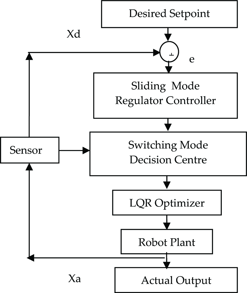
Control procedure of the robot based on the optimal sliding mode

where Q is the gain matrix of accuracy, R is the gain matrix of the control input and e_l(X, t) contains e(X, t), e(X, t). Both of them are a symmetric positive definite matrix. Solving this cost function for a closed-loop state space using the Hamilton-Jacobi-Bellman equation results in the following Riccati equation, where the stability is assured using the Lyaponov equation [18]:

S A + A^{T} S + Q - S B R^{- 1} B^{T} S = 0

(15)

Figure 3.

Piecewise linearization of the SMC methodology

where Q is the gain matrix of the accuracy, R is the gain matrix of the control input, A and B are state space matrixes of closed-loop system. Solving the Riccati equation for S results in the following optimal control input:

\begin{array}{l} u_{F}^{*} = K_{F}^{*} [e (X, t); \dot{e} (X, t)] = k_{p} e + k_{d} \dot{e} \\ K_{F}^{*} = - R^{- 1} B^{T} S \end{array}

(16)

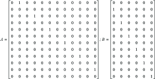
k_p is the gain of position error and k_d is the gain of the velocity error. The state equations with the LQR method can be rewritten as follows:

\begin{array}{l} \dot{e} (t) = A e (t) + B u (t) \\ {\begin{cases} {\dot{e}}_{i} = e_{i + 1}; i = 1, 3, 5, …, 11 \\ {\dot{e}}_{i + 1} = {- R^{- 1} B^{T} S [e (X, t); \dot{e} (X, t)]}_{j}; j = 1, 2, 3, …, 6 \end{cases} \end{array}

(17)

Here, matrixes A and B are defined as below:

A = [\begin{matrix} 0 & 1 & 0 & 0 & 0 & 0 & 0 & 0 & 0 & 0 & 0 & 0 \\ 0 & 0 & 0 & 0 & 0 & 0 & 0 & 0 & 0 & 0 & 0 & 0 \\ 0 & 0 & 0 & 1 & 0 & 0 & 0 & 0 & 0 & 0 & 0 & 0 \\ 0 & 0 & 0 & 0 & 0 & 0 & 0 & 0 & 0 & 0 & 0 & 0 \\ 0 & 0 & 0 & 0 & 0 & 1 & 0 & 0 & 0 & 0 & 0 & 0 \\ 0 & 0 & 0 & 0 & 0 & 0 & 0 & 0 & 0 & 0 & 0 & 0 \\ 0 & 0 & 0 & 0 & 0 & 0 & 0 & 1 & 0 & 0 & 0 & 0 \\ 0 & 0 & 0 & 0 & 0 & 0 & 0 & 0 & 0 & 0 & 0 & 0 \\ 0 & 0 & 0 & 0 & 0 & 0 & 0 & 0 & 0 & 1 & 0 & 0 \\ 0 & 0 & 0 & 0 & 0 & 0 & 0 & 0 & 0 & 0 & 0 & 0 \\ 0 & 0 & 0 & 0 & 0 & 0 & 0 & 0 & 0 & 0 & 0 & 1 \\ 0 & 0 & 0 & 0 & 0 & 0 & 0 & 0 & 0 & 0 & 0 & 0 \end{matrix}]; B = [\begin{matrix} 0 & 0 & 0 & 0 & 0 & 0 \\ 1 & 0 & 0 & 0 & 0 & 0 \\ 0 & 0 & 0 & 0 & 0 & 0 \\ 0 & 1 & 0 & 0 & 0 & 0 \\ 0 & 0 & 0 & 0 & 0 & 0 \\ 0 & 0 & 1 & 0 & 0 & 0 \\ 0 & 0 & 0 & 0 & 0 & 0 \\ 0 & 0 & 0 & 1 & 0 & 0 \\ 0 & 0 & 0 & 0 & 0 & 0 \\ 0 & 0 & 0 & 0 & 1 & 0 \\ 0 & 0 & 0 & 0 & 0 & 0 \\ 0 & 0 & 0 & 0 & 0 & 1 \end{matrix}]

The state equations with the SMC method, according to Eq. 10, can be rewritten as follows:

{\begin{cases} {\dot{e}}_{i} = e_{i + 1}; i = 1, 3, 5, …, 11 \\ {\dot{e}}_{i + 1} = {- k S i g n (s) - λ \dot{e}}_{j}; j = 1, 2, 3, …, 6 \end{cases}

(18)

Here, and in order to use LQR as an optimizer tool for linear systems, a piecewise linearization method is used for Eq. 18 to divide the Sign(s) into three linear parts which can be optimized separately using LQR. This linearization results in the following controlling inputs for each area:

{\begin{cases} u_{S}^{*} = k + λ (\dot{e} (X, t)) = K_{S}^{*} [e; \dot{e}]; s > 2.5 \\ u_{S}^{*} = - k + λ (\dot{e} (X, t)) = K_{S}^{*} [e; \dot{e}]; s < - 2.5 \\ u_{S}^{*} = 0.1 k s + λ (\dot{e} (X, t)) = K_{S}^{*} [e; \dot{e}]; - 2.5 < s < 2.5 \end{cases}

(19)

This control input is then considered to be equal with the optimized one of Eq. 16. In fact, the state space equations of LQR and SMC are compared in Eqs. 17 and 18 and then the optimal k, λ gains are calculated as follows:

K_{F}^{*} = K_{S}^{*} \to {\begin{cases} {\begin{cases} k = k_{p} e \\ λ = k_{d} \end{cases} \to s > 2.5 \\ {\begin{cases} k = - k_{p} e \\ λ = k_{d} \end{cases} \to s < - 2.5 \\ {\begin{cases} 0.1 k λ = k_{p} \\ 0.1 k + λ = k_{d} \end{cases} \to - 2, 5 < s < 2.5 \end{cases}

(20)

4. Determining the Maximum Load Carrying Capacity

The dynamics of the cable robot can be used to extend its payload capability while taking into account torque and tension as realistic constraints. By considering the actuator torque and accuracy constraints and adopting a logical computing method, the maximum load-carrying capacity of a cable robot for a predefined trajectory can be computed. The actuator torque constraint is formulated based on the typical torque-speed characteristics of DC motors [13]:

τ_{u} = k_{1} - k_{2} \dot{q}; τ_{l} = - k_{1} - k_{2} \dot{q}

(21)

where τ_u and τ_l are the upper bound and the lower bound of actuator constraint respectively. The coefficients k_i are defined as:

k_{1} = T_{s}; k_{2} = \frac{T_{s}}{w_{n l}}

(22)

where T_s is the stall torque and w_nl is the maximum no-load speed of the motor. The algorithm used for finding the DLCC in the closed-loop case is shown in Figure 4. The actuator torque at each point is computed with respect to its bounds and the accuracy of the end-effector tracking is determined. Using this method, we can find DLCC at each time and so it will be identified for the whole of the path.

Figure 4.

Flowchart of the computing dynamic load carrying capacity

The maximum DLCC is estimated using the mentioned iterative process in which a pure analytic process is done in each repetitious trend (SMC+LQR). As such, the maximum DLCC is evaluated using an analytic method, which is secure from non-conversancy or local optimization syndrome.

5. Simulation Results for a Predefined trajectory

5.1 Simulation of Control Procedure

To investigate the proposed controller, some simulation studies are presented for a spatial robot.

In these studies, a circular trajectory is assumed whereby the end-effector with the controller follows the path perfectly. The simulation results are shown in the Figures. The parameters used in the simulation are given in Tables 1 and 2. The motor input-output path, torque, cable tension and error profile are shown in Figures 5 and 6. It is observable that all of the cable tensions are positives, as it was expected. It can be seen than an excellent compatibility exists between the input and output with the aid of the proposed SMC method. Practical robotic systems have inherent system perturbations, such as parametric uncertainties and external disturbances – e.g., static friction, noise in control signals, etc. In this paper, the behaviour of the cable robot in the presence of external disturbances is also considered. Let us denote the disturbances by d = 0.5Sin(5t), which is applied to the control input according to Eq. 12. The real dynamic equation of the cable robot with the disturbance term is represented as follows:

\begin{array}{l} τ = S_{J}^{- T} {r D [k s i g n (s)] + r D λ (\dot{X} - {\dot{X}}_{d}) - r D {\ddot{X}}_{d} - r C \dot{X} - r g} \\ + J \ddot{β} + c \dot{β} + d \end{array}

(23)

Table 1.

Reference input for a spatial simulation

\begin{array}{l} t < & = 4, \\ x = 0.05 * cos (4 * pi * (t^2) / 64), \\ y = 0.05 * sin (4 * pi * (t^2) / 64), \end{array}

\begin{array}{l} t > & 4 \\ x = 0.05 * cos (4 * pi * ((- t + 8)^2) / 64) \\ y = - 0.05 * sin (4 * pi * ((- t + 8)^2) / 64) \end{array}

\begin{array}{l} z = 0.45; ψ = 0 \\ Θ = 0; φ = 0 \end{array}

Table 2.

Characteristics of the spatial system

Name	Symbol	Value	Unit
Momentum of the inertia of the end-effector	I	Ixx = Iyy = 1847779.1510⁶ Izz=2Ixx	kgm ²
Control coefficient	λ	diag[20]
Control gain	K	diag[200]
Radius of the motor	r	diag[0.015]	m
Momentum of the inertia of the pulley	J	diag[3309.21*10^(–9)]	kg.m²

Figure 5.

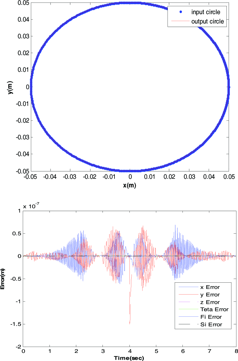
Input-output path and error of the spatial simulation in the absence of disturbance

Figure 6.

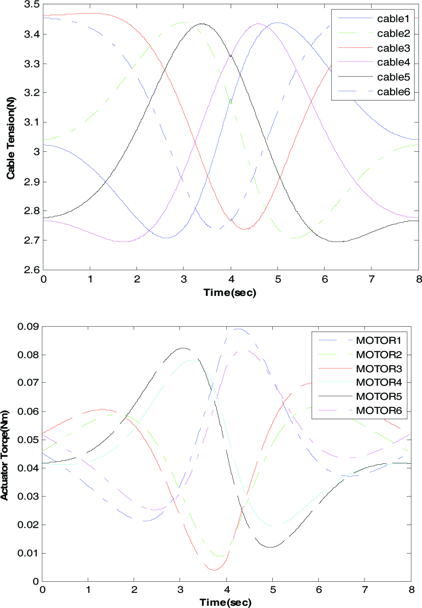
Torques and tensions profiles of the spatial simulation in the absence of disturbance

The dynamic response of the system in the presence of disturbance is shown in Figures 7 and 8:

Figure 7.

Input-output path of the spatial simulation in the presence of disturbances

Figure 8.

Torques, tensions and error profiles of the spatial simulation in the presence of disturbances

It can be seen that the destructive external disturbance is successfully filtered with the aid of the proposed SMC controller since the fluctuations are neutralized by automatically the switching of the actuators' torque, which eventually provides a smooth tracking with an acceptable error. However, the most sensitive DOF that shows the highest error is related to z, which is engaged with gravity effects and, again, is controlled properly with the aid of the proposed SMC. Now, a comparison between the employed controlling strategy in this paper and the feedback linearization approach is performed in Figure 9 in order to control the end-effector on a desirable path in a closed-loop manner [13] in the presence of disturbance, such as d = 0.5sin(50t). This simulation is done on a cable robot with 2-DOFs using three actuating cables. A circular trajectory of the cables is assumed.

Figure 9.

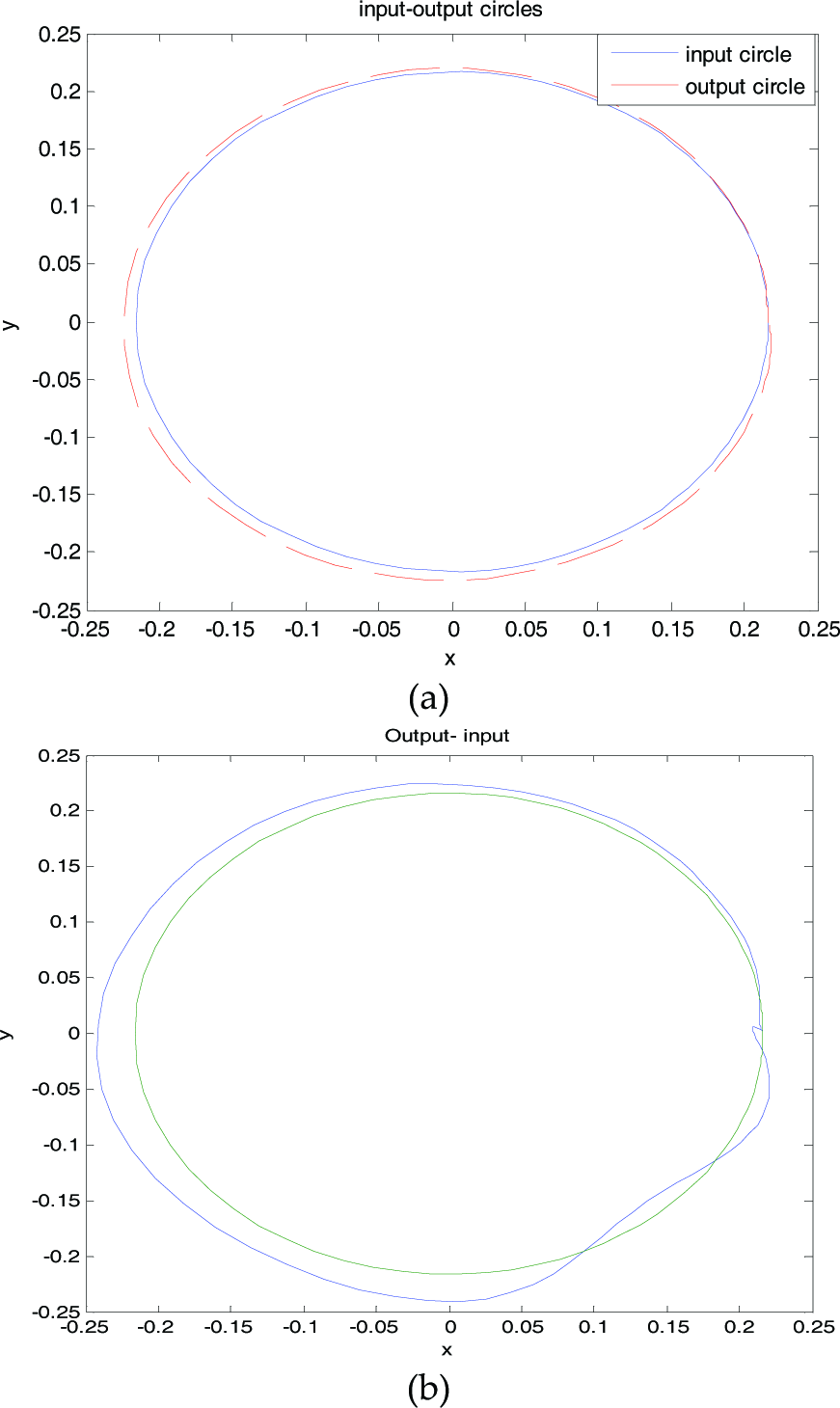
Input-output path in the absence of disturbance based on the SMC method (a) and based on the LQR method (b)

It can be seen that feedback linearization suffers from instability while stability is guaranteed in the proposed optimal SMC. As was shown, the optimal SMC method has improved the trajectory of the predefined path in comparison to the optimal feedback linearization method.

5.2 Simulation of the DLCC Algorithm

Based on the mentioned algorithm of the maximum payload, the calculation of DLCC according to the upper and lower limits of the torques and accuracy is performed. The saturation of motors' torque is presented in Figure 10 and, as can be seen, the first and fifth motors are saturated at the middle of the simulation.

To achieve the maximum payload, the optimizer tool should provide the gains in manner such that the torque and error saturate simultaneously. This expectation can be seen to be satisfied here. As was shown in Figure 11, the error constraint is saturated for the system. By applying the proposed algorithm for closed-loop plant when the motors' torque and tracking error constraints saturate simultaneously, the maximum allowable load is computed about m_p =4.7kg.

Figure 10.

Saturation profile of the motor' torques in the spatial simulation

Figure 11.

Error profiles of the spatial simulation

6. Simulation Results for Path Planning

6.1 Simulation of the Control Procedure

In this section, a simulation is performed for moving between point (0.05, 0, and 0.45) and point (0, 0, and 0.1). The applied boundary conditions in the simulation are displayed in Table 3 and other specifications are listed in Table 4.

Table 3.

Properties of the simulated spatial robot

Name	Symbol	Value	Unit
Half of the base and triangle end effector	a,b	0.59,0.085	m
Error gain matrix	Q	diag[1];z = 10,
Input gain matrix	R	diag[1];z = 0.1

Table 4.

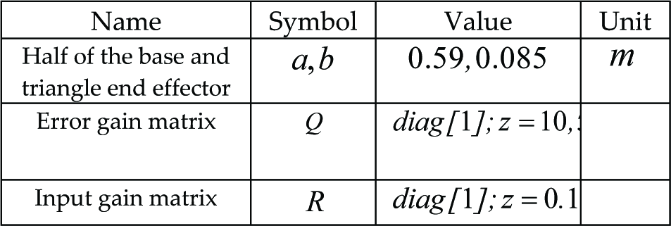
Simulated motor characteristics of the spatial cable robot

Parameter	Symbol	Value	Unit
Added mass	m_l	4	kg
Motor's Max. no load speed	ω_n	286.47	Rad/s
Motor stall torque	τ_s	0.75	N.m

The objective of the optimization is torque and error. Time is not considered as the cost function of the optimization process and so LQR with infinite time is used. However, the time of the end-effector convergence to the set point is controllable by increasing or decreasing the accuracy matrix of LQR (Q). The simulations show that the convergence occurred in a logical finite time (about 10 seconds). The payload of the end-effector is increased as the parametric uncertainty, from 1kg up to 3kg. The simulations of the optimal path and errors with two various error gains are shown in Figures 12 and 13.

Figure 12.

Optimal path planning between two points with different controller gains

Figure 13.

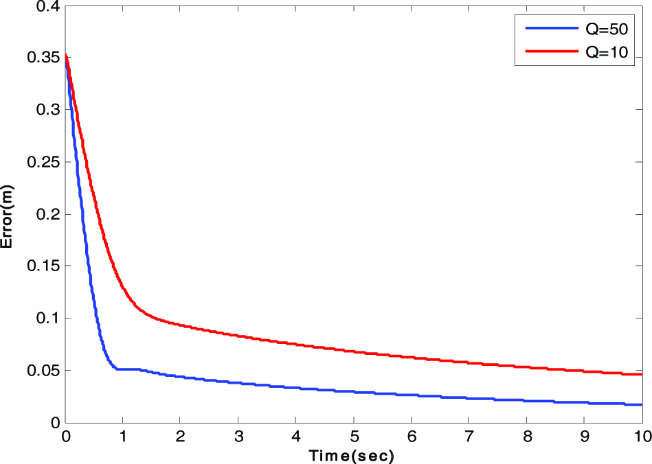
Error profile between two points with different controller gains

As was shown, the accuracy of regulation process is increased because of enhancement of the controller gains from Q=10 to Q=50. The error profiles illustrate that the controller with higher gains has an error equal to 0.01m while the controller with lower gains has an error of 0.04m. The torque of motors 1, 5 and 6 is compared for two different controller gains as a sample in Figure 14.

Figure 14.

Torque profile between two points with different controller gains

First of all, it can be seen that in the first moments, and because of the greatest error, the amount of torque is maximum so as to compensate for this error. Afterwards, the torque reduces logarithmically. Again, it is obvious that controller with the higher error gains applies further torque for the enhancement of final point accuracy and so the torque of the controller with Q=50 is higher than the controller with Q=10. Accordingly, the coefficients of SMC for Q=50 are calculated as a sample and are shown in Figure 15.

Figure 15.

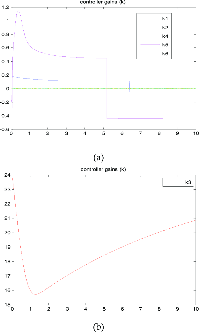
The error gains of the x,y,ψ,Θ,φ directions (a) and the error gain of the z direction (b)

It can be seen that, as a consequence of the gravity on the load, the error of the end-effector in the z direction is of an upper order compared to the other DOFs; as such, and based on this detail, the error gain of the z direction has to be selected as significantly bigger than the other DOFs (Figure 15). Also, it is proven here that the optimal gain of SMC needs to change during the time so as to produce the optimal path with the least energy.

6.2 Simulation of the DLCC Algorithm

It should be mentioned that, in each of the simulation cases, increasing the load in the iteration loop is performed until the first motor saturates simultaneously with the accuracy constraint. According to the precision constraint, the payload of the robot can be increased as long as the end-effector error does violate the permissible error bound. This procedure is repeated for heavier payloads until the first error saturation occurs. The DLCC of robot is the load, for which the torque and error remain within the permissible error bound. The simultaneous optimization of the torque and error is the main method in order to maximize the DLCC of the robot. The same algorithm results in about a 4kg load capacity, which causes the first saturation at motors 2, 4 and 6, as is shown in Figure 16, and the torques of other motors are the same and are shown in Figure 17.

Figure 16.

Saturation profile of the motor torques of the spatial simulation for motors 1, 3 and 5

Figure 17.

Saturation profile of the motor torques of the spatial simulation for motors 2, 4 and 6

As was mentioned above, in the first moments, the torque is at the highest value so as to compensate for the error which is at its maximum during the initial moments. Afterwards, the torque decreases logarithmically as a result of LQR usage. However, for the simulated boundaries, the movement is upward and so the opposite happens; consequently, motor saturation occurs during the final moments of the simulation. Moreover, it can be seen that error constraint is saturated for the closed-loop system for a 4kg payload while the motors' torque did not violate the allowable bound (Figure 18).

Figure 18.

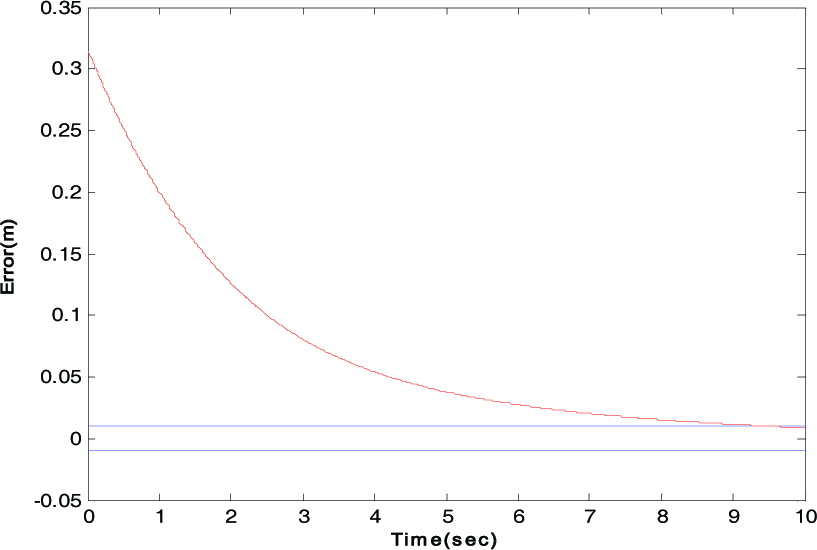
Error saturation profile

It can be seen that using the optimal SMC as a closed-loop controller considerably increases the accuracy of the final point compared to open-loop approaches (Figure 19). The red line is the optimal closed-loop approach, which has the minimum error at the final point with the adjustment of the coefficient of LQR.

Figure 19.

Planning of the optimal path

The SMC controller gains after the optimizations are shown in Figure 20.

λ = [- 10.9545 - 22.8035 - 71.8842 - 10.9545 - 10.9545 - 10.9545]

(24)

Figure 20.

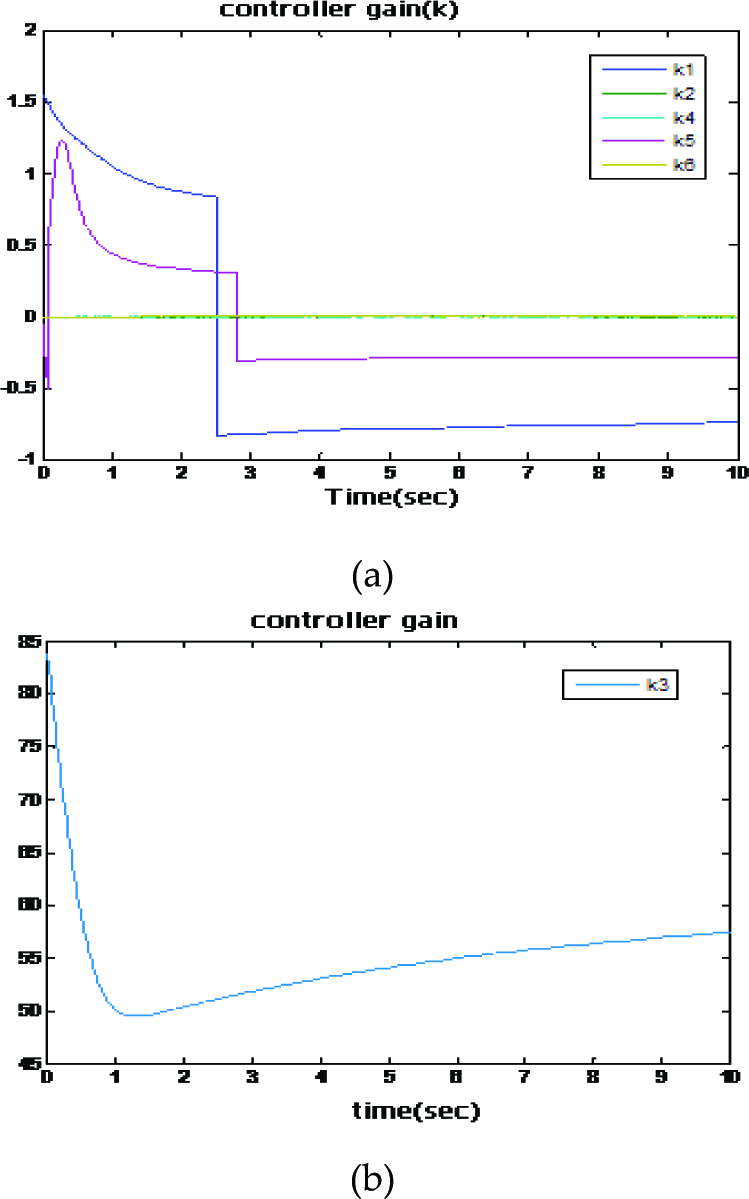
The error gains in the x,y,ψ,Θ,φ directions (a) and the error gain in the z direction (b)

As was mentioned in the previous section with regard to the spatial cable robot, because of the gravity effect on the load the error gain in the z direction – which is called k3 – is significantly bigger than the other error gains. Furthermore, the gains are time-dependent. By applying the proposed algorithm for a closed-loop plant, the maximum allowable load computed is m_p = 4kg where the motors are saturated.

7. Experimental Results for Path Planning

In this step, the simulation results should be verified by experiment. To provide an example, a point-to-point test is performed on the spatial cable-suspended robot, which is designed and manufactured in IUST, supporting 6-DOFs (Figure 21).

Figure 21.

Scheme of the designed IUST cable robot

The geometrical properties of the cable-suspended robot in IUST are listed in Table 5.

Table 5.

Features of the designed IUST cable robot

Body
Height	120cm
Side length of the base triangle	100–200cm
Weight	350kg
End-effector
Side length of the base triangle	17cm
Thickness	8cm
Weight	1,100g

Generally, the overall scheme of the optimal control of the ICaSbot in a closed-loop manner is depicted in the following flowchart. As it can be seen from Figure 22 the cable robot in the experimental test has been controlled in a closed-loop manner. The optimal path, which is gained by the SMC method, is used as the desired path in the experiment test. The optimal path between the following points is supposed to be extracted experimentally with the aid of the ICaSbot cable robot.

Figure 22.

Controlling strategy of the cable robot of ICaSbot for optimal regulation

The test is performed by moving between point (0.05, 0.05, 1) and point (-0.05, 0, 0.8). Some of the comparison profiles between the simulation and experiment results are shown. For example, the DOFs of the system and the velocity of some motors are plotted in Figures 23 and 24.

Figure 23.

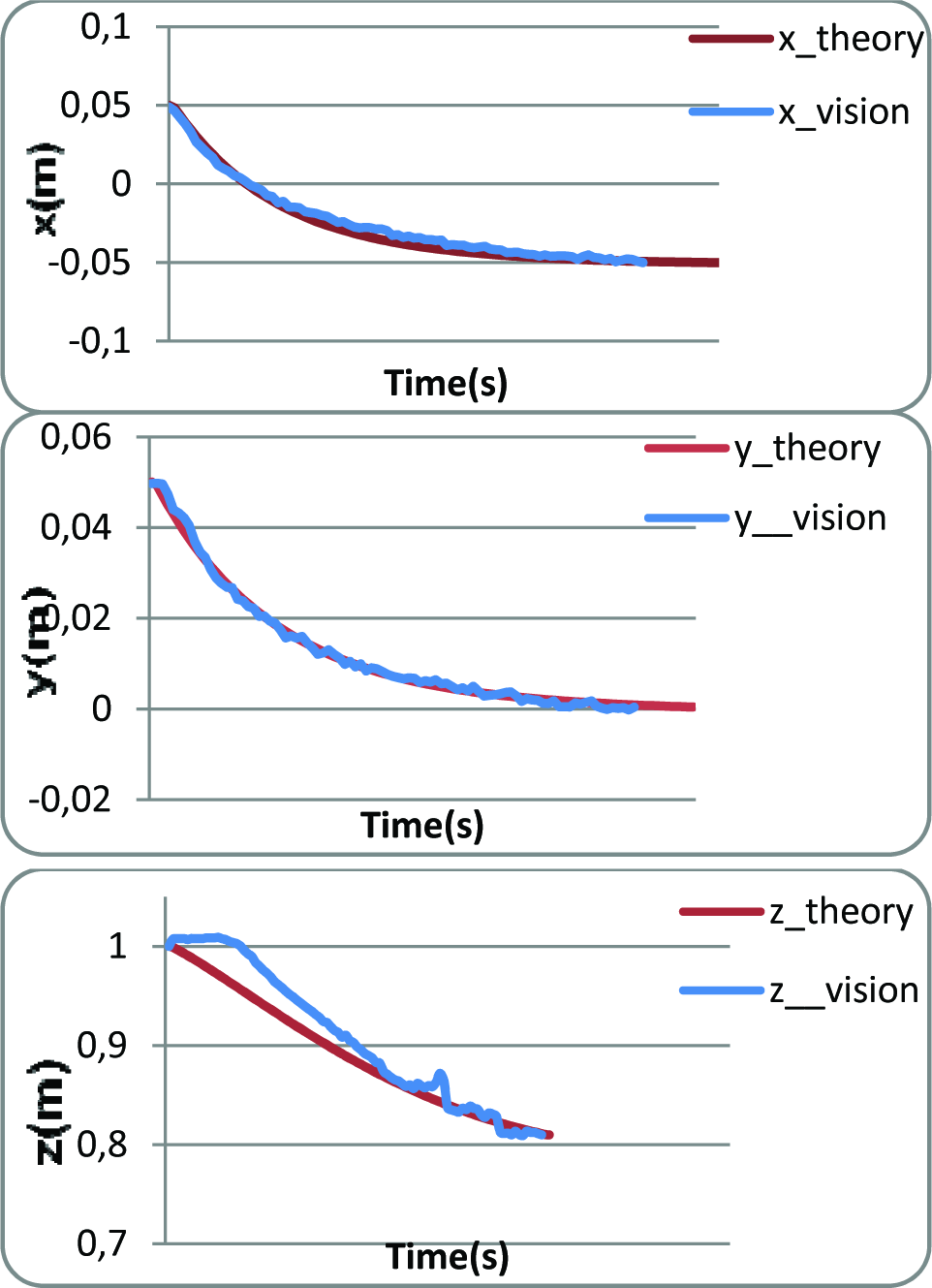
DOFs of the system in comparison with the experimental results

Figure 24.

Angular velocity of the motors in comparison with the experimental results

In point-to-point control, the profiles decrease logarithmically during the process. There are several reasons for the oscillatory behaviour of the experimental results, including motor clearance, cable vibration, the existence of the motor gearbox and the low accuracy of the sensors and encoders. The reason for the higher value of the motor speed for the simulation profiles during the initial moments of movement compared with the experimental results is due to the high inertia of the motor in reality. Moreover, since the most destructive effect is a result of gravity, the compatibility of the simulation and experiment is better for x,y rather than for z. These differences will be compensated for afterwards thanks to designed controller. According to these results, it can be seen that the experimental results are highly compatible with the simulation results and, thus, path planning can be easily performed with the aid of the proposed closed-loop controller based on an optimal SMC approach. The simulations illustrate the efficiency of the proposed method and the laboratory-based experimental test on a 6-DOF cable-suspended robot confirms them. Therefore, in this paper, SMC – as a robust control algorithm – is used. The advantage of the proposed algorithm lies in the calculation of the DLCC of the cable robot using a closed-loop computational technique based on the SMC algorithm. The controlling gains of the SMC are chosen in a way such that no considerable chattering occurs during the process of path planning. The simulation results demonstrate this claim since the path planning is done with a smooth parabolic decrease. However, the observed vibrations of the experimental results are due to the structural uncertainties of the manufactured ICaSbot (including those of the joint flexibilities, cable elasticity and structural frictions) and the low resolution of the employed sensors.

8. Conclusions and Discussion

This paper addressed the issue of the optimal control of a 6-DOF spatial cable robot of IUST. An optimal sliding mode control was implemented for it as a stabilizing controller insofar as it is faced with external disturbances and parametric uncertainties for a predefined trajectory. In addition, a new closed-loop optimal control method between two points was presented in order to plan the optimal path during an optimal regulation process. It was seen that in using Linear Quadratic Regulator (LQR) for the optimization of the closed-loop control gains, the motors' torques and end-effector errors were the terms of objective function that should be minimized for the movement of the end-effector. As such, path planning is performed subject to the DLCC of the robot. In addition, this paper presented an iterative approach for the calculation of the DLCC of cable-suspended robots in a closed-loop manner and based on the optimal SMC approach. It was seen that the destructive effect of disturbances could be considerably neutralized with the aid of the proposed controller. It was observed that, by applying the sliding mode control in a predefined trajectory, the controlled behaviour of a cable robot was robust in relation to the initial condition errors and external disturbances and could trace the path with admissible error. The most sensitive DOF, with the largest error, z, which is engaged with gravity effect, is roughly stabilized using the mentioned controller. It was concluded that for planning the optimal path between two points, the controller with higher error gains applies further torque for the enhancement of final point accuracy. It was seen that the optimal controlling gains of the SMC should be time-dependent in order to provide the highest DLCC. The maximum payload of the robot, considering the parametric uncertainties for a predefined trajectory was also calculated, which was equal to 4.7 (kg), and for path planning between two points, which was equal to 4 (kg). It was seen that using the optimal SMC as a closed-loop controller in planning the path considerably increases the accuracy of the final point compared to open-loop approaches. It was concluded that the predefined trajectory could be controlled easily with a pure SMC but that path planning between two given arbitrary points should be performed using a combination of SMC and LQR. In many of the process control applications, the purpose of the control system lies in either keeping the output constant or else in tracking a time variable set point. In this paper, the purpose of point-to-point control was to achieve a zero steady-state error movement with the consumption of minimum energy while a time variable set point is tracked during a predefined trajectory. Because the nature of point-to-point movement is to regulate, the order of the system is more than the input order and so the steady-state error moves towards zero. The simulation results proved that not only is SMC applicable for the accurate tracking of cable systems but also that the combination of SMC with LQR is appropriate for their accurate path planning and provides a good closed-loop calculation of the DLCC. All the discussions can be briefly abstracted in relation to one major purpose, which was the creation of a schemata of an optimal regulator based on the sliding mode technique in order to maximize the DLCC of the robot. The superiority of the presented closed-loop optimization (SMC) over the previous methods lay in its better robustness, which could provide higher DLCC capability. The superiority of the SMC over the FLC (feedback linearization controller) was also proved. The optimal SMC method was compared with the feedback linearization approach in the presence of disturbance. The simulation results proved that the SMC method is more robust compared to other approaches. Therefore, this method provides higher accuracy and so increases the DLCC, which can be carried by the cable robot. Finally, the experimental results demonstrated the validity of the proposed controller. The efficiency of the designed controller was verified by comparing the results with experimental tests conducted on the ICaSbot. The results showed a good match between the theory and the experiment.

References

Alp

A. B.

and Agrawal

S. K.

, “Cable Suspended Robots: Design, Planning and Control”, in Proc. Int. Conf. Robotics and Automation, Washington, DC, pp. 4275–4280, 2002.

and Agrawal

S. K.

, “Cable-Suspended Planar Robots with Redundant Cables: Controllers with Positive Cable Tensions”, IEEE Trans. Robot, vol. 21, no. 3, pp. 457–464, Jun. 2005.

Gallina

Rossi

and Williams

R. L.

II , “Planar Cable-Direct-Driven Robots, part ii: Dynamics and Control”, in Proc. of the ASME Design Engineering Technical Conf, vol. 2, pp. 1241–1247, 2001.

Oen

K. T.

Chun

and Wang

, “Optimal Dynamic Trajectory Planning for Linearly Actuated Platform Type Parallel Manipulators Having Task Space Redundant Degree of Freedom”, J. Mechanism. Machine. Theo., 2007.

Korayem

M. H.

Bamdad

and Bayat

, “Optimal Trajectory Planning with Dynamic Load Carrying Capacity of Cable-suspended Manipulator”, IEEE Int. Symposium Mechatronics and its Applications, ISMA, pp. 1–6, 2009.

Cazarez-Castro

N. R.

Aguilar

L. T.

and Castillo

, “An Observer for the Type-1 Fuzzy Control of a Servomechanism with Backlash Using Only Motor Measurements”, Soft Computing for Intelligent Control and Mobile Robotics, vol. 318, pp. 405–421, 2011.

Behzadipour

and Khajepour

, “Time-optimal Trajectory Planning in Cable-based Manipulators”, IEEE Trans. Robot., vol. 22, no. 3, pp. 559–563, 2006.

Wang

Liu

Deng

and Xu

, “ Obstacle-avoidance Path Planning for Soccer Robots Using Particle Swarm Optimization”, in Proceedings of the 2006 IEEE Int.Conf on Robotics and Biomimetics, Kunming, China. December 17–20, 2006.

Aguilar

L. T.

and Castillo

, “Tracking Control for Robot Manipulators Homogeneous Output Feedback”. Proceedings of the third IASTED int. Conf. on Circuits, Signals and Systems, Marina del Rey, CA, USA, October 24–26, 2005.

10.

Castillo

Trujillo

and Melin

, “Multiple Objective Genetic Algorithms for Path-planning Optimization in Autonomous Mobile Robots”, Soft Computing a Fusion of Foundations, Methodologies and Applications, vol. 11, no. 3, pp. 269–279, 2007.

11.

Berg

J. V. D.

Abbeel

and Goldberg

, “LQG-MP: Optimized Path Planning for Robots with Motion Uncertainty and Imperfect State Information”, The Int. J. of Robotics Research, vol. 30, no. 7, pp. 895–913, 2011.

12.

Zhang

Agrawal

S. K.

Hemanshu

Piovoso

M.J.

, “Optimal Control using State Dependent Riccati Equation (SDRE) for a Flexible Cable Transporter System with Arbitrarily Varying Lengths”, Proceedings of the 2005 IEEE Conference on Control Applications Toronto, Canada, August 28–31, 2005.

13.

Korayem

M. H.

Tourajizadeh

and Bamdad

, “Dynamic Load Carrying Capacity of Flexible Cable Suspended Robot: Robust Feedback Linearization Control Approach”, Int. J. Robot and Systems, vol. 60, pp. 341–363, 2010.

14.

S. R.

Agrawal

S. K.

, “Sliding Mode Control and Feasible Workspace Analysis for a Cable Suspended Robot,” in Proc. Amer. Control Conf, Boston, MA, pp. 4631–4636, 2004.

15.

Korayem

Tourajizadeh

, “Dynamic Maximum DLCC of Spatial Cable Robot for a Predefined Trajectory Within the Workspace Using Closed Loop Optimal Control Approach”, J. Intell. Robot. Syst., vol. 63, pp. 77–99, 2011.

16.

Ji.

Ryu

S. K.

Agrawal

Ryu

, “Dynamics and Control of a Helicopter Carrying a Payload Using a Cable-Suspended Robot”, J. of Mechanical Design, vol.128, no. 5, pp. 1113–1121, 2006.

17.

Slotine

J. J. E.

and Sastry

S. S.

, “Tracking Control of Nonlinear Systems using Sliding Surfaces, with Application to Robot Manipulators”, Int. J. Cont vol. 38, no. 2, pp. 465–492, 1983.

18.

Lin

, “Robust Control Design an Optimal Control Approach”, Wayne State University, USA and Tongji University, China, Publisher: Wiley, England, 2007.

Optimal Path Planning of Spatial Cable Robot Using Optimal Sliding Mode Control

Abstract

Keywords

1. Introduction

2. Dynamical Modelling

3. Control Scheme

3.1 Sliding Mode Control

3.2 Optimal Control Implementation

4. Determining the Maximum Load Carrying Capacity

5. Simulation Results for a Predefined trajectory

5.1 Simulation of Control Procedure

5.2 Simulation of the DLCC Algorithm

6. Simulation Results for Path Planning

6.1 Simulation of the Control Procedure

6.2 Simulation of the DLCC Algorithm

7. Experimental Results for Path Planning

8. Conclusions and Discussion

References