Sage Journals: Discover world-class research

Abstract

This paper focuses on the use of Gaussian Mixture models (GMM) for 3D face verification. A special interest is taken in practical aspects of 3D face verification systems, where all steps of the verification procedure need to be automated and no meta-data, such as pre-annotated eye/nose/mouth positions, is available to the system. In such settings the performance of the verification system correlates heavily with the performance of the employed alignment (i.e., geometric normalization) procedure. We show that popular holistic as well as local recognition techniques, such as principal component analysis (PCA), or Scale-invariant feature transform (SIFT)-based methods considerably deteriorate in their performance when an “imperfect” geometric normalization procedure is used to align the 3D face scans and that in these situations GMMs should be preferred. Moreover, several possibilities to improve the performance and robustness of the classical GMM framework are presented and evaluated: i) explicit inclusion of spatial information, during the GMM construction procedure, ii) implicit inclusion of spatial information during the GMM construction procedure and iii) on-line evaluation and possible rejection of local feature vectors based on their likelihood. We successfully demonstrate the feasibility of the proposed modifications on the Face Recognition Grand Challenge data set.

Keywords

3D face recognition local features Gaussian mixture models

1. Introduction

Face recognition (FR) technology exhibits some attractive properties such as high user acceptance, non-intrusiveness of the acquisition procedure and commercial potential in a diverse range of applications in both the private as well as the public sector. On the down side, the distinctiveness of faces is relatively low when compared to other biometric modalities, such as fingerprints or irises [1, 2]. The majority of existing FR systems are among others susceptible to partial occlusions of the facial area, pose, illumination and expression variations, time delay (signs of ageing), makeup, etc., which commonly negatively affect recognition performance. To improve the accuracy and robustness of FR systems in the presence of different sources of image variability, several solutions are proposed in the literature. One of these solutions relies on different capture techniques to replace (or augment) the still-image recognition procedure with recognition techniques based on video data, infrared images or 3D images. The last option, i.e., recognition from 3D face data, also represents the main focus of this paper.

As stated in [3, 4], 3D data (without texture information) is inherently invariant to external illumination variations and makes it easier to account for differences in pose among different face scans. However, 3D FR systems are not resistant to all deficiencies of their 2D counterparts, as occlusion and expression problems still persist.

Recently, systems based on local feature vectors and generative statistical models, such as GMMs demonstrated their effectiveness for 3D face recognition [5, 6]. These systems typically obtain local features on a block-by-block basis. Low-order Discrete Cosine Transform (DCT) coefficients [7] are then extracted from each block and utilized to form local feature vectors. GMM-based systems treat data (i.e., feature vectors) as independently and identically distributed (i.i.d.) observations and, hence, present facial data in the form of a number of orderless blocks. This characteristic is reflected in good robustness to imperfect face alignment, pose changes, occlusions and expression variations.¹ On the other hand, the spatial relationships between the local feature vectors are lost, since correlations among adjacent observations are discarded. This loss of information on the spatial structure of the face data often results in degraded recognition performance.

In this paper we build upon the classical GMM framework [8] and try to improve it by considering the spatial structure of the face during construction of the user specific GMMs and relying only on the most probable feature vectors. Specifically, we assess the following four possibilities for augmenting the GMM framework: i) introduction of delta features, which encode the spatial relationships between local feature vectors of neighbouring blocks, ii) embedding explicit positional information into the local feature vectors, iii) constructing sub-image GMMs, and iv) rejecting the least probable feature vectors. Our experiments on version two of the Face Recognition Grand Challenge (FRGCv2) data base show that all four proposed modifications contribute to an improved recognition performance when compared to the classical GMM framework. Comparative experiments with global and local techniques such as PCA or SIFT-based methods suggest that in practical 3D face recognition systems, where all steps of the recognition procedure need to be automated, GMMs exhibit the most stable and robust performance even if extremely simple procedures are used to localize the faces and the alignment step is skipped.

The paper is structured as follows. Section 2 summarizes related work on 3D FR. In Section 3 we introduce the classical GMM framework and present the basic characteristics of the reference system used in the experiments. In Section 4 we elaborate on the modifications of the GMM framework and assess them in 3D face recognition experiments in Section 5. We conclude the paper with some final comments in Section 6.

2. Related work

A broad survey on 3D FR methods can be found in [9, 10], while the most recent ones are described in [11, 12, 13, 14]. This section focuses on prior work related to our paper. We divide the 3D FR methods into two categories: holistic or appearance-based methods and local or feature-based methods.

2.1 Holistic methods

Holistic approaches typically transform the whole face region into one high-dimensional feature vector. To reduce its dimensionality and the consequent computational burden, the high-dimensional feature vector is usually mapped to a low-dimensional space where recognition is ultimately performed. Many holistic methods use PCA for the dimensionality reduction of 3D data [15, 16, 17, 18], while recently a variant of PCA, called Gappy PCA [19], was introduced to handle missing data values (occluded faces). Other popular dimensionality reduction techniques include Linear Discriminant Analysis (LDA) [20] and Independent Component Analysis (ICA) [15]. An indispensable step required by all holistic approaches is facial pose and scale normalization, which needs to align the facial data as well as possible. Generally, the Iterative Closest Point (ICP) algorithm [21] is used to perform this step. However, the ICP algorithm is computationally expensive and does not always converge to a global maximum; moreover, a coarse alignment procedure is required before using the ICP algorithm.

2.2 Local methods

Local approaches typically extract a number of local feature vectors from different facial areas, so each feature vector describes only a small part of the face. These vectors are then compared independently for recognition purposes. Data variations due to various influential factors either affect the local feature vectors to a lesser extent than the global representation of the face data or affect only some of the feature vectors. These facts make the local techniques more robust to data variations and consequently a popular choice when implementing FR systems.

The process of local-feature extraction can typically be divided into two parts. In the first part, interest points on the face are detected. In the second part, the interest points are used as locations at which local-feature vectors are calculated.

Interest points can be detected as extrema in the scalespace, resulting in scale-invariant features. This approach of interest-point detection is used in the popular SIFT method, which was applied to 3D face images in [22, 23, 24]. Interest points can also be detected:

on the basis of the local curvedness analysis [25, 26];

through alignment of faces with a face model, in which interest point locations are marked a priori [27];

by the elastic bunch graph matching method (EBGM) [28] as nodes of the elastic graph;

as nodes of a rectangular grid covering the facial region [5, 12, 29].

The latter approach is equivalent to detecting local features on a block basis, where the feature vectors are extracted by the sliding-block technique.

For the description of the local surface around the interest points, the latter approach uses:

differential geometry descriptors (mean curvature, Gaussian curvature, shape index) [12],

point signatures [30],

Gabor filters [28],

coefficients of DCT [5, 29],

orientation histograms [22].

3. Framework

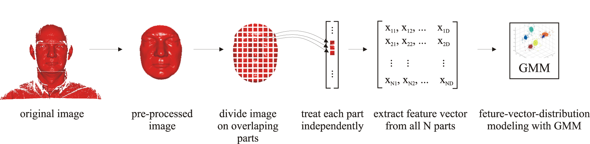
This section describes the basic characteristics of the 3D face recognition system used in the experimental section in conjunction with the classical GMM framework. First, data representation and its role in the recognition process are discussed. Next, the basics of DCT-based feature extraction in the GMM framework are reviewed and finally, the procedure of constructing user-specific GMMs and classifying them into client or impostor classes is presented. A schematic representation of the employed GMM framework can be seen in Figure 1.

Figure 1.

Conceptual diagram of the GMM framework

3.1 Data representation

There are several alternatives for representing facial data. Next to range images, a popular approach to represent 3D facial data is to consider differential geometry-based descriptors, such as curvature descriptors or surface normals. Curvature related descriptors are interesting due to their rotational invariance, which makes them a frequently used tool when segmenting 3D surfaces [31]. Surface normals are also suitable for the representation of facial data. Here, a surface normal is computed at each vertex of the facial surface and the x,y and z coordinates of the normals are used for data representation. Finally, one can also select angle values between surface normals and the average facial normal to represent the range image data.

Our preliminary experiments with different feature extraction and classification techniques have shown that angle values are best suited for 3D face data representation as they exhibit the highest level of robustness to different sources of data variability and among the above listed representations ensure the best recognition performance [32]. The experiments presented in Section 5 are, therefore, conducted on range images represented with relative angle values.

3.2 Feature extraction

Once a face representation is chosen, a set of feature vectors needs to be extracted from the computed data representation and fed to the GMM construction procedure. A popular tool for this task is DCT, which has proven to be suitable for block-based feature extraction from both, 2D images [33, 34] as well as 3D range images [5]. While several variants of DCT-based feature extraction techniques were presented in the literature (see for example [5, 34], all of them have the same initial stage consisting of analysing facial data block-by-block, with a configurable amount of overlap between neighbouring blocks. In this paper we use the most common variant of DCT-based feature extraction, where each individual image block is decomposed in terms of 2D DCT basis functions and the feature vector x belonging to the currently analysed block is formed by considering the first d DCT coefficients, i.e., x = [c_i]^d_i=0, where c_i is the i-th DCT coefficient.

3.3 Gaussian Mixture Models

GMMs are defined as a superposition of K Gaussian densities. They are used for modelling distributions of feature vectors and, therefore, serve as means for constructing user templates in biometric recognition systems. Parameters describing a GMM are mixing coefficients {π _k }^K_k=1, mean vectors {μ _k }^K_k=1 and covariance matrices {Σ _k }^K_k=1. Given a set of feature vectors {x _n }N_i=1, a GMM is constructed by determining its parameters λ = {π _k ,μ _k ,Σ _k }^K_k=1 based on the maximization of the following log-likelihood:

\log p (X | λ) = \sum_{n = 1}^{N} \log \sum_{k = 1}^{K} π_{k} N (x_{n} | μ_{k}, Σ_{k}),

(1)

where N is a Gaussian density function. Maximum likelihood (ML) solutions for the model parameters are found via the expectation-maximization (EM) algorithm [35] with k-means or Linde-Buso-Gray initialization.

When building user-specific GMMs, there is usually not enough data available to estimate the parameters of the GMM reliably. Therefore, a universal background model (UBM) is typically constructed first and then adapted with user-specific data. A UBM is itself a GMM representing generic, person independent feature characteristics. The parameters of the UBM are estimated via the ML paradigm (1) on all available training data. Once the UBM is built, user-specific GMM are computed via maximum a posteriori (MAP) adaptation. It has been observed that it is preferable to adapt only the means of the UBM. Therefore, the means for each user are adapted by iteratively evaluating the following expression [36]:

{\hat{μ}}_{k} = (1 - α) μ_{k} + α μ_{k}^{E M},

(2)

where ${\hat{μ}}_{k}$ is the new mean of the k -th Gaussian, μ _k is the mean from the previous step (initialized by the UBM) and μ _k ^EM is the re-estimated mean from the M-step of the EM algorithm. The parameter α balances the influence of the EM's new statistics and the prior mean μ _k .

3.4 Classification

Biometric verification systems based on statistical models typically use likelihood ratio based hypothesis testing to discriminate between legitimate users (or clients) and illegitimate users (or impostor). However, recent research suggest that better recognition results can be achieved by relying on support vector machines (SVM) [37, 38] for the classification task. Thus, we select SVMs as our classifiers and use them in all of our experiments. To be able to use SVMs for classification, the mean vectors of the user-specific GMMs are concatenated into equally sized supervectors and eventually used as inputs to the SVM classifier. During the enrolment stage, given a pool of supervectors from all training images and the client's supervector, the SVM training procedure constructs a decision hyperplane between the client's supervector and the training supervectors. At test time, the claimant's supervector is first derived by MAP adaptation and probability estimates are computed respective to the decision hyperplane learnt during the enrolment stage.

4. GMM framework modifications

In this section we present four possibilities of how to improve upon the classical GMM framework. The first three focus on considering the spatial structure of the face during the construction of the GMMs, while the last focuses on selecting only relevant features for modelling.

4.1 Using delta features

The first possibility for introducing spatial information into the classical GMM framework is to use delta coefficients (see Figure 2) and adding them to the commonly adopted DCT feature vectors [5, 34]. This modality will be referred to as GMMdel in the remainder of the paper.

Figure 2.

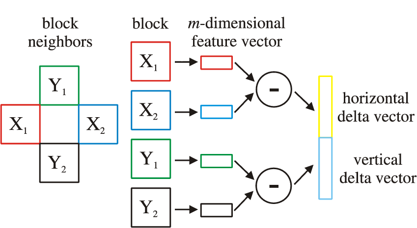
Conceptual diagram of DCT delta features extraction

Delta coefficients describe the dynamics between DCT coefficients of neighbouring image blocks and, therefore, introduce spatial dependencies into the feature vectors. When delta features are added to the feature vectors, each vector is implicitly linked to its (spatially) neighbouring feature vectors, resulting in a chain of dependencies. Consider two d -dimensional DCT feature vectors extracted from two (vertically or horizontally) neighbouring blocks of x _i , i.e., x_i-1 =[c_j(^i-1)]^d_j=0 and x_i+1 =[c_j⁽ⁱ⁺¹⁾]^d_j=0. The j -th delta coefficients can then be defined as follows:

Δ c_{j} = c_{j}^{(i + 1)} - c_{j}^{(i - 1)} .

(3)

In case the feature vectors x_i-1 1 =[c_j(^i-1)]^d_j=0 and x_i+1 = [c_j(ⁱ⁺¹⁾]^d_j=0 are extracted from vertically neighbouring blocks we obtain vertical delta coefficients and, similarly, if they are extracted from horizontally neighbouring blocks we obtain horizontal delta coefficients. It should be noted that delta coefficients are regularly used when building GMMs (see for example [34, 5]) and do not represent a novelty introduced in this paper. They are reviewed and assessed in this paper as they help to encode the spatial structure of the face into the GMM.

4.2 Constructing sub-image GMMs

The second possibility for considering the spatial structure of a face and, hence, for improving upon the classical GMM framework is by dividing the depth image into several (partially overlapping) sub-images and constructing a separate GMM for each sub-image [39] (see Figure 3). With this procedure, which will be denoted as GMMsub in the remainder, spatial constraints are enforced on the Gaussian mixtures, as each constructed GMM accounts only for a local region of the face.

Figure 3.

Schematic presentation of the GMMsub approach

In a similar manner as presented in Section 3.3, the sub-image GMMs are constructed, by first building a UBM for each sub-image from all available training data and adapting the UBM through MAP adaptation. The supervector, representing the input to our SVM classifier, is ultimately formed by a simple concatenation of the mean vectors of the computed sub-image GMMs.

4.3 Embedding positional information

The third possibility for introducing spatial information into the classical GMM framework is to embed the coordinates of the image block, from which the DCT feature vector is extracted, into the local feature vector itself and to form an augmented feature vector (see Figure 4). This modality, referred to as GMMext, accounts explicitly for the spatial position of the processed image blocks and results in feature vectors with two more elements, i.e.,:

x_{e x t} = {[x_{o r i g} a b]}^{T},

(4)

where x is the original feature vector and (a, b) are the coordinates of the upper left corner of the image block from which the feature vector was extracted.

Figure 4.

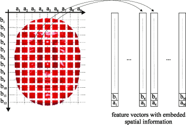
Conceptual example of augmented feature vectors

4.4 Removing least-likely feature vectors

Unlike the improvement possibilities presented above, the last possibility does not focus on introducing spatial information into the GMM framework, but instead focuses on the modelling procedure. When constructing GMMs based on the maximum likelihood criterion using either the EM or the MAP approach, all available feature vectors are generally taken into account. Or formally, all N feature vectors {x _n }^N_n=1 of an image are considered when evaluating (1). However, in cases where expression variations or shape artefacts are present in the (depth) face images, discarding image blocks belonging to facial areas that are most affected by such variations may lead to improved robustness and consequently improved recognition performance. The idea here is, when computing the likelihood of the features given a GMM, as in (1), the feature vectors with the lowest likelihood are likely to belong to areas deformed by expression variations, shape artefacts and the like. Therefore, the removal of these feature vectors and their exclusion from the GMM construction procedure can lead to improved robustness.

Given a set X = {x _n }^N_n=1 of N local feature vectors extracted from the given depth image and a GMM with parameters λ = {π _k , μ _k , Σ _k }^K_k=1, the following expression needs to be evaluated for each feature vector from the set X:

p (x_{n} | λ) = \sum_{k = 1}^{K} π_{k} N (x_{n} | μ_{k}, Σ_{k}) .

(5)

Based on the value of (5), a portion of feature vectors from X can be excluded from the GMM construction procedure. We will refer to this approach as GMMrem in the remainder of the paper.

5. Experiments

5.1 Data set and experimental protocol

In our experiments, we use the FRGC data set [40]. The face images in the FRGC data set have frontal view with minor pose variations and major expression variations. Images may contain shape artefacts such as deformed areas because of subjects moving during scanning, nose absence, holes, small protrusions and impulse noise (see Figure 5). The FRGC experimental protocol provides a set of standard verification experiments. The protocol defines three data sets -the training set, the gallery set and the probe set. The training set is used to build global face models. The gallery set contains images with known identities (intended for enrolment), while the probe set contains images with unknown identities presented to the system for recognition. Our experiments use the entire FRGC data set of 4007 range images belonging to 466 distinct subjects. We use only one enrolment image per client, so each image pair from the gallery and probe sets is considered independently, resulting in more than 16 million comparisons. Some experiments are also performed on a subset of the FRGC data (i.e., the FRGC version 1 data), where approximately 1 million comparisons are made.

Figure 5.

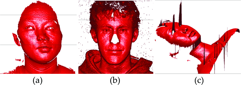
Sample images with artefacts from the FRGC data set: (a) deformed image, (b) nose absence, (c) impulse noise around the eyes

5.2 Data preprocessing

Images are initially low-pass filtered to remove spikes. The holes are filled using linear interpolation and finally the range data is smoothed with a mean filter. To test the robustness of the techniques assessed in our experiments for localization errors, we implement four different face localization procedures:

Meta-data localization (MD) - the technique uses the meta-data distributed with the FRGC data set for face localization, i.e., manually annotated eyes, nose tip and mouth coordinates, (see [41]),

ICP alignment (ICP) - the technique localizes the face scans by first roughly normalizing the position of the 3D faces based on the available meta-data and then employing the iterative closest point algorithm for fine alignment,

clustering-based background removal (BR) - the technique first removes the background of the 3D face scans and then clusters the remaining data into two clusters (head and body); from the two clusters the head cluster is easily identified (based on morphological characteristics) and used without any further alignment as input to the recognition techniques [26],

nose-tip alignment (NT) - the technique automatically detects the nose tip of the 3D faces and then crops the data using a sphere with radius r = 100 similar to [26].

Note that the first two techniques rely on manual annotation while the second two techniques are fully automatic and require no manual assistance. Examples of localized faces using the presented techniques are shown in Figure 6.

Figure 6.

Examples of face localization with the presented techniques

5.3 Experimental setup

There are a number of parameters regarding feature extraction, model training and classification that have to be properly set for optimal operation of the GMM framework. We set the parameters based on a simple optimization procedure over a small number of parameter settings and use the same settings for the proposed GMM modifications when making comparisons in the remainder of the paper.

Table 1 presents the verification performance of the classical GMM framework under different parameter settings. The parameter values in bold are also used in our following experiments. During the analysis of different block sizes and step sizes between neighbouring blocks, we observe that using smaller blocks leads to decreased performance, since features computed from small blocks are less descriptive due to limited surface variability. On the other hand, bigger block sizes result in a reduced number of observations per face, leading to a decreased performance as well. When studying the impact of the feature vectors size, we vary the length of our DCT feature vectors from 3 to 15. The best performance is achieved with a dimensionality of 15 and this value is also employed in our following comparative assessments, Note that increasing the number of considered DCT coefficients further does not have a significant effect on the recognition performance. The highest number of mixture components we examined was 512, where the best performance is achieved. In the following experiments, however, we use 256 mixtures to ease the computational burden.

Table 1.

Verification performance (TAR @ 0.1% FAR) of the classical GMM approach under different parameter settings

parameter	parameter setting / verification performance
block size (pixels)	20×20 / 92.4%	25×25 / 93.8%	30×30 / 95.2%	35×35 / 94.3%
step size (pixels)	3 / 96.4%	4 / 95.2%	5 / 89.1%	6 / 80.5%
feature vector length	3 / 73.1%	6 / 84.9%	10 / 90.6%	15 / 95.2%
number of mixtures	64 / 86.7%	128 / 90.9%	256 / 95.2%	512 / 95.9%

Other parameters that we use in our experiments are set as follows: EM steps: 15, number of MAP iterations: 3, relevance factor in MAP adaptation: 16, SVM kernel function: linear.

5.4 Experiment 1: Robustness to imprecise face localization

In our first series of experiments we assess the performance of the classical GMM framework. For this initial series of experiments we use the FRGCv1 data set.

To get an impression of the performance and robustness of the GMM framework in comparison with other techniques from the literature we implement the popular principal component analysis (PCA) [42] recognition technique as an example of holistic recognition methods and the recently proposed SIFT-based recognition approach from [12] as an example of local recognition procedures. We assess the performance of the three implemented techniques in conjunction with all four localization methods (described in the previous section) and present the results in the form of receiver operating characteristics (ROC) curves and true accept rates (TAR) at the false accept rate of 0.1%. Figure 7 shows the ROC curves of the experiments for each assessed method. As expected, all techniques perform best with the ICP algorithm, which ensures the best alignment of the faces, but also requires a decent initial alignment and requires the most time (as shown in Table 2). The MD approach ensures the second best results with all three recognition techniques, but requires manually annotated landmarks. Finally, the automatic techniques BR and NT produce the worst results of all techniques but are, on the other hand, robust, fast and require no manual assistance.

Table 2.

TAR at 0.1% FAR of the GMM, SIFT and PCA methods for different localization techniques

	BR	NT	MD	ICP
GMM	95.2%	97.0%	97.1%	97.5%
SIFT	80.9%	94.8%	95.8%	97.9%
PCA	16.5%	34.4%	41.0%	43.9%

Figure 7.

Experiment 1 ROC curves: robustness to imperfect normalization

If we look at Figures 7 and 8, and Table 2, where all techniques are compared in one place, we can actually see that the GMM framework was the least affected by localization and alignment imperfections. This fact is especially important when recognizing occluded 3D faces, where face alignment is particularly difficult [43].

Figure 8.

TAR at 0.1% FAR of all the assessed methods

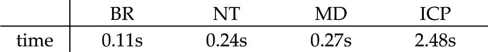
Table 3 denotes the average computational times for each of the assessed localization techniques. Time is reported for a single core of the 2.67 GHz Intel Xeon processor. All algorithms are implemented in MATLAB. We need to stress that the values in Table 3 should be taken with caution, as processing times depend heavily on the implementation.

Table 3.

Average running times of the assessed localization techniques

	BR	NT	MD	ICP
time	0.11s	0.24s	0.27s	2.48s

5.5 Experiment 2: Expression variation

Our second series of experiments examines the performance of the assessed algorithms in the presence of non-neutral facial expressions. For the experiments, images are partitioned into two sets depending on whether they exhibit neutral or non-neutral facial expression (expression labels provided by the FRGC protocol are used). All 943 images in the training set are classified as neutral, while in the gallery/probe set 2365 images are neutral and the remaining 1642 are non-neutral. The results of this series of experiments can be seen in Figure 9. The results clearly show that the GMM framework is the most robust for expression variations when compared to the SIFT and PCA approaches.

Figure 9.

Experiment 2 ROC curves: robustness to expression variation

5.6 Experiment 3: Time lapse between gallery and probe images

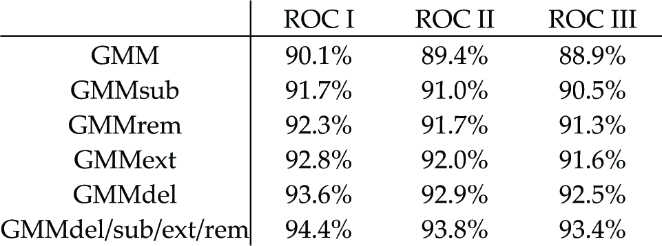
The third series of the experiments examines the performance of the assessed algorithms in the presence of a time lapse between gallery and probe images. Three ROC curves are generated, proposed by the FRGC versions 2 protocol. ROC I refers to images collected within a semester, ROC II refers to images collected within the same year and ROC III refers to images collected between semesters. These experiments are of increasing difficulty. The results of this series of experiments are presented in Figure 10. The results show that the GMM approach is the least affected by the presence of the time gap between gallery and probe images.

Figure 10.

Experiment 3 ROC curves: time lapse between gallery and probe images

5.7 Experiment 4: GMM modifications

In our final series of recognition experiments we use the data from FRGC version 2. Here, we evaluate the impact of the proposed GMM modifications on the face recognition performance. Note that this series of experiments is more challenging as more comparisons are made and both the probe, as well as the gallery, faces also feature expression variations. All parameters of the GMM framework are left as in the first series of experiments except for the number of GMM mixtures, which was increased to 512, since it was observed that an increased recognition performance is achieved with more mixtures. There are also some additional parameters in the GMMsub and GMMrem approaches that have to be set. For the GMMsub approach we examine several different ways of image partitioning. We chose to divide each image into 3 parts in the vertical and 2 parts in the horizontal direction of the face image, as the best recognition performance was obtained with this arrangement in our preliminary experiments. In the GMMrem approach we have to set the amount of low-likelihood features to be removed. Our preliminary experiments suggest that rejecting more than 10% of feature vectors has no additional positive effect on our results. Hence, we selected to reject 10% of least likely features.

First, we perform the all vs. all experiment, where every image from FRGC ver. 2 is compared to all the remaining images, resulting in 16052042 comparisons. The results of this series of experiments are presented in Figure 11. We can see that all the proposed GMM modifications result in improved performance when compared to the nonmodified GMM framework. All presented modifications can also be combined into a single system (denoted as GMMdel/sub/ext/rem for later convenience), which holds the properties of all the included modifications and outperforms all individual modifications assessed here.

Figure 11.

ROC curves of the GMM modifications (FRGC ver. 2, all vs. all data set, ICP localization)

To explore the robustness to imprecise face localization we assess the performance of each of the GMM modifications in conjunction with the four localization methods described in Section 5.2. The results of this series of experiments are presented in Table 4, where we can see that all the modifications result in improved performance. Similarly as in Section 5.4, the highest performance is achieved in conjunction with the ICP face localization, while the worst results belong to the experiments where the most imprecise BR localization is employed. We can also see that the GMMdel technique achieves the highest performance among all the assessed GMM modifications. Therefore, we conclude that the GMMdel modality most efficiently introduces the spatial information into the GMM framework. On the other hand the least improvement in performance is achieved with the GMMsub technique.

Table 4.

Robustness of the GMM modifications to imprecise localization (TAR @ 0.1% FAR, FRGC ver. 2, all vs. all data set)

	BR	NT	MD	ICP
GMM	87.0%	88.5%	88.7%	89.1%
GMMsub	87.4%	88.6%	89.1%	90.8%
GMMrem	88.9%	90.3%	90.6%	91.4%
GMMext	87.5%	89.9%	90.7%	91.8%
GMMdel	90.8%	91.2%	91.7%	92.7%
GMMdel/sub/ext/rem	91.0%	92.5%	92.9%	93.5%

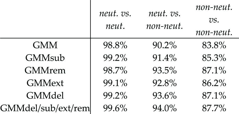
Next, we explore the robustness of GMM modifications to expression variations (see Table 6). Once again, we can see the improved performance of all the GMM modifications, except for the GMMrem approach in the case of the neutral vs. neutral data set. This behaviour is expected since neutral images do not contain many low-likelihoodfeature vectors, generally belonging to the areas with expression variations. The GMM modifications perform less well when matching the gallery and probe images across different facial expressions, however the drop in performance is relatively low when compared to the SIFT or PCA approaches (see Section 5.5).

Table 5.

Robustness of the GMM modifications in the presence of time lapse (TAR @ 0.1% FAR, FRGC ver. 2, ICP localization)

	ROC I	ROC II	ROC III
GMM	90.1%	89.4%	88.9%
GMMsub	91.7%	91.0%	90.5%
GMMrem	92.3%	91.7%	91.3%
GMMext	92.8%	92.0%	91.6%
GMMdel	93.6%	92.9%	92.5%
GMMdel/sub/ext/rem	94.4%	93.8%	93.4%

Table 6.

Robustness of the GMM modifications to expression variations (TAR @ 0.1% FAR, FRGC ver. 2, ICP localization)

	neut. vs. neut.	neut. vs. non-neut.	non-neut. vs. non-neut.
GMM	98.8%	90.2%	83.8%
GMMsub	99.2%	91.4%	85.3%
GMMrem	98.7%	93.5%	87.1%
GMMext	99.1%	92.8%	86.2%
GMMdel	99.2%	93.6%	87.1%
GMMdel/sub/ext/rem	99.6%	94.0%	87.7%

In the last set of experiments in this series we explore the robustness of the GMM modifications in the presence of a time delay between gallery and probe images. The results can be seen in Table 5. It can be deduced that all the GMM modifications contribute to an increased performance, while a slight decrease of the performance is noticed when the average time gap between gallery and probe images increases.

6. Conclusion

In this work the robustness of GMM-based 3D face verification systems in the presence of different sources of image variability is examined. The paper also discusses several different modifications of the classical GMM framework to improve its verification performance. We have evaluated how the assessed methods cope with imprecise face localization and facial appearance variations due to changes in expression. Using the FRGC database, we have shown that the performance of the GMM framework is significantly better than that of SIFT-based or PCA-based techniques and that the proposed modifications further improve its performance and robustness.

Footnotes

1

The probabilistic nature of GMMs makes it extremely easy to handle missing or corrupt data and to introduce hierarchical classification/modelling approaches.

7. Acknowledgments

The work presented in this paper was supported in parts by the national research program P2–0250(C) Metrology and Biometric Systems, the postdoctoral project BAMBI (ARRS ID Z2–4214), the joint Bulgarian research project entitled “Fast and reliable 3D face recognition” with ARRS ID Bi-Bg/11-12-007 and European Union's Seventh Framework Programme (FP7-SEC-2010–1) under grant agreement number 261727 (SMART).

References

Phillips

Scruggs

O'Toole

Flynn

Bowyer

Schott

and Sharpe

, “FRVT 2006 and ICE 2006 Large-Scale Experimental Results,” IEEE TPAMI, vol. 32, no. 5, pp. 831–846, 2010.

Anil

K. J.

Ross

and Prabhakar

, “An Introduction to Biometric Recognition,” IEEE TCSVT, vol. 14, no. 1, pp. 4–20, 2004.

Medioni

and Waupotich

, “Face Modeling and Recognition in 3-D,” Proc. of the AMFG, pp. 232–238, 2003.

Xiaoguang

and Jain

A. K.

, “Deformation Analysis for 3D Face Matching,” 7th IEEE Workshop on Applications of Computer Vision, vol. 1, pp. 99–104, 2005.

McCool

Sanchez-Riera

and Marcel

, “Feature distribution modelling techniques for 3D face verification,” Pattern Recogn. Lett., vol. 31, pp. 1324–1330, 2010.

Cook

Chandran

Sridharan

and Fookes

, “Face Recognition from 3D Data using Iterative Closest Point Algorithm and Gaussian Mixture Models,” Proc. of the 3DPVT, pp. 502–509, 2004.

Gonzales

R. C.

and Woods

R. E.

, Digital Image Processing, Addison-Wesley Longman, 1992.

Žibert

Pavešić

and Mhelič

, “Speech/non-speech segmentation based on phoneme recognition features,” EURASTP j. appl. signal process., pp. 1–13, 2006.

Scheenstra

Ruifrok

and Veltkamp

, “A Survey of 3D Face Recognition Methods,” Proc. of the AVBPA, pp. 891–899, 2005.

10.

Chang

Bowyer

and Flynn

, “A Survey of Approaches and Challenges in 3D and Multi-Modal 2D+3D Face Recognition,” Comput. Vis. Image Underst., vol. 101, no. 1, pp. 1–15, 2006.

11.

Kakadiaris

Passalis

Toderici

Murtuza

Karampatziakis

and Theoharis

, “Three-Dimensional Face Recognition in the Presence of Facial Expressions: An Annotated Deformable Model Approach,” IEEE TPAMI, vol. 29, no. 4, pp. 640–649, 2007.

12.

Inan

and Halici

, “3-D Face Recognition With Local Shape Descriptors,” Information Forensics and Security, IEEE Transactions on, vol. 7, no. 2, pp. 577–587, 2012.

13.

Man

Bennamoun

and Owens

, “An Efficient Multimodal 2D-3D Hybrid Approach to Automatic Face Recognition,” IEEE TPAMI, vol. 29, no. 11, pp. 1927–1943, 2007.

14.

Faltemier

Bowyer

and Flynn

, “A Region Ensemble for 3D Face Recognition,” IEEE Trans. on Information Forensics and Security, vol. 1, pp. 62–73, 2008.

15.

Hesher

Srivastava

and Erlebacher

, “A novel technique for face recognition using range imaging,” Proc. of the SPIA, vol. 2, pp. 201–204, 2003.

16.

Bronstein

and Kimmel

, “Expression-Invariant 3D Face Recognition,” Proc. of the AVBPA, pp. 62–70, 2003.

17.

Wang

Tan

and Quan

, “A New Attempt to Face Recognition using 3D Eigenfaces,” Proc. of the ACCV, pp. 884–889, 2004.

18.

Russ

Boehnen

and Peters

, “3D Face Recognition Using 3D Alignment for PCA,” Proc. of the CVPR, vol. 2, pp. 1391–1398, 2006.

19.

Colombo

Cusano

and Schettini

, “Gappy PCA Classification for Occlusion Tolerant 3D Face Detection,” J. Math. Imaging Vis., vol. 35, no. 3, pp. 193–207, 2009.

20.

Heseltine

Pears

in Austin

, “Three-Dimensional Face Recognition: A Fishersurface Approach,” Proc. of the ICIAR, zv. 2, pp. 684–691, 2004.

21.

Besl

and McKay

, “A Method for Registration of 3-D Shapes,” IEEE TPAMI, vol. 14, no. 2, pp. 239–256, 1992.

22.

and Siebert

, “Local feature extraction and matching on range images: 2.5D SIFT,” Comput. Vis. Image Underst., vol. 113, no. 12, pp. 1235–1250, 2009.

23.

Maes

Fabry

Keustermans

Smeets

Suetens

and Vandermeulen

, “Feature detection on 3D face surfaces for pose normalisation and recognition,” Proc. of the BTAS, pp. 1–6, 2010.

24.

Zhang

and Wang

, “Robust 3D face recognition based on resolution invariant features,” Pattern Recogn. Lett., vol. 32, no. 7, pp. 1009–1019, 2011.

25.

Szeptycki

Ardabilian

and Chen

, “A coarse-to-fine curvature analysis-based rotation invariant 3D face landmarking” Proc. of the BTAS, pp. 32–37, 2009.

26.

Segundo

M. P.

Queirolo

Bellon

O. R.

and Silva

, “Automatic 3D facial segmentation and landmark detection,” Proc. of the ICIAP, pp. 431–436, 2007.

27.

Irfanoglu

M. O.

Gokberk

and Akarun

, “3D Shape-based Face Recognition using Automatically Registered Facial Surfaces,” Proc. of the ICPR, pp. 183–186, 2004.

28.

Husken

Brauckmann

Gehlen

and Von der Malsburg

, “Strategies and Benefits of Fusion of 2D and 3D Face Recognition,” Proc. of the CVPR, pp. 174–179, 2005.

29.

Cardinaux

Sanderson

and Bengio

, “User Authentication via Adapted Generative Models of Face Images,” Signal Processing, IEEE Transactions on, vol. 54, pp. 361–373, 2006.

30.

Wang

Chua

and Ho

, “Facial feature detection and face recognition from 2D and 3D images,” Patt. Recogn. Letters, vol. 23, no. 10, pp. 1191–1202, 2002.

31.

Colombo

Cusano

and Schettini

, “3D Face Detection Using Curvature Analysis,” Pattern Recogn., vol. 39, pp. 444–455, 2006.

32.

Križaj

Štruc

and Dobrišek

, “Robust 3D Face Recognition,” Electrotehnical Review, article in press, 2012.

33.

Pennebaker

W. B.

and Mitchell

J. L.

, JPEG Still Image Data Compression Standard, Kluwer Academic Publishers, 1992.

34.

Sanderson

and Saban

, “On Local Features for GMM Based Face Verification,” Proc. of the ICITA, pp. 650–655, 2005.

35.

Moon

, “The expectation-maximization algorithm,” IEEE Signal Processing Magazine, vol. 13, no. 6, pp. 47–60, 1996.

36.

Reynolds

D. A.

Quatieri

T. F.

and Dunn

R. B.

, “Speaker verification using Adapted Gaussian mixture models,” Digital Signal Processing, vol. 10, pp. 19–41, 2000.

37.

Bredin

Dehak

and Chollet

, “GMM-based SVM for face recognition,” Proc. of the ICPR, pp. 1111–1114, 2006.

38.

Dornaika

Lazkano

and Sierra

, “Improving dynamic facial expression recognition with feature subset selection,” Pattern Recogn. Lett., vol. 32, no. 5, pp. 740–748, 2011.

39.

Zhen

and Huang

, “Spatial Gaussian Mixture Model for gender recognition,” Proc. of the ICIP, pp. 45–48, 2009.

40.

Phillips

P. J.

Flynn

P. J.

Scruggs

Bowyer

K. W.

Chang

Hoffman

Marques

Min

and Worek

, “Overview of the Face Recognition Grand Challenge,” Proc. of the CVPR, pp. 947–954, 2005.

41.

Chang

Bowyer

K. W.

and Flynn

, “An Evaluation of Multimodal 2D+3D Face Biometrics,” IEEE TPAMI, vol. 27, no. 4, pp. 619–624, 2005.

42.

Turk

and Pentland

A. S.

, “Face Recognition using Eigenfaces,” Proc. of the CVPR, pp. 586–591, 1991.

43.

Colombo

Cusano

and Schettini

, “UMB-DB: A database of partially occluded 3D faces,” Computer Vision Workshops (ICCV Workshops), pp. 2113–2119, 2011.

Towards Robust 3D Face Verification Using Gaussian Mixture Models

Abstract

Keywords

1. Introduction

2. Related work

2.1 Holistic methods

2.2 Local methods

3. Framework

3.1 Data representation

3.2 Feature extraction

3.3 Gaussian Mixture Models

3.4 Classification

4. GMM framework modifications

4.1 Using delta features

4.2 Constructing sub-image GMMs

4.3 Embedding positional information

4.4 Removing least-likely feature vectors

5. Experiments

5.1 Data set and experimental protocol

5.2 Data preprocessing

5.3 Experimental setup

5.4 Experiment 1: Robustness to imprecise face localization

5.5 Experiment 2: Expression variation

5.6 Experiment 3: Time lapse between gallery and probe images

5.7 Experiment 4: GMM modifications

6. Conclusion

Footnotes

1

7. Acknowledgments

References