Sage Journals: Discover world-class research

Abstract

The adaptive extended set-membership filter (AESMF) for nonlinear ellipsoidal estimation suffers a mismatch between real process noise and its set boundaries, which may result in unstable estimation. In this paper, a MIT method-based adaptive set-membership filter, for the optimization of the set boundaries of process noise, is developed and applied to the nonlinear joint estimation of both time-varying states and parameters. As a result of using the proposed MIT-AESMF, the estimation effectiveness and boundary accuracy of traditional AESMF are substantially improved. Simulation results have shown the efficiency and robustness of the proposed method.

Keywords

MIT-Rule ESMF Adaptive Estimation Mobile Robot

1. Introduction

Recently, improvements in the sequence estimation method make online real time modelling and control methods based on real time models feasible [1]. Among the statistical system estimation methods, the Kalman filter is the best known [2, 3, 4]. This filter is also known as a state estimator, utilizing the statistical knowledge of both the system measurement noise and the process noise – for instance, white noise – and achieves the optimal estimation by optimizing the minimum function of the estimation residuals. Also, its algorithm representation includes prediction and update, which is convenient in online applications. Hence, this method is widely used and it has been developed to the address nonlinear system estimation method and extends its application field, such as the extended Kalman filter (EKF) [5], the unscented Kalman filter (UKF) [6] and the derivative-free nonlinear Kalman filter [7], etc.

However, and generally, these Kalman filters require some statistical knowledge of the system measurement noise and process noise, or else assume that those noises meet some distributions in order to solve the optimal problems. However, in reality the system and environment noise characteristics are typically quite complicated, time varying, and difficult to measure and evaluate accurately. In particular, for robot systems, mechanical manufacture accuracy, sensory noise and air flow disturbances will result in uncertain statistical noises. The mismatch of the noise's statistical characteristics causes filter bias. Moreover, due to the Kalman filter's noise sensitivity, this bias is amplified and causes estimator instability. Therefore, many adaptive schemes – such as the adaptive unscented Kalman filter (AUKF) [8] – have been introduced to Kalman estimators in order to achieve the online noise estimation of the system's process noise distribution, and to compensate the filtering faults. However, the statistical dependency and sensitive nature of the Kalman estimator limits its system applications.

In most real systems, although the noise's statistical characteristics are unknown, they could be assumed as an unknown-but-bounded (UBB) noise. Due to the above defect of Kalman filtering, researchers have proposed a set-membership filter (SMF). Based on the UBB assumption, this filter gives a feasible state boundary by calculating the available set members. Thus, the estimation result is a viable state set rather than a single value. This viable state set describes possible ranges of the estimated parameters and makes sure that the real value falls in this set. At the end of the 1960s, ellipsoidal set-member filtering was first proposed by Schweppe [11] and Bertsekas [10]. They suggested deciding the real system state by applying the ellipsoidal geometric boundary. However, the optimization of the ellipsoid remained unconsidered. Later, Fogel and Huang [13] developed a nonlinear system optimal bounded ellipsoid (OBE) algorithm and then applied it to system identification. Maksarov [14], Kurzhanski [15] and Chernousko [16] improved and standardized the state and parameter ellipsoid estimation algorithm. Polyak [17] derived a linear system ellipsoid algorithm with model uncertainty, and it was extended to the present field of application.

Scholte and Campbell [18] expanded this ellipsoid algorithm into a nonlinear system and proposed an extended set-member filter (Extended SMF – ESMF). This follows the same mechanism for Kalman filtering by linearizing nonlinear systems. However, the difference is that ESMF uses Taylor expansion rather than nonlinear system linearization. This turns the linearization inaccuracy into the process noise in order to accomplish nonlinear system estimation. Yet, due to its numerical instability, poor real-time performance and difficulties in the tuning of the filter parameters, Zhou proposed a UD factorization-based adaptive extended set-membership filter (Adaptive ESMF – AESMF) [19] and overcame the flaw. This method represents and updates the envelope matrices using UD factorization; the method combines measurements in an updating strategy, which improves the algorithm's stability and reduces its complexity. Furthermore, as an adaptive filter parameter tuning method, it simplifies the algorithm complexity and search for the optimal results [20]. This method has been successfully applied in online modelling in robot systems.

However, the described method – the AESMF method – still requires the priori boundary information of the system noise. To be specific, this algorithm needs to know the uncertain boundaries of the process noise and measurement noise. Normally, measurement noise depends on sensory accuracy. If the sensors work under normal conditions, the uncertain boundary does not drift. Therefore, the sensor measurement uncertain boundary can be decided in advance by analyzing the measurement data; on the other hand, process noise comes from the mismatch between the system state space model and the systems' real dynamics, such as the parameters' mismatching. For most under-actuated and strongly-coupled nonlinear systems – such as robotic systems [22, 23, 24] – different operating modes result in a dissimilar dynamic model, even parameter transitions, which means that the system cannot be modelled accurately. Therefore, it is necessary to manually tune the boundary parameters since the priori information of uncertain boundaries are unknown. Meanwhile, as the priori knowledge is limited, manually setting the process noise uncertain boundary may not include or may well exceed the real process noise boundary. This will lead to the AESMF's estimated uncertain boundary being deviation too large, causing the filter to diverge during the estimation.

In this paper, a MIT-based AESMF (MIT-AESMF) is proposed to address the process noise uncertain boundary issue. This method applies MIT optimization rules and does online calculation to obtain the minimal ellipsoid boundaries of the prediction error, which also ensures that the filter's health-index satisfies the working condition. At the end, based on the MIT-AESMF method, an example of ground mobile robot state and dynamic parameter estimation proves the efficiency of this proposed method.

2. Traditional Adaptive Extended Set-Membership Filter (AESMF)

The main concept of AESMF is to cast the nonlinear dynamics in a way that allows the algorithm to take advantage of the linear SMF framework. Specifically, the nonlinear dynamics are linearized about the current estimation; the remaining terms are then proven bounded using interval analysis and are considered together with the process or measurement noises. Then, a linear SMF algorithm is used and an ellipsoid estimation set is achieved. The true value is guaranteed to lie in the ellipsoid.

The nonlinear system considered here has the following form:

x_{k + 1} = f (x_{k}) + w_{k}

(1)

y_{k + 1} = h (x_{k + 1}) + v_{k + 1}

(2)

where x_k ∈ Rⁿ and y_k+1 ∈ R^m are the state and measurement vectors, respectively, f(•) and h(•) are nonlinear C₂ functions, w_k ∈ Rn and v_k ∈ R^m are the process and measurement noise vectors, respectively, and they meet the conditions:

w_{k} \in E (0_{n \times 1}, Q_{k}), v_{k + 1} \in E (0_{m \times 1}, R_{k + 1})

where E(a, P) stands for an ellipsoid set as:

E (a, P) = {x \in R^{n} : {(x - a)}^{T} P^{- 1} (x - a) \leq 1}

where a is the centre, x is any point within the ellipsoid, and P is a positive-definite matrix.

The initial estimation ellipsoid is defined as:

x_{0} \in E ({\hat{x}}_{0}, P_{0})

where x̂ ₀ and P₀ stand for the initial estimation of the ellipsoid centre and envelope matrix, respectively. At time k, the estimated ellipsoid is defined as:

E_{k} = E ({\hat{x}}_{k}, P_{k})

Then, at time k+1, k=0, 1, 2,…, the AESMF algorithm [19] can be summarized as follows:

1. Calculate the state interval based on the ellipsoid extrema:

{\bar{X}}_{k}^{i} = [\begin{matrix} {\hat{x}}_{k}^{i} - \sqrt{P_{k}^{i, i}} & {\hat{x}}_{k}^{i} + \sqrt{P_{k}^{i, i}} \end{matrix}], i = 1, 2, \dots, n

(3)

where the superscript i, j stands for the (i, j) element of a matrix.

2. Find the maximum interval for the Lagrange remainder using the interval analysis: expanding the process function, Equation (1) (using one state as an example) yields:

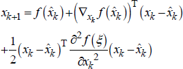
\begin{array}{l} x_{k + 1} = f ({\hat{x}}_{k}) + {(\nabla_{x_{k}} f ({\hat{x}}_{k}))}^{T} (x_{k} - {\hat{x}}_{k}) \\ + \frac{1}{2} {(x_{k} - {\hat{x}}_{k})}^{T} \frac{\partial^{2} f (ξ)}{\partial x_{k} ​^{2}} (x_{k} - {\hat{x}}_{k}) \end{array}

(4)

where ∇_xf is the gradient of the function, ∂² f / ∂x_k² is the second derivative of the function and £ can take any value on an interval X̄_k where (x_k – x̂_k) is defined. Then, the interval of the Lagrange remainder is defined as:

X_{R_{2}} (x_{k} - {\hat{x}}_{k}, {\bar{X}}_{k}) = \frac{1}{2} {(x_{k} - {\hat{x}}_{k})}^{T} \frac{\partial^{2} f ({\bar{X}}_{k})}{\partial x_{k}^{2}} (x_{k} - {\hat{x}}_{k})

(5)

Extending (9) to all states yields:

\begin{array}{l} X_{R_{2}} = \frac{1}{2} diag ({\bar{X}}_{k}^{T} - {\hat{x}}_{k}, {\bar{X}}_{k}^{T} - {\hat{x}}_{k}, \dots, {\bar{X}}_{k}^{T} - {\hat{x}}_{k}) \\ (\begin{matrix} H e s_{1} \\ \dots \\ H e s_{n} \end{matrix}) ({\bar{X}}_{k} - {\hat{x}}_{k}) \end{array}

(6)

where Hes_i, i =1, 2, …, n are the Hessian matrix of the nonlinear function f(•) and the interval vector X_k is now defined as X̄ = (X̄¹ _k , X̄_k²,…, X̄ⁿ_k).

3. Calculate the ellipsoid bounding the linearization error:

{[{\bar{Q}}_{k}]}_{R_{k}}^{i, i} = 2 {(X_{R_{2}})}^{2}, {[{\bar{Q}}_{k}]}_{R_{k}}^{i, j} = 0_{n \times 1} (i \neq j)

(7)

Then, the ellipsoid of linearization error is defined as E(0_n×1,Q̄_k).

4. Calculate the final process and linearization error bound ŵ_k ∈ E(0_nx1,Q̂_k):

{\hat{w}}_{k} \in E (0_{n \times 1}, {\hat{Q}}_{k}) \supseteq E (0_{n \times 1}, Q_{k}) \oplus E (0_{n \times 1}, {\bar{Q}}_{k})

(8)

where ŵ_k is the sum of the linearization error and w_k, and:

{\hat{Q}}_{k} = \frac{{\bar{Q}}_{k}}{1 - β_{Q_{k}}} + \frac{Q_{k}}{β_{Q_{k}}}, β_{Q_{k}} \in (0, 1)

(9)

where β_{Q_k} is a filter parameter to be chosen to minimize the ellipsoid E(0,Q̂_k). The observation model should be dealt with in the same way as with computing ŵ_k in Steps 2 – 4 to attain the incorporated measurement noise:

{\hat{v}}_{k + 1} \in E (0_{m \times 1}, {\hat{R}}_{k + 1})

5. Calculate the state prediction ellipsoid E(x̂_k+1,k,P_k+1,k) using the linear SMF filter, which is the direct sum of the predicted ellipsoid of the linearized model E(f(x̂_k), A_kP_kA_k^T) and the virtual noise ellipsoid E(0_nx1,Q̂_k):

{\hat{x}}_{k + 1, k} = f ({\hat{x}}_{k})

(10)

P_{k + 1, k} = Φ_{k} \frac{P_{k}}{1 - β_{k}} Φ_{k}^{T} + \frac{{\hat{Q}}_{k}}{β_{k}}, β_{k} \in (0, 1)

(11)

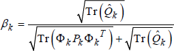
where β_k is a filter parameter to be chosen to minimize the ellipsoid E(x̂_k+1,k,P_k+1,k) and $Φ_{k} = \partial f (x_{k}) / \partial x_{k} | _{x_{k} = {\hat{x}}_{k}}$ is the Jacobian matrix of model (1).

6. Calculate the updated state ellipsoid E_k+1=E(x̂_k+1,P_k+1) using the linear SMF, which is the intersection of the predicted ellipsoid E(x̂_k+1,k,P_k+1,k)and the observation set $S_{y} = {x | {(y_{k + 1} - h (x))}^{T} {\hat{R}}_{k + 1}^{- 1} (y_{k + 1} - h (x)) \leq 1}$ :

W_{k} = H_{k + 1} \frac{P_{k + 1, k}}{1 - ρ_{k}} H_{k + 1}^{T} + \frac{{\hat{R}}_{k + 1}}{ρ_{k}}, ρ_{k} \in (0, 1)

(12)

K_{k + 1} = \frac{P_{k + 1, k}}{1 - ρ_{k}} H_{k + 1}^{T} W_{k} ​^{- 1}

(13)

{\hat{x}}_{k + 1} = {\hat{x}}_{k + 1, k} + K_{k + 1} [y_{k + 1} - h ({\hat{x}}_{k + 1, k})]

(14)

{\bar{P}}_{k + 1} = \frac{P_{k + 1, k}}{1 - ρ_{k}} - \frac{P_{k + 1, k}}{1 - ρ_{k}} H_{k + 1}^{T} W_{k} ​^{- 1} H_{k + 1} \frac{P_{k + 1, k}}{1 - ρ_{k}}

(15)

P_{k + 1} = δ_{k} {\bar{P}}_{k + 1}

(16)

where ρ_k is a filter parameter to be chosen to minimize the ellipsoid E(x̂_k+1,P_k+1), and δ_k is defined as:

δ_{k} = 1 - {[y_{k + 1} - h ({\hat{x}}_{k + 1, k})]}^{T} W_{k} ​^{- 1} [y_{k + 1} - h ({\hat{x}}_{k + 1, k})]

(17)

where $H_{k + 1} = \partial h (x_{k + 1}) / \partial x_{k + 1} | x_{k + 1} = {\hat{x}}_{k + 1, k} _{}$ is the Jacobian matrix of model (2).

For the selection of the parameters β_{Q_k}, β_k and ρ_k, reference [20] proposes the following adaptive strategy:

β_{Q_{k}} = \frac{\sqrt{Tr (Q_{k})}}{\sqrt{Tr ({\bar{Q}}_{k})} + \sqrt{Tr (Q_{k})}}

(18)

β_{k} = \frac{\sqrt{Tr ({\hat{Q}}_{k})}}{\sqrt{Tr (Φ_{k} P_{k} Φ_{k} ​^{T})} + \sqrt{Tr ({\hat{Q}}_{k})}}

(19)

ρ_{k} = \frac{\sqrt{r_{m}}}{\sqrt{p_{m}} + \sqrt{r_{m}}}

(20)

where p_m and r_m are maximum singular values of the matrix H_k+1 P_k+1,k H_k+1^T and R̂_k+1.

The update condition is given by reference [19] as:

{(y_{k + 1} - h ({\hat{x}}_{k + 1, k}))}^{T} {\hat{R}}_{k + 1}^{- 1} (y_{k + 1} - h ({\hat{x}}_{k + 1, k})) \leq η

(21)

where η ∈ R is a parameter to be selected. When this condition is not satisfied, only (10) and (11) are used to compute E(x̂_k+1,k, P_k+1,k) and stop computing (12)-(16). It has to be selected carefully, according to the initial assumption. Normally, larger η can increase the chance of not updating but will lead to larger estimation bounds. Namely, there is a trade-off between ‘update saving’ and conservative estimation.

Special attention should be given to the following two problems. First, when δ_k ≤ 0 in Equation (17), the uncertainty ellipsoid of Eq. (16) is not defined [19]. This will occur when the bound assumption (8) is not satisfied. That is, the practical state or noise is beyond the assumed bound. Thus, it provides an indication of the health of the algorithm. Second, the measurement noise bound R_k+1 can be decided through sensor calibration [25]. However, the process noise boundary Q_k, which comes from the model errors of the system (1) and which cannot be decided simply. Q_k is changed online and often selected by experience, while w_k^TQ_k⁻¹w_k = 1 is often assumed as the optimal condition as reference [20]. However, in real applications, model errors cannot be known accurately; thus, if the selected Q_k is much larger than real bounds, which means w_k^TQ_k⁻¹w_k « 1 and the estimated bound P will be much larger according to Eq. (11). This will result in an conservative estimation of state boundaries; if Q_k is much smaller than real bounds, which means w_k^TQ_k⁻¹w_k » 1, the estimated bound P will be much smaller according to Eq. (11, and no element can exist in the intersection of the predicted ellipsoid E(x̂_k+1,k,P_k+1,k) and the observation set $S_{y} = {x | {(y_{k + 1} - h (x))}^{T} {\hat{R}}_{k + 1}^{- 1} (y_{k + 1} - h (x)) \leq 1}$ .

This will result in δ_k ≤ 0, which means an unstable and undefined estimation.

In the following, a cost function is developed and a MIT adaptive strategy is introduced to solve the above two problems.

3. MIT-Based AESMF

As discussed above, the AESMF algorithm suffers from the mismatch of the process boundaries in practical usage. To solve this problem, a MIT adaptive strategy is introduced into the original AESMF algorithm to address the problem of the selection of Q_k online so as to ensure δ_k > 0.

Let q_kⁱ be the i-th diagonal element in Q_k, thus:

Q_{k} = d i a g {q_{k}^{1}, q_{k}^{2}, \dots, q_{k}^{n}}

(22)

According to the healthy index δ_k, the following optimized function is selected:

J_{k} (Q_{k}) = (1 - δ_{k}) • t r {P_{k + 1}}

(23)

where operator tr{*} is the trace of the matrix *.

Because tr{P_k+1}>0 and δ_k < 1, the cost function (23) is positive definite. Hence, based on the AESMF process (3–20), Q_k, which makes J_k(Q_k) minimal, and makes 1 – δ _k and tr{P_k+1} minimal at the same time. This means that the smallest boundaries of the estimated states set E(x̂_k+1,P_k+1) and δ _k → 1 are both guaranteed by:

Q_{k} = \underset{Q_{k}}{\arg \min} J_{k} (Q_{k})

(24)

Q_k must be the extreme point of J_k(Q_k) because J_k(Q_k) is positive definite, as discussed above. Thus, Q_k can be obtained by the following equation:

\frac{\partial J_{k} (Q_{k})}{\partial q_{k}^{i}} = t r {\frac{\partial (1 - δ_{k}) δ_{k} {\bar{P}}_{k + 1}}{\partial q_{k}^{i}}} = 0, i = 1, 2, \dots, n

(25)

However, in (25), W_k⁻¹ is included in δ_k and P̄_k+1, and W_k includes variable Q_k according to (11) and (12). This results in no analytic expressions for Q_k in (25). So, only a numerical solution can be obtained. We apply the MIT strategy [12] for the computation of Q_k as:

{\hat{q}}_{k + 1}^{i} = {\hat{q}}_{k}^{i} - Δ T • η_{k} \frac{\partial J_{k}}{\partial q_{k}^{i}} |_{q_{k}^{i} = {\hat{q}}_{k}^{i}}

(26)

where Q̂_kⁱ is the estimate of q_kⁱ at time k, ΔT is the sampling time, η _k is the parameter for the converge rate which is selected by hand and must satisfy the following condition:

{\begin{cases} η_{k} \geq 0 \\ \sum_{k} η_{k} = \infty \\ \sum_{k} η_{k}^{2} < \infty \end{cases}

(27)

According to (9), (11) and (12):

\begin{array}{l} \frac{\partial W_{k}}{\partial q_{k}^{i}} = \frac{\partial {H_{k + 1} \frac{P_{k + 1, k}}{1 - ρ_{k}} H_{k + 1}^{T} + \frac{{\hat{R}}_{k + 1}}{ρ_{k}}}}{\partial q_{k}^{i}} \\ = \frac{\partial {H_{k + 1} \frac{Φ_{k} \frac{P_{k}}{1 - β_{k}} Φ_{k}^{T} + \frac{\frac{{\bar{Q}}_{k}}{1 - β_{Q_{k}}} + \frac{Q_{k}}{β_{Q_{k}}}}{β_{k}}}{1 - ρ_{k}} H_{k + 1}^{T} + \frac{{\hat{R}}_{k + 1}}{ρ_{k}}}}{\partial q_{k}^{i}} \\ = \frac{\partial {H_{k + 1} \frac{Q_{k}}{β_{k} β_{Q_{k}} (1 - ρ_{k})} H_{k + 1}^{T}}}{\partial q_{k}^{i}} \\ = \frac{1}{β_{k} β_{Q_{k}} (1 - ρ_{k})} H_{k + 1} d i a g {\underset{i - 1}{\underset{︸}{0, \dots, 0}}, 1, \underset{n - i}{\underset{︸}{0, \dots, 0}}} H_{k + 1}^{T} \end{array}

(28)

\begin{array}{l} \frac{\partial {\bar{P}}_{k + 1}}{\partial q_{k}^{i}} \\ = \frac{\partial {\frac{P_{k + 1, k}}{1 - ρ_{k}} - \frac{P_{k + 1, k}}{1 - ρ_{k}} H_{k + 1}^{T} W_{k} ​^{- 1} H_{k + 1} \frac{P_{k + 1, k}}{1 - ρ_{k}}}}{\partial q_{k}^{i}} \\ = \frac{\partial {\frac{P_{k + 1, k}}{1 - ρ_{k}}}}{\partial q_{k}^{i}} - \frac{\partial {\frac{P_{k + 1, k}}{1 - ρ_{k}}}}{\partial q_{k}^{i}} H_{k + 1}^{T} W_{k} ​^{- 1} H_{k + 1} \frac{P_{k + 1, k}}{1 - ρ_{k}} \\ - \frac{P_{k + 1, k}}{1 - ρ_{k}} H_{k + 1}^{T} W_{k} ​^{- 1} \frac{\partial {W_{k}}}{\partial q_{k}^{i}} W_{k} ​^{- 1} H_{k + 1} \frac{P_{k + 1, k}}{1 - ρ_{k}} \\ - \frac{P_{k + 1, k}}{1 - ρ_{k}} H_{k + 1}^{T} W_{k} ​^{- 1} H_{k + 1} \frac{\partial {\frac{P_{k + 1, k}}{1 - ρ_{k}}}}{\partial q_{k}^{i}} \\ = \frac{1}{β_{k} β_{Q_{k}} (1 - ρ_{k})} {d i a g {\underset{i - 1}{\underset{︸}{0, \dots, 0}}, 1, \underset{n - i}{\underset{︸}{0, \dots, 0}}} \\ - d i a g {\underset{i - 1}{\underset{︸}{0, \dots, 0}}, 1, \underset{n - i}{\underset{︸}{0, \dots, 0}}} H_{k + 1}^{T} W_{k} ​^{- 1} H_{k + 1} \frac{P_{k + 1, k}}{1 - ρ_{k}} \\ - \frac{P_{k + 1, k}}{1 - ρ_{k}} H_{k + 1}^{T} W_{k} ​^{- 1} H_{k + 1} d i a g {\underset{i - 1}{\underset{︸}{0, \dots, 0}}, 1, \underset{n - i}{\underset{︸}{0, \dots, 0}}} \\ H_{k + 1}^{T} W_{k} ​^{- 1} H_{k + 1} \frac{P_{k + 1, k}}{1 - ρ_{k}} \\ - \frac{P_{k + 1, k}}{1 - ρ_{k}} H_{k + 1}^{T} W_{k} ​^{- 1} H_{k + 1} d i a g {\underset{i - 1}{\underset{︸}{0, \dots, 0}}, 1, \underset{n - i}{\underset{︸}{0, \dots, 0}}}} \end{array}

(29)

\begin{array}{l} \frac{\partial δ_{k}}{\partial q_{k}^{i}} = \frac{\partial {1 - {[y_{k + 1} - h ({\hat{x}}_{k + 1, k})]}^{T} W_{k} ​^{- 1} [y_{k + 1} - h ({\hat{x}}_{k + 1, k})]}}{\partial q_{k}^{i}} \\ = - \frac{1}{β_{k} β_{Q_{k}} (1 - ρ_{k})} {[y_{k + 1} - h ({\hat{x}}_{k + 1, k})]}^{T} W_{k}^{- 1} \\ H_{k + 1} \frac{\partial W_{k}}{\partial q_{k}^{i}} H_{k + 1}^{T} W_{k}^{- 1} {[y_{k + 1} - h ({\hat{x}}_{k + 1, k})]}^{T} \\ = - \frac{1}{β_{k} β_{Q_{k}} (1 - ρ_{k})} {[y_{k + 1} - h ({\hat{x}}_{k + 1, k})]}^{T} W_{k}^{- 1} \\ H_{k + 1} d i a g {\underset{i - 1}{\underset{︸}{0, \dots, 0}}, 1, \underset{n - i}{\underset{︸}{0, \dots, 0}}} \\ H_{k + 1}^{T} W_{k}^{- 1} {[y_{k + 1} - h ({\hat{x}}_{k + 1, k})]}^{T} \end{array}

(30)

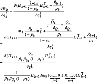
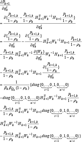
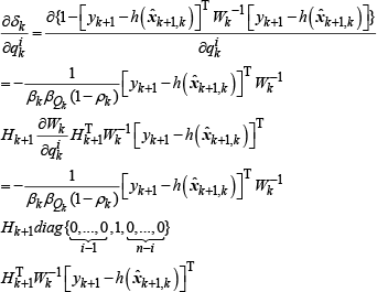
Hence the MIT strategy for estimation Q̂_kⁱ is:

\begin{array}{l} {\hat{q}}_{k + 1}^{i} \\ = {\hat{q}}_{k}^{i} - Δ T • η_{k} • t r {\frac{\partial (1 - δ_{k}) δ_{k} {\bar{P}}_{k + 1}}{\partial q_{k}^{i}}} \\ = {\hat{q}}_{k}^{i} - Δ T • η_{k} • t r {(1 - 2 δ_{k}) \frac{\partial δ_{k}}{\partial q_{k}^{i}} {\bar{P}}_{k + 1} + (1 - δ_{k}) δ_{k} \frac{\partial {\bar{P}}_{k + 1}}{\partial q_{k}^{i}}} \end{array}

(31)

Hence the MIT based AESMF method for model (1) and (2) is listed as following:

Initial conditions:

{\begin{cases} {\hat{q}}_{0}^{i} = q_{0}^{i} \\ Q_{0} = d i a g {{\hat{q}}_{0}^{1}, {\hat{q}}_{0}^{2}, \dots, {\hat{q}}_{0}^{n}} \\ {\hat{P}}_{0} = P_{0} \end{cases}

(32)

2. Construction of the noise boundaries at time k+1:

{\begin{cases} X_{k}^{i} = [\begin{matrix} {\hat{x}}_{k}^{i} - \sqrt{P_{k}^{i, i}} & , {\hat{x}}_{k}^{i} + \sqrt{P_{k}^{i, i}} \end{matrix}] \\ X_{R_{2}} = \frac{1}{2} diag (\underset{n}{\underset{︸}{X_{k}^{T} - {\hat{x}}_{k}, X_{k}^{T} - {\hat{x}}_{k}, \dots, X_{k}^{T} - {\hat{x}}_{k}}}) \\ (\begin{matrix} H e s_{1} \\ \dots \\ H e s_{n} \end{matrix}) (X_{k} - {\hat{x}}_{k}) \\ {[{\bar{Q}}_{k}]}_{R_{k}}^{i, i} = 2 {(X_{R_{2}})}^{2}, {[{\bar{Q}}_{k}]}_{R_{k}}^{i, j} = 0_{n \times 1} (i \neq j) \\ β_{Q_{k}} = \frac{\sqrt{Tr (Q_{k})}}{\sqrt{Tr ({\bar{Q}}_{k})} + \sqrt{Tr (Q_{k})}} \\ {\hat{Q}}_{k} = \frac{{\bar{Q}}_{k}}{1 - β_{Q_{k}}} + \frac{Q_{k}}{β_{Q_{k}}} \end{cases}

(33)

3. Time update at time k+1:

{\begin{cases} {\hat{x}}_{k + 1, k} = f ({\hat{x}}_{k}) \\ β_{k} = \frac{\sqrt{Tr ({\hat{Q}}_{k})}}{\sqrt{Tr (Φ_{k} P_{k} Φ_{k} ​^{T})} + \sqrt{Tr ({\hat{Q}}_{k})}} \\ P_{k + 1, k} = Φ_{k} \frac{P_{k}}{1 - β_{k}} Φ_{k}^{T} + \frac{{\hat{Q}}_{k}}{β_{k}} \end{cases}

(34)

4. Measure update at time k+1:

{\begin{cases} ρ_{k} = \frac{\sqrt{r_{m}}}{\sqrt{p_{m}} + \sqrt{r_{m}}} \\ W_{k} = H_{k + 1} \frac{P_{k + 1, k}}{1 - ρ_{k}} H_{k + 1}^{T} + \frac{{\hat{R}}_{k + 1}}{ρ_{k}} \\ K_{k + 1} = \frac{P_{k + 1, k}}{1 - ρ_{k}} H_{k + 1}^{T} W_{k} ​^{- 1} \\ {\hat{x}}_{k + 1} = {\hat{x}}_{k + 1, k} + K_{k + 1} [y_{k + 1} - h ({\hat{x}}_{k + 1, k})] \\ {\bar{P}}_{k + 1} = \frac{P_{k + 1, k}}{1 - ρ_{k}} - \frac{P_{k + 1, k}}{1 - ρ_{k}} H_{k + 1}^{T} W_{k} ​^{- 1} H_{k + 1} \frac{P_{k + 1, k}}{1 - ρ_{k}} \\ δ_{k} = 1 \\ - {[y_{k + 1} - h ({\hat{x}}_{k + 1, k})]}^{T} W_{k} ​^{- 1} [y_{k + 1} - h ({\hat{x}}_{k + 1, k})] \\ P_{k + 1} = δ_{k} {\bar{P}}_{k + 1} \end{cases}

(35)

5. Process noise boundaries update at time k+1:

{\begin{cases} {\hat{q}}_{k + 1}^{i} \\ = {\hat{q}}_{k}^{i} - Δ T • η_{k} • t r {(1 - 2 δ_{k}) \frac{\partial δ_{k}}{\partial q_{k}^{i}} {\bar{P}}_{k + 1} + (1 - δ_{k}) δ_{k} \frac{\partial {\bar{P}}_{k + 1}}{\partial q_{k}^{i}}} \\ Q_{k + 1} = d i a g {{\hat{q}}_{k + 1}^{1}, {\hat{q}}_{k + 1}^{2}, \dots, {\hat{q}}_{k + 1}^{n}} \end{cases}

(36)

where i = 1,2,..,n and j = 1,2,..,n.

4. Simulation

The proposed MIT-AESMF is tested by simulation to estimate the motion states and slip parameters of a tracked mobile robot, as shown in Figure 1. A general kinematics model of the tracked vehicle with consideration of slip is developed what follows. To compare the performance of MIT-AESMF with AESMF, this paper uses the same model for simulation with reference [20], in which AESMF is first proposed and tested.

Figure 1.

Platform of the Vehicle Undergoing General Planar Motion

In order to describe the motion of the tracked vehicle, define a fixed reference frame O_wX_wY_w and a moving frame O_mX_mY_m attached to the vehicle body, with an origin at the geometric centre of the vehicle. The motion of the vehicle is composed of the translation velocity V_c and the rotation velocity w_c=dψ / dt, where ψ is the yaw angle. Because of the sideslip, the instantaneous centre of rotation (ICR) shifts to the front of the vehicle centroid by d. The angle between the lines of Om-ICR and O'-ICR is defined as α, where O'-ICR is perpendicular to the axis X_m. Then, the discrete-time process model is:

\begin{array}{l} (\begin{matrix} X_{k + 1} \\ Y_{k + 1} \\ ψ_{k + 1} \end{matrix}) = (\begin{matrix} X_{k} \\ Y_{k} \\ ψ_{k} \end{matrix}) \\ + (\begin{matrix} \frac{r ω_{L} (1 - i_{L, k}) + r ω_{R} (1 - i_{R, k})}{2} (\cos ψ_{k} + σ_{k} \sin ψ_{k}) \\ \frac{r ω_{L} (1 - i_{L, k}) + r ω_{R} (1 - i_{R, k})}{2} (\sin ψ_{k} - σ_{k} \cos ψ_{k}) \\ \frac{- r ω_{L} (1 - i_{L, k}) + r ω_{R} (1 - i_{R, k})}{b} \end{matrix}) + w_{k} \\ = f (X_{k}, Y_{k}, ψ_{k}, i_{L, k}, i_{R, k}, σ_{k}) + w_{k} \end{array}

(37)

where X and Y are positions under the frame O_wX_wY_w, b is the distance between the midpoints of the two tracks, r is the radius of the wheels which drive the tracks, ΔT is the sampling interval, ω_L and ω_R are the angular velocities of the left and right wheels, i_L,k and i_R,k are the slip ratios of the left and right tracks. See reference [20] for the details of the dynamics of the robot.

In the simulations, X, Y and ψ are assumed as measurements. Thus, the observation model is:

y_{k} = {(\begin{matrix} X_{k} & Y_{k} & ψ_{k} \end{matrix})}^{T} + v_{k}

(38)

The goal of the simulation is to estimate the state (X_k Y_k Ψ_k) ^T and the three slip parameter vectors (i_L,k Y_L,k Ψ_L,k) ^T simultaneously. To solve this joint nonlinear estimation problem, a new augmented state vector is defined as the combination of the state and parameter vectors:

\begin{array}{l} x_{k} = {(x_{1, k}, x_{2, k}, x_{3, k}, x_{4, k}, x_{5, k}, x_{6, k})}^{T} \\ = {(\begin{matrix} X_{k} & Y_{k} & ψ_{k} \begin{matrix} i_{L, k} & i_{R, k} & σ_{k} \end{matrix} \end{matrix})}^{T} \end{array}

The slip parameters are often unknown in practice; hence, they are modelled as follows:

p_{k + 1} = p_{k} + w_{p,} ​_{k}

(39)

where p_k = (_L,k i_R,k σ_k) and w_p,k ∈ R³ is the additive process noise that drives the model (39). Thus, the joint-estimation equation is obtained [23] as:

{\begin{array}{l} x_{k + 1} \\ = (f (x_{1, k}, x_{2, k}, x_{3, k}, x_{4, k}, x_{5. k}, x_{6, k})) + (\begin{matrix} w_{k} \\ w_{p, k} \end{matrix}) \\ y_{k} = {(x_{1, k}, x_{2, k}, x_{3, k})}^{T} + v_{k} \end{array}

(40)

The constants in the model of Equation (40) are chosen as b=0.65m, r=0.35m, ΔT=100ms and ω_L= ω_R= 1.5 rad/s. The duration of the simulation is 200 sampling times (20s).

In order to demonstrate the tracking performance, step changes are simulated so as to occur in the three slip parameters (i_L,k Y_L,k ψ_L,k) at time k =100, which changes from (0.00 0.00 0.00) to (0.20 −0.10 0.15).

Assuming the real process noise w_k, the parameter driving noise w_p,k and the measurement noise v_k+1 are 5% equal distribution boundary noises. Assume the measurement noise is process noise and that v_k is the real boundary ellipsoid, R₀=diag{0.0025,0.0025,0.0025}. For every iteration, use x̂_k – the centre of the estimated ellipsoid E_k – as the estimated value of time step k.

In order to accurately compare and demonstrate the effectiveness of the filter, the state and parameter estimation accuracy in the least squares case is listed [20]:

V_{1} = \sqrt{\frac{1}{T} \sum_{t = 1}^{T} \sum_{i = 1}^{N_{x}} {(x_{i} (t) - {\hat{x}}_{i} (t))}^{2}}

(41)

V_{2} = \sqrt{\frac{1}{T} \sum_{t = 1}^{T} \sum_{i = 1}^{N_{p}} {(p_{i} (t) - {\hat{p}}_{i} (t))}^{2}}

(42)

V_{3} = \sqrt{\frac{1}{T} \sum_{t = 1}^{T} \sum_{i = 1}^{N_{p}} {({\bar{p}}_{i} (t) - {\underline{p}}_{i} (t))}^{2}}

(43)

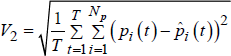
In the equations, x_i(t) and x̂_i(t) are real and estimated states, N_x is the dimension of the states, p_i(t) and p̂_i(t) are real and estimated parameters, N_p is the dimension of the parameters. p̄_i and p_i are the upper and lower boundary. The complexity of the different algorithms is described in terms of the CPU computing time. The health index recovering time is measured by the accumulation of the negative values.

In the following simulation, the normal AESMF and the proposed MIT-AESMF are compared in terms of stability, performance and computational load under the three conditions of the initial process boundary Q₀.

Condition 1:

The initial process noise ellipsoidal boundary is equal to the real boundary as:

Q_{0} = diag {0.0025, 0.0025, 0.0025, 0.0025, 0.0025, 0.0025}

Figure 2 depicts the estimation and stability improvement of MIT-AESMF. Figure 2-a is the estimation comparison of the system state Y_k, Figure 2-b is the comparison of the parameter i_L,k, Figure 2-c is the comparison of the filter health index δ _k . Figure 2 illustrates the fact that during the simulation the parameters and state estimates as well as the stable boundary estimation accuracy of both MIT-AESMF and AESMF are identical; however, because of the sudden changes, the initial ellipsoidal boundaries are far less than the parameter variations' equivalent process noise. Thus, the AESMF method employs this small ellipsoid in calculation, which causes the real value to be excluded from the estimation of the boundaries of the states and parameters, to fail the measure update requirements (21) and to stop the measurement updating. Ultimately, it causes uncertain boundaries to slowly inflate, and lasts for more than 10 sampling cycles until the boundaries include this sudden change range. Since the MIT-AESMF method adapts a MIT adaptive mechanism, it expands the process's ellipsoidal boundary to the entire sudden change range in 3 calculation cycles when a sudden parameter change occurs. Figure 2-c also demonstrates that when sudden change occurs, the MIT-AESMF health index uses 7 cycles less to return to 0 than the AESMF method. The comparisons of the performance of AESMF and MIT-AESMF are listed in Table 1 and Table 2.

Table 1.

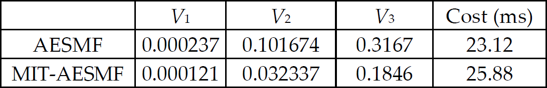
Performance of AESMF and MIT-AESMF (proper set-process boundaries and no parameter change)

	V ₁	V ₂	V ₃	cost (ms)
AESMF	0.000117	0.030884	0.1358	24.16
MIT-AESMF	0.000110	0.030657	0.1297	26.78

Table 2.

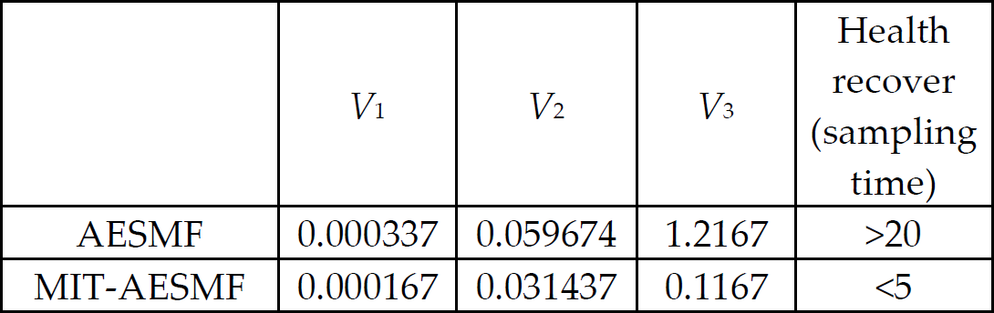
Performance of AESMF and MIT-AESMF following the step change of the parameters (proper set-process boundaries)

	V ₁	V ₂	V ₃	Health recover (sampling time)
AESMF	0.000337	0.059674	1.2167	>20
MIT-AESMF	0.000167	0.031437	0.1167	<5

Figure 2.

Performance comparison between AESMF and MIT-AESMF when the process noise boundaries equal the true value

According to Figure 2, Table 1 and Table 2, when the initial process noise ellipsoidal boundary equals the real boundary, and when compared to AESMF, MIT-AESMF displays similar parameter and boundary accuracy. However, when sudden change occurs, the estimation accuracy is bled and the health index is recovered in quite a short time, whereby the recovery speed is 5 time faster. MIT-AESMF is only 10% slower due to its online adaptive computing. These performances illustrate the adaptive ellipsoid MIT mechanism's effectiveness.

Condition 2:

The initial process noise ellipsoidal boundary is larger than the real boundary as:

Q_{0} = d i a g {0.01, 0.01, 0.01, 0.01, 0.01, 0.01}

Figure 3 depicts the estimation and stability improvement of MIT-AESMF. Figure 3-a is the estimation comparison of the system state Y_k, Figure 3-b is the comparison of the parameter i_L,k. Figure 3 illustrates that within the 200 points simulation, and besides 1 parameter's sudden change of moment,

Figure 3.

Performance comparison between AESMF and MIT-AESMF when the process noise boundaries are larger than the true value

MIT-AESMF and traditional AESMF have similar parameters and state estimation values. However, since the initial ellipsoidal boundary is set as too large, AESMF runs the calculation based on this big ellipsoid for the entire time, which leads to the states and parameter estimations' uncertain boundary being nearly twice as big as the MIT-AESMF method. This is mainly because the adaptive strategy of the MIT-AESMF method in the process noise ellipsoidal boundary estimation makes the real-time tuning of the ellipsoid boundary come close to the real process noise boundary. This result also implies that when the parameter's sudden change occurs, such as k=100, the MIT-AESMF method's noise adaptive mechanism makes Q_k closely approach the real boundary. Figure 3 clearly demonstrates, again, that because of the selective mechanism (21) in AESMF, when the parameter's sudden change happens, the initial process noise ellipsoidal boundary cannot include the span of the parameter variation and thereby causes the measurement to fail. Thus, just calculating the time update leads to the uncertain boundary's inflation, which remains for more than 20 sampling cycles until it includes the sudden change range, and the state estimation of AESMF becomes biased since there is no measurement updating. On the other hand, because the MIT-AESMF method adapts the MIT adaptive mechanism, which makes the process noise ellipsoidal boundary enlarge to the parameter of a sudden change range, it only takes 3 computing cycles whereas AESMF consumes about 20 or more cycles. Table 3 shows the comparison of the performance of the two filtering algorithms when the process noise ellipsoidal boundary is two times larger than the real boundary.

Table 3.

Performance of AESMF and MIT-AESMF (larger set-process boundaries)

	V ₁	V ₂	V ₃	Cost (ms)
AESMF	0.000237	0.101674	0.3167	23.12
MIT-AESMF	0.000121	0.032337	0.1846	25.88

According to Figure 3 and Table 3, when the initial process noise ellipsoidal boundary is twice as large as the real boundary, and compared to AESMF, MIT-AESMF has better accuracy and the parameter's uncertain boundary is about 1/2 that of the AESMF method during the estimation, which improves the effectiveness of traditional AESMF. Meanwhile, MIT-AESMF is only 10% slower due to its online adaptive computing.

Condition 3:

The initial process noise ellipsoidal boundary is smaller than the real boundary as:

Q_{0} = 10^{- 3} d i a g {0.625, 0.625, 0.625, 0.625, 0.625, 0.625}

Figure 4 describes the improvements in MIT-AESMF estimation and stability performance when the initial process noise ellipsoid is set as small. Figures 5-a and 5-b demonstrate that, in the 200 simulation moments, and because the initial ellipsoidal boundary is set too small, AESMF is using this small ellipsoid to calculate, which leads to no overlaps between the state estimation and the measurement estimation ellipsoids. Therefore, it does not satisfy AESMF's selective updating requirements (21), and at the same time the measurement updating makes the uncertain boundary shrink to the initial small ellipsoid boundary. Thus, there are no overlaps in measurement updating. This repeating process is shown clearly in Figure 4-c. Most of the time, the health index is far smaller than 0, and AESMF estimation is invalid, leading to the parameter and state estimation being both biased from the real value. In contrast, MIT-AESMF adapts the MIT adaptive mechanism in the process noise's ellipsoidal boundary estimation, and adjusts the process noise ellipsoidal boundary to approach the process noise's real value in real time, which causes MIT-AESMF to include the uncertain boundary of the real value, whereby the estimated noise boundary is twice as big as the valid AESMF estimated boundary (because of the mixing of the linearization error uncertain boundary and the measurement uncertain boundary – therefore, it does not exactly equal double the AESMF boundary). This feature corresponds with the initial 1/2 of the real process noise ellipsoidal boundary. This implies that the estimation of the process noise by using the MIT-AESMF method is close to the real value. The health index in Figure 4-c clearly shows that there is only a very short time for the health index to be less than 0, and it quickly recovers to 1 when a sudden change happens through using the MIT-AESMF method. This figure implies that the MIT-AESMF's estimation is guaranteed as valid. Table 4 shows the results of the two filtering methods when the initial process noise's ellipsoidal boundary is 1/2 of the real value.

Table 4.

Performance of AESMF and MIT-AESMF (smaller set-process boundaries)

	V ₁	V ₂	V ₃	Cost (ms)
AESMF	0.123123	0.183270	3.6138	20.12
MIT-AESMF	0.000188	0.028997	0.1755	25.68

Figure 4.

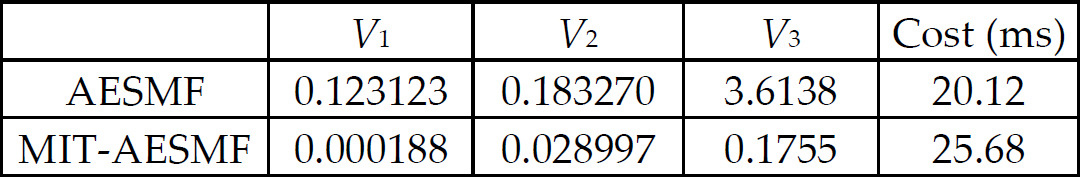
Performance comparison between AESMF and MIT-AESMF when the process noise boundaries are smaller than the true value

According to Figure 4 and Table 4, when the initial process noise ellipsoidal boundary is 1/2 of the real boundary, the original AESMF fails in making both the state and parameter estimation due to there being no overlaps in the prediction and measurement ellipsoids. Because of the selective updating mechanism, the filter is not valid for most of time. However, MIT-AESMF is effective for state and parameter estimation during the entire simulation, and maintains the same accuracy in Table 1. This implies that it is necessary to employ the MIT adaptive mechanism. Most of the time, AESMF does not perform measurement updating so that time is shortened when compared to Table 2. MIT-AESMF keeps the same time consuming level with Table 2.

To summarize MIT-AESMF and AESMF in the three scenarios. Although the proposed MIT-AESMF consumes 10% more computing time, when parameters suddenly change or the initial process noise boundaries are set larger or smaller than the real noise boundaries, it ensures that the estimation and the boundaries maintain the same accuracy as the original AESMF under ideal conditions. However, the traditional AESMF method generates a significant uncertain boundary estimation bias – estimation is even invalid under simulated conditions. Furthermore, in a situation such as where the health index is less than 0 due to system model being inaccurate, MIT-AESMF makes the health index recover faster its effective range, whereby the health index's recovery rate is close to 5 times that of the original AESMF method based on the selective method (21).

5. Conclusion

In this paper, a MIT-based adaptive set-membership filter is proposed for the joint state and parameter estimation of nonlinear systems. The normal AESMF is enhanced by the adaptive selection of the process noise boundaries based on the MIT adaptive strategy. This improves its effectiveness, realizes the optimal bound-guaranteed performance of the normal AESMF and does not increase the computation complexity. The proposed algorithms are presented and analysed in detail, and extensive simulations are carried out to perform the joint state and parameter estimation of a tracked mobile robot and to make comparisons between the normal AESMF and the proposed MIT-AESMF. It has been demonstrated that the proposed MIT-AESMF successfully solves the instability problem, realizes sub-optimal estimation and increases the estimation accuracy of the normal AESMF

Footnotes

6. Acknowledgments

This work was supported by The National Natural Science Foundation of China under Grant: 61035005, 61273025 and 61203334; National Key Technology R&D Program under Grant: 2011BAD20B07; National High Technology Research and Development Program (863) under Grant: 2012AA041501

References

Haykin

deFreitas

(2004) Special issue on sequential state estimation. Proceedings of the IEEE 92:399–400.

Ahrens

J.H.

Khalil

H.K.

(2007) Closed-loop behavior of a class of nonlinear systems under EKF-based control. Automatic Control, IEEE Transactions on 52:536–540.

Julier

S.J.

Uhlmann

J.K.

(2004) Unscented filtering and nonlinear estimation. Proceedings of the IEEE 92:401–422.

Park

Lee

Park

(2009) Correction Robot pose for SLAM based on Extended Kalman Filter in a Rough Surface Environment. International Journal of Advanced Robotic Systems 6:67–72.

Salvatore

Stasi

Tarchioni

(1993) A new EKF-based algorithm for flux estimation in induction machines. Industrial Electronics, IEEE Transactions on 40:496–504.

Julier

Uhlmann

Durrant-Whyte

H.F.

(2000) A new method for the nonlinear transformation of means and covariances in filters and estimators. Automatic Control, IEEE Transactions on 45:477–482.

Rigatos

G.G.

(2011) Derivative-Free Nonlinear Kalman Filtering for MIMO Dynamical Systems: Application to Multi-DOF Robotic Manipulators. International Journal of Advanced Robotic Systems 8:47–61.

Jiang

Song

Han

(2007) A novel adaptive unscented Kalman filter for nonlinear estimation. IEEE Conference on Decision and Control, New Orleans, USA. pp. 4293–4298.

Peng

Han

Huang

(2009) Adaptive UKF based tracking control for unmanned trimaran vehicles. International Journal of Innovative Computing, Information and Control 5:3505–3516.

10.

Bertsekas

Rhodes

(1971) Recursive state estimation for a set-membership description of uncertainty. Automatic Control, IEEE Transactions on 16:117–128.

11.

Schweppe

(1968) Recursive state estimation: Unknown but bounded errors and system inputs. Automatic Control, IEEE Transactions on 13:22–28.

12.

Song

Han

J.D.

(2008) An adaptive UKF algorithm for the state and parameter estimations of a mobile robot. Acta Automatica Sinica (English Version) 34:72–79.

13.

Fogel

Huang

Y.F.

(1982) On the value of information in system identification-bounded noise case. Automatica 18:229–238.

14.

Maksarov

Norton

(1996) State bounding with ellipsoidal set description of the uncertainty. International Journal of Control 65:847–866.

15.

Kurzhanski

A.B.

Varaiya

(2000) Ellipsoidal techniques for reachability analysis: Internal approximation. Systems & control letters 41:201–211.

16.

Chernousko

(2005) Ellipsoidal state estimation for dynamical systems. Nonlinear analysis 63:872–879.

17.

Polyak

B.T.

Nazin

S.A.

Durieu

Walter

(2004) Ellipsoidal parameter or state estimation under model uncertainty. Automatica 40:1171–1179.

18.

Scholte

Campbell

M.E.

(2003) A nonlinear set-membership filter for on-line applications. International Journal of Robust and Nonlinear Control 13:1337–1358.

19.

Zhou

Han

Liu

(2008) A UD factorization-based nonlinear adaptive set-membership filter for ellipsoidal estimation. International Journal of Robust and Nonlinear Control 18:1513–1531.

20.

Zhou

Han

J.D.

Liu

G.J.

(2007) An Enhanced Adaptive Set-Membership Filter for Nonlinear Ellipsoidal Estimation. American Control Conference.

21.

Zhou

Han

J.D.

(2007) Nonlinear Estimation Methods for Autonomous Tracked Vehicle with Slip: Compare Study. Chinese Journal of Mechanical Engineering (English Version) 20:1–7.

22.

Dierks

Jagannathan

(2010) Output feedback control of a quadrotor UAV using neural networks. Neural Networks, IEEE Transactions on 21:50–66.

23.

Song

D.L.

J.T.

Han

J.D.

Liu

G.J.

(2010) Active Modeling Based Predictive Control of Unmanned Helicopter in Full Flight Envelope. IEEE International Conference on Intelligent Robots and Systems: 616–621.

24.

Jung

Chung

(2011) Calibration of Kinematic Parameters for Two Wheel Differential Mobile Robots by Using Experimental Heading Errors. International Journal of Advanced Robotic Systems 8:134–142.

25.

Walker

D.K.

Randa

(2009) Variable Termination Unit for Noise-Parameter Measurement. Instrumentation and Measurement, IEEE Transactions on 58:1072–1077

26.

Song

Han

J.D.

(2008) An adaptive UKF algorithm for the state and parameter estimations of a mobile robot. Acta Automatica Sinica (English Version) 34:72–79.

A MIT-Based Nonlinear Adaptive Set-Membership Filter for the Ellipsoidal Estimation of Mobile Robots' States

Abstract

Keywords

1. Introduction

2. Traditional Adaptive Extended Set-Membership Filter (AESMF)

3. MIT-Based AESMF

4. Simulation

Condition 1:

Condition 2:

Condition 3:

5. Conclusion

Footnotes

6. Acknowledgments

References