Sage Journals: Discover world-class research

Abstract

We discuss a new design methodology for an inductive self-organizing network using an evolutionary algorithm and its practical applications. The inductive self-organizing network centres on the idea of a group method for data handling. The performances of this network depend strongly on the number of input variables available to the model and the number of input variables and type (order) of the polynomials to each node. They must be fixed by the designer in advance before the architecture is constructed. So the trial and error method must be used with its heavy computation burden and low efficiency. Moreover it does not guarantee that the obtained model is the best one. In this paper, we propose an evolutionary inductive self-organizing network to alleviate these problems. The order of the polynomial, the number of input variables and the optimum input variables are encoded as a chromosome and the fitness of each chromosome is computed. So the appropriate information for each node is evolved accordingly and tuned gradually throughout the genetic iterations. We can show that the proposed model is a sophisticated and versatile architecture which can construct models for limited data sets, as well as heavy complex robotic systems.

Keywords

Evolutionary algorithm inductive self-organizing network approximation and prediction abilities identification methods limited data set robotic system

1. Introduction

Group Method of Data Handling (GMDH) was introduced by Ivakhnenko in the early 1970s [1 -3]. GMDH-type algorithms have been extensively used since the mid-1970s for predicting and modelling complex nonlinear processes. The main characteristics of GMDH is that it is self-organizing and provides an automated selection of essential input variables without using prior information on the relationship between input-output variables [4]. A Self-organizing Polynomial Neural Network (SOPNN) is GMDH-type algorithm and one of the most useful approximator techniques [5]. SOPNN has an architecture similar to feed-forward neural networks whose neurons are replaced by polynomial nodes. The output of the each node in the SOPNN structure is obtained using several types of high-order polynomials such as linear, quadratic and modified quadratic of input variables. These polynomials are called Partial Descriptions (PDs). SOPNN have fewer nodes than NNs, but the nodes are more flexible. The SOPNN shows a superb performance in comparison to the previous fuzzy modelling methods. Although the SOPNN is structured using a systematic design procedure, it has some drawbacks which need to be solved. If there is a sufficiently large number of input variables and data points, the SOPNN algorithm has a tendency to produce overly complex networks. On the other hand, if a small number of input variables are available, SOPNN does not maintain good performance. Moreover, the performances of the SOPNN depend strongly on the number of input variables available to the model, as well as the number of input variables and polynomial types or order in each PD. They must be chosen in advance before the architecture of the SOPNN is constructed. In most cases, these are determined by the trial and error method with a heavy computational burden and low efficiency. Moreover, the SOPNN algorithm is a heuristic method so it does not guarantee that the obtained SOPNN is the best one for nonlinear system modelling. Therefore, more attention must be paid to solve the above-mentioned drawbacks.

In this paper we will present a new design methodology for SOPNNs using an evolutionary algorithm (EA) in order to alleviate the above-mentioned drawbacks. The presented network is applied to a 3-input nonlinear system and a humanoid robot which has heavy nonlinearity and complexity.

2. Evolutionary Inductive Self-organizing Network

In this section we will depict the evolutionary inductive self-organizing network (EISON) to be applied to 3-input nonlinear system and practical humanoid robot. Firstly the algorithm and its structure are shown and an evaluation of the usefulness of the method will follow.

2.1 Algorithm and structure

The EISON has an architecture similar to feed-forward neural networks whose neurons are replaced by polynomial nodes. The output of the each node in the EISON structure is obtained using several types of high-order polynomial such as linear, quadratic and modified quadratic of input variables. These polynomials are called Partial Descriptions (PDs). The PDs in each layer can be designed using evolutionary algorithms. The framework of the design procedure of the EISON comes as a sequence of the following steps.

[Step 1] Determine input candidates of a system to be targeted.

[Step 2] Form training and testing data.

[Step 3] Design partial descriptions and structure evolutionally.

[Step 4] Check the stopping criterion.

[Step 5] Determine new input variables for the next layer.

In the following, a more in-depth discussion on the design procedures, step 1~5, is provided.

Step 1: Determine input candidates

of a system to be targeted

We define the input variables such as x_1i, x_2i, ··· x_Ni related to output variables y_i, where N and i are the number of entire input variables and input-output data set, respectively.

Step 2: Form training and testing data

The input-output data set is separated into training (n_tr) data set and testing (n_te) data set. Obviously we have n = n_tr + n_te. The training data set is used to construct an EISON model and the testing data set is used to evaluate the constructed EISON model.

Step 3: Design Partial Descriptions (PD) and structure evolutionally

When we design the EISON, the most important consideration is the representation strategy, that is, how to encode the key factors of the PDs, order of the polynomial, the number of input variables and the optimum input variables, into the chromosome. We employ a binary coding for the available design specifications. We code the order and the inputs of each node in the EISON as a finite-length string. Our chromosomes are made of three sub-chromosomes. The first one consists of 2 bits for the order of polynomial (PD), the second one consists of 3 bits for the number of inputs of PD and the last one consists of N bits which are equal to the number of entire input candidates in the current layer. These input candidates are the node outputs of the previous layer. The representation of binary chromosomes is illustrated in Fig. 1.

Figure 1.

Structure of binary chromosome for a PD

The 1st sub-chromosome is made of 2 bits. It represents several types of order of PD. The relationship between bits in the 1st sub-chromosome and the order of PD is shown in Table 1. Thus, each node can exploit a different order of the polynomial.

Table 1.

Relationship between bits in the 1st sub-chromosome and order of PD.

Bits in the 1st sub-chromosome	Order of polynomial(PD)
00	Type 1 – Linear
10	Type 2 – Quadratic
11	Type 3 – Modified quadratic

The 3rd sub-chromosome has N bits, which are concatenated bits of0's and 1's coding. The input candidate is represented by a 1 bit if it is chosen as input variable to the PD and by a 0 bit it is not chosen. This way the problem of which input variables to be chosen is solved.

If many input candidates are chosen for the model design, the modelling is computationally complex and normally requires a lot of time to achieve good results. In addition, it causes improper results and poor generalization ability. Good approximation performance does not necessarily guarantee good generalization capability. To overcome this drawback, we introduce the 2nd sub-chromosome into the chromosome. The 2nd sub-chromosome consists of 3 bits and represents the number of input variables to be selected. The number based on the 2nd sub-chromosome is shown in Table 2.

Table 2.

Relationship between bits in the 2nd sub-chromosome and number of inputs to PD.

Bits in the 2nd sub-chromosome	Number of inputs to PD
000	1
001	2
010	2
011	3
100	3
101	4
110	4
111	5

Input variables for each node are selected among entire input candidates as many as the number represented in the 2nd sub-chromosome. The designer must determine the maximum number in consideration of the characteristic of the system, design specification and some prior knowledge of the model. With this method we can solve problems such as the conflict between overfitting and generalization and the requirement of a lot of computing time. The relationship between chromosome and information on PD is shown in Fig. 2. The PD corresponding to the chromosome in Fig. 2 is described briefly in Fig. 3.

Figure 2.

Example of a PD whose various pieces of required information are obtained from its chromosome

Figure 3.

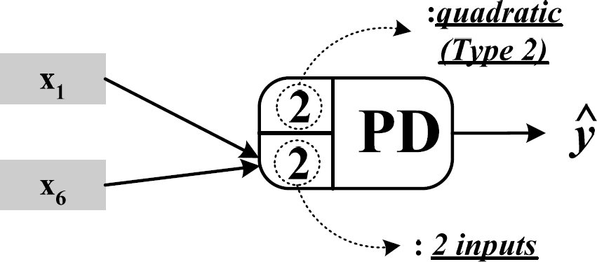
Node with PD corresponding to chromosome in Fig. 2.

Fig. 2 shows an example of the PD. The various pieces of required information are obtained from type of each chromosome. The 1st sub-chromosome shows that the polynomial order is Type 2 (quadratic form). The 2nd sub-chromosome shows two input variables to this node. The 3rd sub-chromosome tells that x₁ and x₆ are selected as input variables. The node with PD corresponding to Fig. 2 is shown in Fig. 3. Thus, the output of this PD, ŷ can be expressed as (1).

\hat{y} = f (x_{1}, x_{6}) = c_{0} + c_{1} x_{1} + c_{2} x_{6} + c_{3} x_{1}^{2} + c_{4} x_{6}^{2} + c_{5} x_{1} x_{6}

(1)

where coefficients c₀, c₁, …, c₅ are evaluated using the training data set by means of the standard least square estimation (LSE). Therefore, the polynomial function of PD is formed automatically according to the information of sub-chromosomes.

Step 4: Check the stopping criterion

The EISON algorithm terminates when the 3rd layer is reached.

Step 5: Determine new input variables for the next layer

If the stopping criterion is not satisfied, the next layer is constructed by repeating step 3 through to step 4.

The overall design procedure of the EISON is shown in Fig. 4. At the beginning of the process, the initial populations comprise a set of chromosomes that are scattered all over the search space. The populations are all randomly initialized. Thus, the use of heuristic knowledge is minimized. The assignment of a fitness function in the evolutionary algorithm serves as guidance to lead the search toward the optimal solution. The fitness function with several specific cases for modelling will be explained later. After each of the chromosomes is evaluated and associated with a fitness, the current population undergoes the reproduction process to create the next generation. The roulette-wheel selection scheme is used to determine the members of the new generation. After the new population is built, the mating pool is formed and the crossover is carried out. The crossover proceeds in three steps. First, two newly reproduced strings are selected from the mating pool produced by reproduction. Second, a position (one point) along the two strings is selected randomly. The third step is to exchange all characters following the crossing site. We use a one-point crossover operator with a crossover probability of P_c (0.85). This is then followed by the mutation operation. The mutation is the occasional alteration of a value at a particular bit position (we flip the states of a bit from 0 to 1 or vice versa). The mutation serves as an insurance policy which would recover the loss of a particular piece of information (any simple bit). The mutation rate used is fixed at 0.05 (P_m). Generally, after these three operations, the overall fitness of the population improves. Each of the population generated then goes through a series of evaluation, reproduction, crossover and mutation, and the procedure is repeated until a termination condition is reached. After the evolution process, the final generation of population consists of highly fit bits that provide optimal solutions. After the termination condition is satisfied, one chromosome (PD) with the best performance in the final generation of the population is selected as the output PD. All the remaining chromosomes are discarded and all the nodes that had no influence on this output PD in the previous layers are also removed. By doing this, the EISON model is obtained.

Figure 4.

Block diagram of the design procedure of the EISON.

2.2 Fitness function for the EISON

The important thing to be considered for the evolutionary algorithm is the determination of the fitness function. The genotype representation encodes the problem into a string, while the fitness function measures the performance of the model. It is quite important for evolving systems to find a good fitness measurement. To construct models with significant approximation and generalization ability, we introduce the error function such as

E = θ \times P I + (1 - θ) \times E P I

(2)

where θ ∈ [0,1] is a weighting factor for PI and EPI, which denote the values of the performance index for the training data and testing data, respectively, as expressed in equ. 5. The same performance index (Equ.(5)) is compared between the training and testing data sets as shown in Table 3. PI denotes a performance index of the model for the training data set, while EPI for the testing data. The proposed architecture, EISON model, has a weighting factor depicted in equ. 2. The weighting factor can be a certain number from 0 to 1, but only 5 cases [0.1, 0.25, 0.5, 0.75, 0.9] are considered in this paper. According to the weighting factor, conflict between over-fitting and generalization can be avoided. Inversely, the choice of weighting factor establishes a certain tradeoff between the approximation and generalization ability of the EISON. So the EISON outperforms the other models both in terms of accuracy and higher generalization capabilities. For a 3-input nonlinear system and robotic systems, 0.25 and 1 have best results, respectively. The fitness value is determined as follows:

Table 3.

Input-output data of 3-input nonlinear function.

Training data (1–20)						Training data (21–40)
No.	x ₁	x ₂	x ₃	x ₄	y	No.	x ₁	x ₂	x ₃	x ₄	y

1	1	3	1	1	11.11	21	1	1	5	1	9.545
2	1	5	2	1	6.521	22	1	3	4	1	6.043
3	1	1	3	5	10.19	23	1	5	3	5	5.724
4	1	3	4	5	6.043	24	1	1	2	5	11.25
5	1	5	5	1	5.242	25	1	3	1	1	11.11
6	5	1	4	1	19.02	26	5	5	2	1	14.36
7	5	3	3	5	14.15	27	5	1	3	5	19.61
8	5	5	2	5	14.36	28	5	3	4	5	13.65
9	5	1	1	1	27.42	29	5	5	5	1	12.43
10	5	3	2	1	15.39	30	5	1	4	1	19.02
11	1	5	3	5	5.724	31	1	3	3	5	6.38
12	1	1	4	5	9.766	32	1	5	2	5	6.521
13	1	3	5	1	5.87	33	1	1	1	1	16
14	1	5	4	1	5.406	34	1	3	2	1	7.219
15	1	1	3	5	10.19	35	1	5	3	5	5.724
16	5	3	2	5	15.39	36	5	1	4	5	19.02
17	5	5	1	1	19.68	37	5	3	5	1	13.39
18	5	1	2	1	21.06	38	5	5	4	1	12.68
19	5	3	3	5	14.15	39	5	1	3	5	19.61
20	5	5	4	5	12.68	40	5	3	2	5	15.39

F = \frac{1}{1 + E}

(3)

Maximizing F is identical to minimizing E.

3. Evaluation of the EISON

3.1 3-input nonlinear system

In this example, we will demonstrate how the proposed EISON model can be employed to identify the highly nonlinear function. The performance of this model will be compared with that of earlier works. The function to be identified is a 3-input nonlinear function given by (4)

y = {(1 + x_{1}^{0.5} + x_{2}^{- 1} + x_{3}^{- 1.5})}^{2}

(4)

which is widely used by Takagi and Hayashi[6], Sugeno and Kang[7], and Kondo[8] to test their modelling approaches. Table 3 shows 40 pairs of the input-output data obtained from (4) [9]. The data in Table 3 is divided into training data set (Nos. 1–20) and testing data set (Nos. 21–40). To compare the performance, the same performance index, average percentage error (APE) adopted in [6 -9] is used.

A P E = \frac{1}{m} \sum_{i = 1}^{m} \frac{| y_{i} - {\hat{y}}_{i} |}{y_{i}} \times 100 (%)

(5)

where m is the number of data pairs and y_i and ŷ_i are the i-th actual output and model output, respectively.

A series of comprehensive experiments was conducted and the results are summarized. The design parameters of the EISON in each layer are shown in Table 4.

Table 4.

Design parameters of the EISON for modelling.

Parameters	1st layer	2nd layer	3rd layer
Maximum generations	40	60	80
Population size:(w)	20:(15)	60:(50)	80
String length	8	20	55
Crossover rate (P_c)	0.85
Mutation rate (P_m)	0.05
Weighting factor: θ	0.1~0.9
Type (order)	1~3

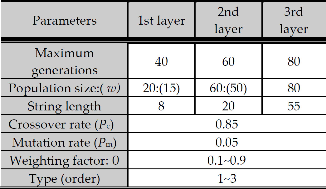
w: the number of chosen nodes whose outputs are used as inputs to the next layer. This number can be decided heuristically by the designer according to the uncertainty and nonlinearity of the target system.

The simulation results of the EISON are summarized in Table 5. The overall lowest values of the performance index, PI=0.188 EPI=1.087, are obtained at the 3^rd layer when the weighting factor (θ) is 0.25.

Table 5.

Values of performance index of the proposed EISON model.

Weighting factor	1st layer		2nd layer		3rd layer
Weighting factor	PI	EPI	PI	EPI	PI	EPI
0.1	5.7845	6.8199	2.3895	3.3400	2.2837	3.1418
0.25	5.7845	6.8199	0.8535	3.1356	0.1881	1.0879
0.5	5.7845	6.8199	1.6324	5.5291	1.2268	3.5526
0.75	5.7845	6.8199	1.9092	4.0896	0.5634	2.2097
0.9	5.7845	6.8199	2.5083	5.1444	0.0002	4.8804

Fig. 5 illustrates the trend of the performance index values produced in successive generations of the EA when the weighting factor θ is 0.25. Fig. 6 shows the values of error function and fitness function in successive EA generations when the θ is 0.25.

Figure 5.

Trend of performance index values with respect to generations through layers (θ =0.25)

Figure 6.

Values of the error function and fitness function with respect to the successive generations (θ =0.25).

Fig. 7 depicts the proposed EISON model with three layers when the θ is 0.25. The structure of the EISON is very simple and has a good performance. But for the conventional SOPNN from a few numbers of input candidates, it is impossible to structure the model for this nonlinear function.

Figure 7.

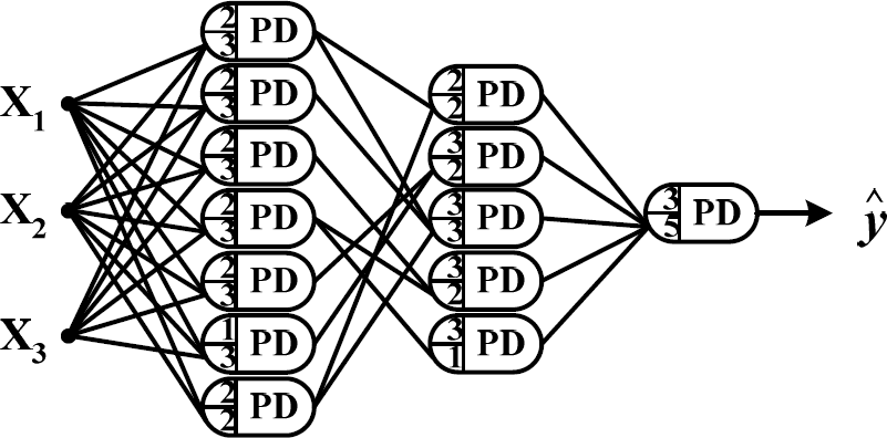
Structure of the EISON model with three layers (θ =0.25).

Fig. 8 shows the identification performance of the proposed EISON and its errors when the θ is 0.25. The output of the EISON follows the actual output very well.

Figure 8.

Identification performance of the EISON model with three layers and its errors.

Table 6 shows the performance of the proposed EISON model and other models studied in the literature. The experimental results clearly show that the proposed model outperforms the existing models both in terms of better approximation capabilities (PI), as well as superb generalization abilities (EPI). But the conventional model cannot be applied properly to the identification of this example.

Table 6.

Performance comparison of various identification models.

Model		APE
Model		PI (%)	EPI (%)
[7]	Model 1	1.5	2.1
[7]	Model 2	0.59	3.4
[8]		4.7	5.7
[9]	Type 1	0.84	1.22
	Type 2	0.73	1.28
	Type 3	0.63	1.25
[10]		2.11	1.54
[5]	Basic&Case1	2.59	8.52
[5]	Modified	Impossible
EISON		0.188	1.087

3.2 Practical biped humanoid robot

The bipedal structure is one of the most versatile ones for the employment of walking robots. The biped robot has almost the same mechanisms as a human and is suitable for moving in an environment which contains stairs, obstacle etc., where a human lives. However, the dynamics involved are highly nonlinear, complex and unstable. So it is difficult to generate a human-like walking motion. To realize human-shaped and human-like walking robots (humanoid robots), much research on biped walking robots has been conducted [11 -14]. In contrast to industrial robot manipulators, the interaction between the walking robots and the ground is complex. The concept of the zero moment point (ZMP) [12] is known to give good results in order to control this interaction. As an important criterion for the stability of the walk, the trajectory of the ZMP beneath the robot foot during the walk is investigated [11 -17]. Through the ZMP, we can synthesize the walking patterns of humanoid robot and demonstrate the walking motion with real robots. Thus, ZMP is indispensable to ensure dynamic stability for a biped robot. The ZMP represents the point at which the ground reaction force is applied. The location of the ZMP can be obtained computationally using a model of the robot, but it is possible that there is a large error between the actual ZMP and the calculated one, due to the deviations of the physical parameters between the mathematical model and the real machine. Thus, actual ZMP should be measured to realize stable walking with a control method that makes use of it.

In this paper, actual ZMP data throughout the whole walking phase are obtained from the practical humanoid robot and the EISON is applied. Joint angles, practical views and a block diagram of the implemented robot are shown in Fig. 9. The specifications of the biped robot are depicted in Table 7. The robot has 19 joints and height and weight are about 445mm and 3000g, respectively, including the vision camera. For the reduction of weight, the body is made of aluminium materials. Each joint is driven by the RC servomotor that consists of a DC motor, gear and simple controller. Each of the RC servomotors is mounted on the link structure.

Table 7.

Specifications of the robot.

Size	Height : 445mm
Weight	3kg
CPU	TMS320LF2407 DSP
Actuator (RC Servo motors)	HSR-5995TG (Torque : 30kg·cm at 7.4V)
Degree of freedom	19 DOF (Leg+Arm+Waist) = 26 + 32+1)
Power source	Battery
Actuator	: AA Size Ni-poly (7.4V, 1700mAh)
Control board	: AAA size Ni- poly (7.4V, 700mAh)

Figure 9.

Implemented humanoid robot, practical views and its block diagram.

As an important criterion for the stability of the walk, the trajectory of the ZMP beneath the robot foot during the walk is investigated. Through the ZMP, we can synthesize the walking patterns of a biped walking robot and demonstrate a walking motion with real robots. Thus, the ZMP is indispensable to ensure dynamic stability for a biped robot. The measured ZMP trajectory data to be considered here are obtained from 10 degree of freedoms (DOFs). Two DOFs are assigned to hips and ankles, and one DOF to the knee on both sides. From these joint angles, a cyclic walking pattern has been realized. This biped walking robot can walk continuously without falling down. The ZMP trajectory in the robot foot support area is a significant criterion for the stability of the walk. In many studies, the ZMP coordinates are computed using a model of the robot and information from the joint encoders, however, we employed a more direct approach which is to use measurement data from sensors mounted on the robot's feet.

The type of force sensor used in our experiments is FlexiForce sensor A201 which is shown in Fig. 10. They are attached to the four corners of the sole plate. Sensor signals are digitized by an ADC board, with a sampling time of 10 ms. Measurements are carried out in real-time. The foot pressure is obtained by summing the force signals. By using the force sensor data, it is easy to calculate the actual ZMP data. Feet support phase ZMPs in the local foot coordinate frame are computed by equ. 6

Figure 10.

Employed force sensors under the robot's feet.

P = \frac{\sum_{i = 1}^{8} f_{i} r_{i}}{\sum_{i = 1}^{8} f_{i}}

(6)

where f_i is each force applied to the right and left foot sensors, and r_i is sensor position which is vectored.

The walking motions of the biped humanoid robot are shown in Fig. 11. The figure shows a series of snapshots in the side views of the biped humanoid robot walking on a flat floor.

Figure 11.

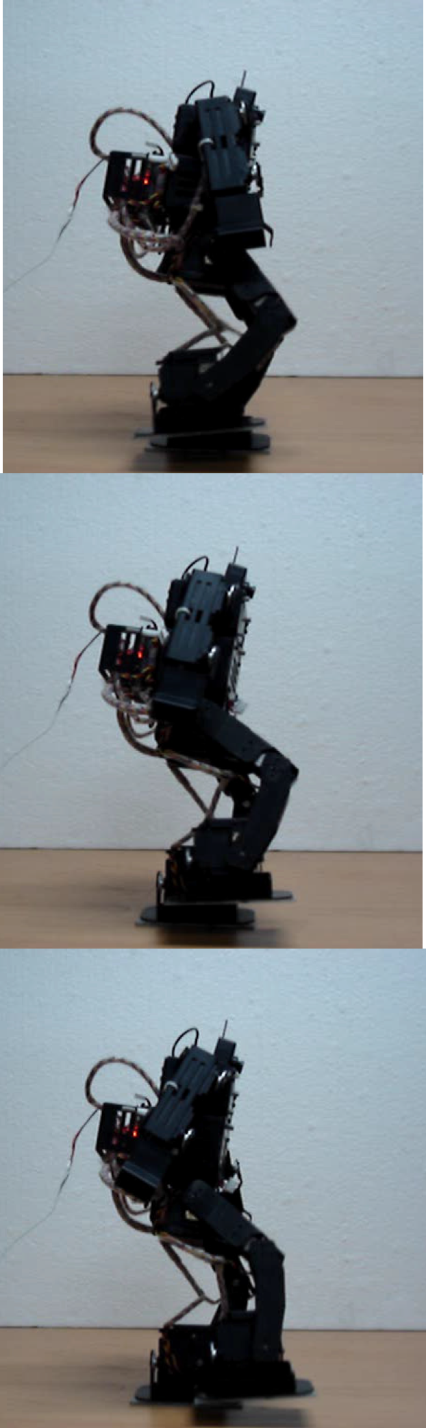
Side view of the biped humanoid robot on a flat floor.

Experiments using the EISON were conducted and the results are summarized in the tables and figures below. The design parameters of evolutionary inductive self-organizing network in each layer are shown in Table 8. The results of the EISON for the walking humanoid robot on the flat floor are summarized in Table 9. The overall lowest values of the performance indices, 6.865 and 10.377, are obtained at the 3^rd layer when the weighting factor (θ) is 1. In addition, the generated ZMP positions and corresponding ZMP trajectory are shown in Fig. 12.

Table 8.

Design parameters of the evolutionary inductive self-organizing network.

Parameters	1st layer	2nd layer	3rd layer
Maximum generations	40	60	80
Population size:(w)	40:(30)	100:(80)	160
String length	13	35	85
Crossover rate (P_c)	0.85
Mutation rate (P_m)	0.05
Weighting factor: θ	1
Type (order)	1~3

Table 9.

Condition and the corresponding MSE are included for the actual ZMP position in the four step motion of our humanoid robot.

Walking condition slope (deg.)	Layer	MSE (mm)
		x-coordinate	y-coordinate
0°	1	9.676	18.566
	2	7.641	13.397
	3	6.865	10.377

Figure 12.

Generated ZMP positions and corresponding ZMP trajectories.

4. Concluding remarks

In this paper, we propose a new design methodology for the EISON using evolutionary algorithms and the study properties of EISONs. We can see that the EISON is a sophisticated and versatile architecture which can construct models for limited data sets and complex humanoid robots. Moreover, the architecture of the model is not predetermined, but can be self-organized automatically during the design process. The example employed in the paper, a 3-input nonlinear system, is well modelled using the proposed method and we can get a reasonable approximation capability. In particular, the network size is smaller and the performance is better than the classical model. This could be possible due to two techniques combining optimization of evolutionary algorithms and polynomial approximation of SOPNNs. Occasionally, these good results can be varied according to the peculiarity of the system to be identified so this needs further research. The EISON model can be an effective means by which to construct a predictive model for poorly defined complex systems. According to the sophisticated and versatile architecture, the significance of these works is not restricted to a nonlinear static function. A humanoid robot is versatile and has almost the same mechanisms as a human – it is therefore suitable for moving in a human's environment – however, the dynamics involved are highly nonlinear, complex and unstable. It is therefore difficult to generate a human-like walking motion. In this paper, we have employed the zero moment point as an important criterion for the balance of the walking robots. In addition, the EISON is also utilized to establish empirical relationships between the humanoid walking robot and the ground, and to explain empirical laws by incorporating them into the humanoid robot. Thus, this work is significant for any complex process with nonlinearity.

Footnotes

5. Acknowledgments

This research was supported by the Basic Science Research Programme through the National Research Foundation of Korea (NRF) funded by the Ministry of Education, Science and Technology (grant no. 2011-0010579). Y-G Kim was supported by Ministry of Culture, Sports and Tourism and KOCCA in the CT R&D Program 2011.

References

Ivakhnenko

A. G.

, “Polynomial theory of complex systems”, IEEE Trans. Syst., Man, Cybern., Vol. SMC-1, No. 1, pp. 364–378, 1971.

Ivakhnenko

A. G.

and Ivakhnenko

N. A.

, “Long-term prediction by GMDH algorithms using the unbiased criterion and the balance-of-variables criterion,” Sov. Automat. Contr., Vol. 7, pp. 40–45, 1974.

Ivakhnenko

A. G.

Krotov

G. I.

and Ivakhnenko

N. A.

, “Identification of the mathematical model of a complex system by the self-organization method,” in Theoretical Systems Ecology: Advances and Case Studies, Halfon

, Ed. New York: Academic, 1970, ch. 13

Farlow

S. J.

, Self-Organizing Methods in Modeling, GMDH Type-Algorithms, New York: Marcel Dekker, 1984.

S. K.

and Pedrycz

, “The design of self-organizing Polynomial Neural Networks,” Inf. Sci., Vol. 141, pp. 237–258, 2002.

Takagi

and Hayashi

, “NN-driven fuzzy reasoning,” Int. J. Approx. Reasoning, Vol. 5, No. 3, pp. 191–212, 1991.

Sugeno

and Kang

G. T.

, “Structure identification of fuzzy model,” Fuzzy Sets Syst., Vol. 28, pp. 15–33, 1988.

Kondo

, “Revised GMDH algorithm estimating degree of the complete polynomial,” Tran. Soc. Instrum. Control Eng., Vol. 22, No. 9, pp. 928–934, 1986(in Japanese)

Horikawa

S. I.

Furuhashi

and Uchikawa

, “On Fuzzy modelling Using Fuzzy Neural Networks with the Back-Propagation Algorithm,” IEEE Trans. Neural Netw., Vol. 3, No. 5, pp. 801–806, 1992.

10.

M.J.

and Gao

, “A Fast Approach for Automatic Generation of Fuzzy Rules by Generalized Dynamic Fuzzy Neural Networks,” IEEE Trans. Fuzzy Syst., Vol. 9, No. 4, pp. 578–594, 2001.

11.

Erbatur

Okazaki

Obiya

Takahashi

Kawamura

, “A study on the zero moment point measurement for biped walking robots,” 7th International Workshop on Advanced Motion Control, pp. 431–436, 2002.

12.

Vukobratovic

Brovac

Surla

Stokic

, Biped Locomotion, Springer Verlag, 1990.

13.

Takanishi

Ishida

Yamazaki

Kato

, “The realization of dynamic walking robot WL-10RD,” Proc. Int. Conf. on Advanced Robotics, pp. 459–466, 1985.

14.

Hirai

Hirose

Haikawa

Takenaka

, “The development of Honda humanoid robot,” Proc. IEEE Int. Conf. on Robotics and Automation, pp. 1321–1326, 1998.

15.

Park

J. H.

Rhee

Y. K.

, “ZMP Trajectory Generation for Reduced Trunk Motions of Biped Robots,” Proc. IEEE/RSJ Int. Conf. Intelligent Robots and Systems, IROS '98, pp. 90–95, 1998.

16.

Park

J. H.

Cho

H. C.

, “An On-line Trajectory Modifier for the Base Link of Biped Robots to Enhance Locomotion stability,” Proc. IEEE Int. Conf. on Robotics and Automation, pp. 3353–3358, 2000.

17.

Kim

N.H.

Seo

S.J.

Park

G.T.

, “Fuzzy Modeling of Zero Moment Point Trajectory for a Biped Walking Robot,” Lect. Notes Artif. Int., vol. 3214, pp. 716–722, 2005 (awarded best paper)

Use of an Evolutionary Inductive Self-Organizing Network for Uncertain Nonlinear and Robotic Systems

Abstract

Keywords

1. Introduction

2. Evolutionary Inductive Self-organizing Network

2.1 Algorithm and structure

2.2 Fitness function for the EISON

3. Evaluation of the EISON

3.1 3-input nonlinear system

3.2 Practical biped humanoid robot

4. Concluding remarks

Footnotes

5. Acknowledgments

References