Micrometre Scale Performances of Industrial Robot Manipulators

Abstract

Robot precision is usually characterized by repeatability and accuracy. In this paper, we show that these indices are not sufficient to describe robot behaviour at the micrometre scale. New, precision performances are discussed and the experimental procedure to estimate these indices is described. The main results of the experimental work performed on Samsung Faraman and Epson Scara robots are displayed. Reversibility, hysteresis and spatial resolution have to be taken into account when the robot has to be controlled precisely at the micrometre scale. A granular control design including harmonization poses is proposed as a conclusion.

1. Introduction

The progress in robotics over recent years has extended our ability to explore, perceive, understand and manipulate the world on a variety of scales. In the fields of biology and surgery, the development of small robotics devices is rapidly increasing. In industry, applications of robotics at the micro-level include assembly [1–2], characterization, inspection and maintenance [3–4], micro-optics (the positioning of micro-optical chips) [5] and microfactories [6]. Many of these applications require the automated handling and assembly of small parts with accuracy within micron and sub-micron ranges. At the millimetre scale, robots can perfectly achieve most of these tasks but at the micrometre scale, the behaviour of the robot becomes unpredictable and is different from what is expected in theory. Many factors, including manufacturing and assembly tolerances, and deviations in actuator controllers, influence the precision performance index [7]. This is the reason why it is important to evaluate precision performances and develop innovative control strategies at the micrometre scale for industrial robots. This work will continue our investigation [8-11] about the micro displacements of serial robots. We study several aspects of micro movements enforced by the controller in order to increase our knowledge about the precision and repeatability of serial robots when performing micro tasks. We also propose some innovative strategies for the control and design of manipulators at the micrometre scale.

In the second section, the basic notations and studied robots are presented as well as the tests and experimental measurement device. In the third section, accuracy and repeatability are introduced and some results about orientation-repeatability are presented. The fourth section is concerned with reversibility, hysteresis, spatial resolution and the granularity of serial robots.

2. Manipulators and experimental device

When the robot holds a part and is controlled to place it very precisely, both position and orientation repeatabilities intervene, as Figure 1 illustrates. It is possible that some points of the solid part suffer from a misplacement whose cause comes mostly from orientation errors, dΩ, than from position errors, dG, of the mass centre.

Figure 1.

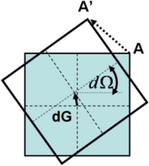
Misplacement of point A resulting from position and orientation errors

2.1 Definitions

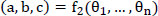
In order to control the joint angles according to the desired endpoint location and orientation, a kinematic model of the robot is required that involves many physical parameters, such as link lengths and joint offset angles. For manipulators with n joints, the forward kinematic model gives the function to compute the position and orientation of the end-effector from the angular variables of the joints θ_i, i = 1,…,n. Many industrial manipulators are composed of 6 joints in order to reach all positions and orientations in the workspace. The position is given by the variables (x, y, z) and the orientation is given by the variables (a, b, c):

$\left(\mathrm{x},\mathrm{y},\mathrm{z},\mathrm{a},\mathrm{b},\mathrm{c}\right)=\mathrm{f}({\mathrm{\theta }}_1,\dots ,{\mathrm{\theta }}_{\mathrm{n}})$

(1)

We can subdivide the function f into two functions f1 and f2 as:

$\left(\mathrm{x},\mathrm{y},\mathrm{z}\right)={\mathrm{f}}_1({\mathrm{\theta }}_1,\dots ,{\mathrm{\theta }}_{\mathrm{n}})$

(2)

$\left(\mathrm{a},\mathrm{b},\mathrm{c}\right)={\mathrm{f}}_2({\mathrm{\theta }}_1,\dots ,{\mathrm{\theta }}_{\mathrm{n}})$

(3)

From the functions f₁ and f₂, the position Jacobian matrix J_pos and orientation Jacobian matrix J_ori are defined to link the joint variations to the position and orientation variations. The Jacobian matrix J_pos is defined by (4):

${\mathrm{J}}_{\mathrm{p}\mathrm{o}\mathrm{s}}=\left[\frac{{\partial \mathrm{f}}_1}{{\partial \mathrm{\theta }}_1}\dots \mathrm{\hspace{0.17em}}\frac{{\partial \mathrm{f}}_1}{{\partial \mathrm{\theta }}_{\mathrm{n}}}\right]$

(4)

The orientation Jacobian matrix J_ori depends on the definition of angles a, b and c. When the roll – pitch – yaw (R, P, Y) angles are used, J_ori is computed from (5):

${\mathrm{J}}_{\mathrm{o}\mathrm{r}\mathrm{i}}=\left[\begin{array}{c}\left[\frac{\partial \mathrm{g}}{\partial {\mathrm{\theta }}_1}\dots \frac{\partial \mathrm{g}}{\partial {\mathrm{\theta }}_{\mathrm{n}}}\right]\times \left(\frac{1}{1+{\mathrm{g}}^2}\right)\\ \left[\frac{\partial \mathrm{h}}{\partial {\mathrm{\theta }}_1}\dots \frac{\partial \mathrm{h}}{\partial {\mathrm{\theta }}_{\mathrm{n}}}\right]\times \left(\frac{1}{1+{\mathrm{h}}^2}\right)\\ \left[\frac{\partial \mathrm{u}}{\partial {\mathrm{\theta }}_1}\dots \frac{\partial \mathrm{u}}{\partial {\mathrm{\theta }}_{\mathrm{n}}}\right]\times \left(\frac{1}{1+{\mathrm{u}}^2}\right)\end{array}\right]$

(5)

with [8]:

$\mathrm{g}=\tan \left(\mathrm{R}\right)=\frac{{\mathrm{M}}_{32}}{{\mathrm{M}}_{33}}$

(6)

$\mathrm{h}=\tan \left(\mathrm{P}\right)=\frac{{\mathrm{M}}_{21}}{{\mathrm{M}}_{11}}$

(7)

$\mathrm{u}=\tan \left(\mathrm{Y}\right)=\frac{{-\mathrm{M}}_{31}}{\sqrt{{{\mathrm{M}}_{11}}^2+{{\mathrm{M}}_{22}}^2}}$

(8)

and M = (M_ij) is the homogenous transformation matrix, which can be computed using the Khalil-Kleinfinger method [12-14]:

$\mathrm{M}={\mathrm{T}}_{\mathrm{0,1}}\times {\mathrm{T}}_{\mathrm{1,2}}\times \dots \times {\mathrm{T}}_{\mathrm{n}-1,\mathrm{n}}$

(9)

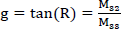
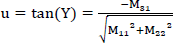
T_i,j is the transformation matrix modelling the displacement of coordinate frame j relative to coordinate frame i.

Joint variations affect the final position and orientation of the robot tool. The position and orientation Jacobian matrices map the angular small joint variations (dθ₁,…, dθ_n)^T with the tool position and orientation variations (dx, dy, dz)^T and (dR, dP, dY)^T according to Equations (10) and (11):

${(\mathrm{d}\mathrm{x},\mathrm{d}\mathrm{y},\mathrm{d}\mathrm{z})}^{\mathrm{T}}={\mathrm{J}}_{\mathrm{p}\mathrm{o}\mathrm{s}}\times {({\mathrm{d}\mathrm{\theta }}_1,\dots ,{\mathrm{d}\mathrm{\theta }}_{\mathrm{n}})}^{\mathrm{T}}$

(10)

${(\mathrm{d}\mathrm{R},\mathrm{d}\mathrm{P},\mathrm{d}\mathrm{Y})}^{\mathrm{T}}={\mathrm{J}}_{\mathrm{o}\mathrm{r}\mathrm{i}}\times {({\mathrm{d}\mathrm{\theta }}_1,\dots ,{\mathrm{d}\mathrm{\theta }}_{\mathrm{n}})}^{\mathrm{T}}$

(11)

Our research work is focused on repeatability modelling. We have proven in [11] that the angular variations can be modelled with a Gaussian distribution and that the density of position and orientation variables may be represented with stochastic ellipsoids [7-9].

2.2 Experimental measurement device

To estimate simultaneously the position and orientation variations of the end-effector, we use the stationary cube method proposed by the Ford Company, with six micrometres. The experimental measurement device consists of two trihedral parts. One is a parallelepiped moving with the robot and is held by the robot gripper. The other one is fixed on the robot base and supports those micrometres disposed orthogonally, as displayed in Figure 2.

Figure 2.

Measurement device with six micrometres

Three couples of micrometres are positioned on the sides of the fixed trihedral part. We chose this setup so as to keep the same resolution for the three orientation angles' estimation. Six 543–390 Mitutoyo micrometres are used to collect measurements. The accuracy is better than 3 micrometres and the resolution is 1 micrometre. With this device, it is possible to estimate the cube orientation with a resolution of 1.6×10⁻⁵ radians and the cube position with a resolution of 0.5 micrometres. The position and orientation variations are obtained from the six micrometre increments using a linear transformation from screw theory. The six micrometre values are read once the robot has reached its target and transferred to the PC via a multiplexor unit and the RS232 protocol.

2.3 Robot manipulators under study

The experiments are performed with two different manipulators. The first robot is a 6-axis Samsung Faraman robot, displayed in Figure 3. The kinematic architecture is a hybrid because there is a parallelogram for the second and third axes. The second robot is a 4-axis SCARA RS451 Epson robot, displayed in Figure 4. The robot has 4 degrees of freedom (DOF): three revolute joints (1, 2 and 4) and one vertical prismatic joint (3).

Figure 3.

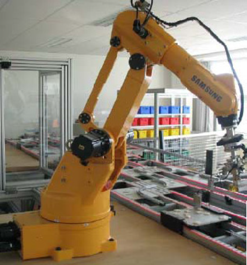
Samsung Faraman robot

Figure 4.

Epson RS451 SCARA robot

3. Repeatability and accuracy

Several methods are available for characterizing robot performance in accordance with the standards in [15–16]. The ISO9283 Standard describes a process to estimate positional and orientation precision indices. In the ANSI R15.05 Standard, estimation for position repeatability is given but nothing is offered concerning orientation precision [17–18]. According to the procedure proposed in the ISO9283 Standard, the robot endpoint is controlled to go to a specific position called “the target” and come back 30 times in the same conditions. When the robot reaches the target, the position and orientation of the robot tool are measured. Of course, the measured poses are not exactly the desired pose. There are small differences in the positions and orientations of the tool. Thus, they constitute a cloud of points. The precision indices described in the standard are built from this cloud and the desired pose.

3.1 Accuracy

“Accuracy” is the distance between the mean of the 30 final poses and the desired pose. This definition is used for position or orientation accuracy. The index depends, then, on the coordinate system used to measure the solid pose.

The position accuracy is the difference between the desired position of the robot endpoint and the barycentre of achieved positions, as displayed in Figure 5. It is given by (12):

Figure 5.

Position accuracy and repeatability (ISO 9283)

${\mathrm{A}\mathrm{P}}_{\mathrm{p}}=\sqrt{{\left({\mathrm{A}\mathrm{P}}_{\mathrm{x}}\right)}^2+{\left({\mathrm{A}\mathrm{P}}_{\mathrm{y}}\right)}^2+{\left({\mathrm{A}\mathrm{P}}_{\mathrm{z}}\right)}^2}$

(12)

where AP_x, AP_y and AP_z are the accuracies of position along the axes x, y and z:

${\mathrm{A}\mathrm{P}}_{\mathrm{x}}=\left(\stackrel{-}{\mathrm{x}}-{\mathrm{x}}_{\mathrm{c}}\right)$

(13)

${\mathrm{A}\mathrm{P}}_{\mathrm{y}}=(\stackrel{-}{\mathrm{y}}-{\mathrm{y}}_{\mathrm{c}})$

(14)

${\mathrm{A}\mathrm{P}}_{\mathrm{z}}=(\stackrel{-}{\mathrm{z}}-{\mathrm{z}}_{\mathrm{c}})$

(15)

x̄, ȳ, z̄ are the barycentre coordinates for the same pose repeated 30 times, and x_c, y_c and z_c are the coordinates of the controlled pose.

The orientation accuracy is the difference between the controlled orientation of the robot tool and the mean of achieved orientations, as displayed in Figure 6:

Figure 6.

Orientation accuracy and repeatability (ISO 9283)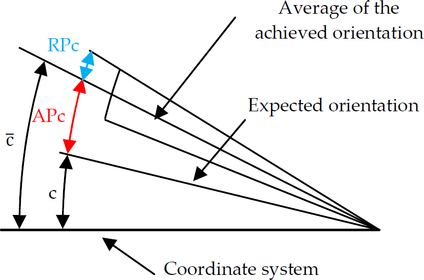

${\mathrm{A}\mathrm{P}}_{\mathrm{a}}=(\stackrel{-}{\mathrm{a}}-{\mathrm{a}}_{\mathrm{c}})$

(16)

${\mathrm{A}\mathrm{P}}_{\mathrm{b}}=(\stackrel{-}{\mathrm{b}}-{\mathrm{b}}_{\mathrm{c}})$

(17)

${\mathrm{A}\mathrm{P}}_{\mathrm{c}}=(\stackrel{-}{\mathrm{c}}-{\mathrm{c}}_{\mathrm{c}})$

(18)

where ā, b̄, and C̄ are the means of the angular variables for the same pose repeated 30 times, and a_c, b_c, and c_c are the angular coordinates of the controlled position.

3.2 Repeatability

The pose repeatability of a robot measures the variability or dispersion of the poses around the mean of the poses. The repeatability of position measures the dispersion between the final positions when the target is the same; the move is repeated several times. It is defined by (19):

${\mathrm{R}\mathrm{P}}_{\mathrm{L}}=\stackrel{-}{\mathrm{L}}+3{\mathrm{S}}_{\mathrm{L}}$

(19)

The random variable L is the distance from each position to the barycentre of the set. This random variable has a mean L̄ and a standard deviation S_L.

The repeatability of the orientation is defined as the range of angular variations ±3S_a, ±3S_b and ±3S_c around the mean values ā, b̄, and C̄:

${\mathrm{R}\mathrm{P}}_{\mathrm{a}}=\pm {3\mathrm{S}}_{\mathrm{a}}=\pm 3\sqrt{\frac{\sum _{\mathrm{j}=1}^{\mathrm{n}}{({\mathrm{a}}_{\mathrm{j}}-\stackrel{-}{\mathrm{a}})}^2}{\mathrm{n}-1}}$

(20)

${\mathrm{R}\mathrm{P}}_{\mathrm{b}}=\pm {3\mathrm{S}}_{\mathrm{b}}=\pm 3\sqrt{\frac{\sum _{\mathrm{j}=1}^{\mathrm{n}}{({\mathrm{b}}_{\mathrm{j}}-\stackrel{-}{\mathrm{b}})}^2}{\mathrm{n}-1}}$

(21)

${\mathrm{R}\mathrm{P}}_{\mathrm{c}}=\pm {3\mathrm{S}}_{\mathrm{c}}=\pm 3\sqrt{\frac{\sum _{\mathrm{j}=1}^{\mathrm{n}}{({\mathrm{c}}_{\mathrm{j}}-\stackrel{-}{\mathrm{c}})}^2}{\mathrm{n}-1}}$

(22)

S_a, S_b and S_c are the standard deviations related to the three angular coordinates of the achieved position.

3.3 Experimental estimation of repeatability

Using our measurement device, the orientation repeatability is estimated for the Samsung Faraman robot in 3 different locations – P1, P2 and P3 – in the workspace, as represented in Figure 7:

Figure 7.

Locations of P1, P2 and P3 in the workspace

• P1 (-80.7; 33.1; 20.1; −0.1; 69.4; 21.7): in the middle of the workspace

• P2 (-80.6; 68.3; 13.8; 0.2; 76.0; 19.5): very close to the workspace limit

• P3 (-90.0; −24.6; 37.6; 0.3; 53.2; 13.1): very close to the workspace centre (near the first axis)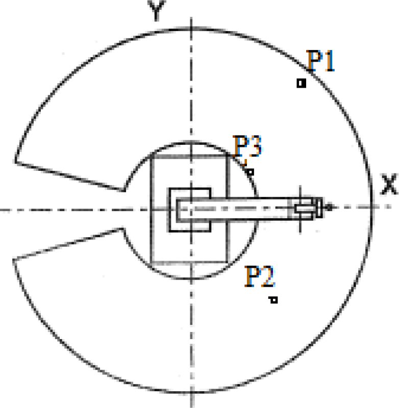

The repeatability was computed with 30 consecutive samples following the ISO92383. Then we compute 3 standard deviation confidence intervals with 6 series of 30 samples.

Table I displays the orientation repeatability values for the locations P1, P2 and P3 with a low (3kg) or high load (6kg).

Table 1.

Mean values (first row) and confidence intervals (second row) for orientation repeatability

Load (kg)	Locations	RPR (x10−5rad)	RPP (x10−5rad)	RPY (x10−5rad)
3	P1	5,67	6,91	3,91
		[3.26;8.07]	[3.61;10.2]	[2.65;5.17]
	P2	9.54	11.84	9.81
		[5.78;13.3]	[8.67;15.0]	[6.52;13.1]
	P3	20.54	22.17	20.74
		[4.57;36.5]	[8.43;35.9]	[9.47;32.0]
6	P1	7.16	8.50	8.19
		[4.86;9.46]	[5.90;11.1]	[6.41;9.97]
	P2	8.70	8.82	9.40
		[7.19;10.2]	[6.23;11.4]	[5.59;13.2]
	P3	11.61	16.10	11.88
		[6.21;17.0]	[11.2;21.0]	[7.25;16.5]

We present some comments concerning the results:

The influence of the load on the orientation repeatability is not very important. It appears, quite clearly, that the performance is better if the load is smaller, but the degradation is not really important when the load increases.

For a given location, the orientation repeatability is nearly the same for the three roll, pitch and yaw angles, and there is no special direction around which the result would be better.

The influence of the workspace location is not very important. It was not possible to notice significant differences. There are two main reasons for this result. First, the manufacturer's recommended workspace is not very large compared to the extended theoretical workspace, so it is difficult to choose a location significantly faraway. The second reason is the hybrid topological structure of the robot, which tends to unify repeatability in the workspace.

The variability of the results is important for all of the considered locations, but this variability is higher for P3. This location is, in fact, just outside the workspace recommended by the manufacturer. In fact, it seems that the robot cannot work efficiently in this location; it certainly has a link with the parallelogram structure of the 2^nd and 3^rd axes, which seem to be in a bad configuration if the end-effector stands in P3.

As a conclusion, the mean orientation repeatability is 12.5×10⁻⁵rad, whatever the location, angle or load. Let us also note that in our previous work we have presented a new approach to estimate the position and orientation repeatability indices with the angular covariance matrix. This procedure is cheap, simple and time saving, and it is based on the stochastic ellipsoid theory. We invite the readers to consider the references [7-11].

4. Reversibility, hysteresis and spatial resolution

In this section, we imagine that the robot is controlled to go to a target but, unfortunately, that the achieved position is not close enough to the target. What could we do to improve the final position? Usually, the error between the controlled and the achieved position is estimated and a new target is computed. This implies that the robot end-effector will move by small increments around the target. These increments could be in the same direction as the initial movement or in the inverse direction. Our research tries to quantify what could be done when small increments are controlled – i.e., at the scale of the angular resolution. The answer will result from the reversibility test, which will analyse the influence of the direction (left or right) and the hysteresis tests. Another strategy is to go backwards to a harmonization point and replay the whole trajectory, the target being slightly changed. The spatial resolution procedure will bring interesting results concerning this strategy.

4.1 Reversibility

There are several possible ways to reach a target. Considering a single joint i with an angular variable θ_i, the effector can reach the target coming from the left (L) or from the right (R). It is well-known that the direction will affect the mean of the distribution. This phenomenon is – most of the time – called “backlash in the gear reductor box” or else “hysteresis”. The goal of the algorithm described below is to estimate the difference between the means of the two final distributions. Once this difference is stochastically known, it is possible to build a strategy to reduce the final position error in the next attempt, taking into account the direction of the movement. The procedure consists of repeating, 15 times, the following cycle:

1. The robot comes from a left harmonization point θ_i^L,

2. It goes to the measurement point θ_i^M,

3. It goes to the right harmonization point θ_i^R,

4. It comes back to the measurement point θ_i^M.

This algorithm is applied to the first axis of the Epson Robot. The left and right harmonization points are situated symmetrically and at a short distance from the measurement point, as illustrated in Figure 8. This cycle is repeated N = 15 times, such that we have N measurements corresponding at a target attained coming from the left-side and N measurements coming from the right-side. The measurements are provided in radians. The angular acceleration is set to 3% of the maximal acceleration. When the first axis moves, the second axis also moves due to the dynamical effects. As such, it is necessary to use at least two micrometres to estimate simultaneously the first and second axes' variations.

Figure 8.

Reversibility estimation procedure

Figure 9 displays the measured positions when the robot comes from the left (first axis: upper curve in a continuous line; second axis: lower curve in a continuous line) or from the right (first axis: upper curve in a dotted line; second axis: lower curve in a dotted line). First, it can be seen that when only one arm is controlled to move, the other arm also moves. This can be easily understood because there is no brake – neither on the first nor the second axis. Consequently, when, the first axis is moving, the second axis's position is controlled by the regulation loop only. The torque resulting from the dynamical effects tends to create an error in the position regulation loop. This error is then corrected and is nil at the end of the process, but the second axis has then moved.

Figure 9.

Angular positions in the reversibility procedure

For the first axis, the left curve is always over the right one, meaning that there is a steady bias if the target is hit coming from L or from R. This bias is statistically significant. For the second axis, the right curve is always under the left one, meaning that there is a steady bias, concerning the second axis's position. There is also an inverse correlation between the two axes' positions. This could be explained by the fact that the first motor is set on the robot's base while the second motor is set on the second link. The first link does not support any motor. Thus, the reductors have opposite effects on the links.

4.2 Hysteresis

Sometimes, when the robot is controlled to perform a small jump, no movement is measured. Meanwhile the motor has moved, which is observed via the incremental encoders. However, the solid friction and elasticity of the reductor prevent the cube from moving. We tried to perform experiments to characterize the minimal incremental value that would produce a movement at the end of the kinematic chain. The idea is to control each joint to move in small increments from a given position and measure the displacements at the end of the kinematic chain. The robot is controlled to increase and decrease angular positions by increments of n pulses, n=1 to 7, as detailed in Figure 10 where T is the target.

Figure 10.

Hysteresis procedure

This procedure is applied to the first and second axis of the Epson Robot. Table 2 sums up the results for the hysteresis measurements. For the joint, the mean value dθ_i / n / res i is reported with respect to the number of pulses n. The first axis's theoretical resolution is res1 = 1.92×10⁻⁵ rad and the second axis's theoretical resolution is res2 = 3.07×10⁻⁵ rad. The measurements are provided as percentages.

Table 2.

Hysteresis performances

n	dθ1 / n/res1×100	dθ2 / n/res2×100
1pls	73	10
2pls	55	16
3pls	60	56
4pls	76	71
5pls	93	79
6pls	93	84
7pls	100	87

The experimental results show that it is impossible to directly move the robot by one pulse. Moreover, when two or more pulses are controlled, there is also a nonlinearity that should be taken into account.

4.3 Spatial resolution

The robot's i^th axis is controlled to reach a position θ_i0 associated with target T coming from a harmonization point HP associated with target T_HP. The final position is measured. Then, the robot comes back to HP and the next target will be θ_i0+1 pulse. The final position is measured. The cycle is repeated again with a new target θ_i0+2 pulses, and so on, as displayed in Figure 11.

Figure 11.

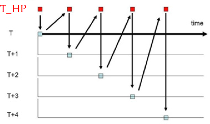
Spatial resolution procedure

As illustrated in Table 3, the spatial resolution can be considered to be statistically independent of the number of pulses. This last experiment points to the interest in introducing a harmonization point in the control design of micrometre movements.

Table 3.

Spatial resolution performances

n	dθ1 / n /res1×100	dθ2 / n/res2×100
1pls	100	96
2pls	107	85
3pls	100	88
4pls	110	96
5pls	103	93
6pls	100	89
7pls	105	85

5. Granularity test

In this section, the robot is controlled to explore the vicinity of a target at the micrometre scale. This means that the robot goes from one target corresponding to point P1 in Cartesian space to other targets corresponding to points P2,..,P9, displayed in Figure 12. The target increment is equal to the smallest possible variations (+ / −1 pulse) in the actuator space.

Figure 12.

Granularity procedure

Two strategies are compared:

• -

The first strategy is to directly move by a small increment (dx, dy, dz) computed from the position error and the inverse Jacobian using Equation (10). As mentioned previously, this strategy is not always successful because of the hysteresis phenomenon and spatial resolution limitations.

-

A second innovative strategy is proposed as an alternative solution to performing micrometre movements. The idea is to return to a distant pose, named a harmonization pose (HP), before reaching the final desired corrected pose. The HP is a point not too close to point P1 so as to avoid the hysteresis effects, and not too far from the point P1 so as to avoid losing too much time. From this point, the trajectory is replayed but with a slight change in the final target.

The granularity test is now performed for the Epson SCARA robot in the (x,y) plane and the two strategies are compared.

For the first comparison, the acceleration is set at 3% of the maximal acceleration and the target is (145.355°; −120.677°). The position variations are measured and compared when the target is decremented by one pulse for the first axis corresponding to a move from P1 to P6. In Figure 13, the 12 final measured points when the move is direct (the first strategy) are in a large circle and the 15 final measured points when the move is indirect (the second strategy) are in small circles.

Figure 13.

Final measured positions for an increment of (1; 0) pulse with 3% acceleration

The variability of the position is larger when the second strategy is used. This is due to the fact that in the first strategy, only the first axis is incremented, whereas in the second strategy, coming backwards to the HP causes both axes to move, thereby enhancing the uncertainty. In the second strategy, two points are on the left of the initial position when they were supposed to be on the right. The Cartesian theoretical move is (4.4; −0.3) micrometres displayed in a continuous line. The mean of the measured Cartesian increments is (1.3; 0.3) micrometres in the first strategy and (4.5; −0.6) micrometres in the second strategy. It is clear that in this case the second strategy gives better performances when the mean is considered.

In the same situation, the expected increment is now one pulse on the second axis corresponding to a move from P1 to P4. Figure 14 displays the results. The 12 final measured points when the move is direct (the first strategy) are in the large circle and the 5 final measured points when the move is indirect (the second strategy) are in small circles. Here, again, the variability in the second strategy is larger than in the first strategy.

Figure 14.

Final measured positions for an increment of (0; 1) pulse with 2% acceleration

The Cartesian theoretical move is (-3.7; 6.2) micrometres displayed in a continuous line. The mean of the measured Cartesian increments is (-0.9; 1.1) micrometres in the first strategy and (-3.6; 6.2) micrometres in the second strategy. It is clear that in this case the second strategy gives better performances when the mean is considered.

Now, we change the acceleration to 10% of the maximal acceleration and we study the position variations when the target is incremented by (1; −1) pulses corresponding to a move from P1 to P9. In Figure 15, the 80 final measured points when the move is direct (the first strategy) are in a large circle and the 56 final measured points when the move is indirect (the second strategy) are in small circles.

Figure 15.

Final measured positions for an increment of (1;-1) pulse with 10% acceleration

The Cartesian theoretical move is (-0.7; −5.9) micrometres displayed in a continuous line. The mean of the measured Cartesian increments is (-0.5; −4.3) micrometres in the first strategy and (-0.5; −5.8) micrometres in the second strategy. The variability of the final position is similar whether the first or second strategy is chosen, but it is again clear here that the second strategy's experimental mean is closer to the theoretical mean than the first strategy's experimental mean. The size of the sample here is important enough to conclude that, in this case, it is better to choose the second strategy.

We are now in the same experimental conditions setting the increment to (0; 1) pulse. Figure 16 displays the results. The Cartesian theoretical move is (-3.7; 6.2) micrometres displayed in a continuous line. The mean of the 28 measured Cartesian increments is (-3.7; 6.2) micrometres in the first strategy and (-4.0; 6.2) micrometres for the 200 attempts of the second strategy. Here, it is better to keep the first strategy because the mean and the variability are better. The mean of the second strategy is still very good but the variability is larger for the same reasons detailed above. The results are much better than in the case where the acceleration was set to 3%. It seems, then, that the velocity and the acceleration are key factors and that it is necessary to take them into consideration for improving final positioning.

Figure 16.

Final measured positions for an increment of (0; 1) pulse with 10% acceleration

6. Conclusions

This study aims to help in choosing the most efficient strategy in order to correct the positioning errors at the micrometre scale. First, repeatability has been considered and the dispersion of position and orientation is quantified. Next, the reversibility of the axis was studied. The hysteresis phenomenon is also investigated in order to find the minimum incremental jump that the robot is able to perform on each axis. The experimental results show that for some value of the acceleration, it is impossible to directly move the robot by one pulse. When two or more pulses are controlled, nonlinearities should also be taken into account. As such, when direct moves are not possible, another strategy is to come back to a harmonization point and replay the trajectory with the target incremented by one pulse. This strategy can be developed to explore the neighbourhood around a target. The results of the performed experiments lead us to the conclusion that coming backwards to a harmonization point is a worthwhile strategy, especially in that the correction occurs on the two axes simultaneously. More experimental work must now be done to study in detail the control parameters.