Sage Journals: Discover world-class research

Abstract

Six axis serial robots of different sizes are widely used for pick and place, welding and various other operations in industry. Developments in mechatronics, which is the synergistic integration of mechanism, electronics and computer control to achieve a functional system, offer effective solutions for the design of such robots. The integrated analysis of robots is usually used in the design stage. In this study, it is offered that the integrated analysis of robots can also be used at the application stage. SolidWorks, CosmosMotion and ABAQUS programs are used with an integrated approach. Integration software (IS) is developed in Visual Basic by using the application programming interface (API) capabilities of these programs. An ABB-IRB1400 industrial robot is considered for the study. Different trajectories are considered. Each task is first evaluated by a kinematic analysis. If the task is out of the workspace, then the task is cancelled. This evaluation can also be done by robot programs like Robot Studio. It is proposed that the task must be evaluated by considering the limits for velocities, motor actuation torques, reaction forces, natural frequencies, displacements and stresses due to the flexibility. The evaluation is done using kinematic, kinetic and rigidity evaluation charts. The approach given in this work can be used for the optimal usage of robots.

Keywords

Robots mechatronics integrated analysis

1. Introduction

Robotics requires an integration of mechanics and electronics that is termed mechatronics. Robotics and mechatronics have become part of the modern curricula in mechanical and electrical engineering. An industrial robot is defined as an automatic, servo-controlled, freely programmable, multipurpose manipulator with several axes for handling various tasks. [1]. The tasks can be achieved with various trajectories in the workspace of the robot. A trajectory is the path followed by a robot through space as a function of time. Industrial robots are evaluated by a positional kinematic analysis for a given task whether the task is in its workspace or not. However, they are not evaluated by kinetic or rigidity analyses for the task during the application stage. These evaluations are important for the life span of industrial robots. This work focuses on the analysis of an industrial robot with an integrated approach by evaluating kinematic, kinetic and rigidity analyses results.

There are many published research results in different aspects of the robotics field. The major areas include manipulator design, obstacle avoidance, artificial intelligence, trajectory planning and computer vision. A short summary of the literature is given here.

The issues in trajectory planning include attaining a specific target from an initial starting point, avoiding obstacles and staying within the manipulator's capabilities [2]. For a desired task, different trajectories can be defined depending on the position of the work piece [3]. A significant amount of research has been reported concerning trajectory planning in robots [4]. Most is based on the calculation of inverse kinematics employing a pseudo-inverse of the Jacobian matrix. Trajectory planning using the minimal-time criterion is proposed under the B-Spline assumption of the Cartesian path in [5]. A new method for time-optimal motion planning based on improved genetic algorithms is proposed in [6], which incorporates kinematics, dynamics and control constraints of the robotic manipulator. The effect of flexibility on the trajectory of a planar two-link manipulator is studied using integrated computer aided design/analysis procedures in [7]. It is observed that the precision of the manipulator can be increased by testing different end point acceleration curves without changing the trajectory or the duration of the end point work.

Discussion and analysis of optimization techniques to find the optimal trajectory either in Cartesian space or joint space are presented in [8].

In the area of robotics, one of the major subjects of research is to evaluate the kinetic and rigidity parameters of the robot along a path; this has a great role for the life span of the robot. For rigid manipulators the maximum load on a given trajectory is primarily constrained by joint actuator torques and their velocity characteristics. However, for flexible manipulators another constraint, i.e. maximum allowable deflection must be considered [9]. The maximum allowable load for flexible manipulators undergoing large deformation is evaluated in [10].

The studies discussed above require solving various types of linear and non-linear algebraic and differential set of equations with a large number of unknowns. Developments in computer software solutions have made it possible to apply the advanced application of modern theories to engineering systems by users who only define tasks to user-friendly computer programs. The programs generate equations according to the theories, solve them and give simulation results. This interdisciplinary simulation process raises synergy for developing easy and effective solutions to traditionally complex problems. In [11], an integrated design process is presented and applied to a hexapod robot which can be used for medical operations. The process uses different engineering software with application programming interface (API) capabilities.

In this work, the integrated analysis of an ABB-IRB1400 robot is performed for different trajectories. Kinematic, kinetic and rigidity evaluation charts are obtained for the optimal usage of the robot in the application stage.

2. Integrated analysis

2.1 Flow chart of the analysis

The flow chart of the analysis is shown in Fig. 1. The integrated analysis method which uses different engineering software with application programming interface (API) capabilities and an integration software (IS) is developed.

Figure 1.

Flow chart of the integrated analysis process.

SolidWorks [12], CosmosMotion [12] and ABAQUS [13] are used for solid modelling- assembly, rigid body dynamics and rigidity analyses, respectively. The details of the commercial programs to achieve the tasks in the flow chart can be found in their manuals. This flow chart is applied to an ABB-IRB1400 robot [14]. The main specifications of the robot are given as a maximum payload of 5 kg a horizontal reach of 1440 mm and a repeatability of ±0.05 mm. The weight of the robot is 225 kg. The information about the parts of the robot is obtained by inspection and it is verified by the experiments as given in Section 3.1. The parameters considered in the evaluation of a robot task are given in Table 1.

Table 1.

Parameters considered in evaluation.

Analysis Type	Evaluation parameters
Inverse kinematics	Reachability, Angular velocity limits
Forward kinetics	Motor torques (Timax), forces in bearings (Fimax), (i=1, 2, 3)
Rigidity	Maximum displacement (Umax), maximum Von Mises stress (Smax), lowest natural frequency (fmin),

2.2 Modelling of members and assembly of the robot

The assembly of the robot with un-detailed parts and the models of the members are shown in Fig. 2. The model of the robot assembly consists of motion subassemblies which are called members. Each member consists of models of parts or subassemblies which have a common rigid body motion. Members are connected by joints.

Figure 2.

Assembly model and members of the robot.

The members of the robot are titled as Member-0 which is the fixed part; Member-1, Member-2 and Member-3 which are the moving parts. The first 3 axes of a 6 axis robot are considered. 4, 5 and 6 th members of the robot are assumed to be rigidly attached to Member-3. Revolute joints are defined for the first three axes of the robot. These revolute joints are labelled as Motor-1, Motor-2 and Motor-3. The payload is attached to Member-3 at the end-point. The origin of the global coordinates is at the centre of the circular face at the bottom of Member-0. Member-0 is fixed to the ground by its bottom face. The locations of the axes on the members are given in Table 2.

Table 2.

Locations of axes on members

Axis	Direction	Member-0	Member-1	Member-2	Member-3
1	y	[0,0,0]^a	[0,0,0]^a
2	z		[155,68,301]^a	[0,0,0]^a
3	z			[0,-56,601]^a	[0,-124,-120]^a

Local coordinates of a point on the axis

The material of Member-0, Member-1 and Member-2 is steel (AISI 1020). Member-3 is composed of steel (AISI 1020) and aluminium (Alloy 1060). The inertial properties of the members are given in Table 3.

Table 3.

Inertial properties for model of the robot.

Inertial Properties	Member-1	Member-2	Member-3
l.o^a	[0,193.5,0]^T	[150,475,0]^T	[150,1195,0]^T
c.o.g^b	[33.16,217.02,-6.96]^T	[13.44,124.94,67.14]T	[21.35,88.01,-56.02]^T
Mass (kg)	88.3	20.367	50.516
IG^c

Position of local origin with respect to global coordinates (mm)

Position of centre of gravity w.r.t. local coordinates at l.o. (mm)

Moment of inertia with respect to local coordinates at c.o.g. (10³ kg-mm²)

2.3. Integration software (IS)

2.3.1. Database for a planned task

The position of the robot is defined by the position of the moving end-point in Member-3. The incremental displacement vector of the end-point is defined as qei = [xi, yi, zi]^T. xi, yi and zi are the displacements of the end-point from its previous position in the global x, y and z directions, respectively. i is the step number. The time interval for an incremental displacement is defined as ti= [t1, t2], where t1 is the starting time and t2 is the ending time for the incremental motion. The distances are given in mm, time values are given in seconds, unless otherwise stated.

The incremental motor rotation vector is defined as qmi= [θ1i, θ2i, θ3i]^T. θ1i, θ2i and θ3i are the incremental motor rotations for the axes 1, 2 and 3 respectively. The starting position of the end-point is defined as qes= qea+ qe0, where the first term is the assembly position vector. The second term is the incremental displacement vector for the starting position, which is defined as qe0= [x0, y0, z0]^T. The assembly position is given as qea=[950,1195,0]^T.

The database for a planned task contains the information for the payload, qei and ti for motion steps. An example motion input with 1 step is given in Table 4. qei=qe0 for Step-0.

Table 4.

Example motion input

Step	Payload (kg)	ti	qei
0			[-50,-1045,0]
1	5	[0,4]	[0,1000,0]

2.3.2 Inverse kinematics and kinematic workspace evaluation in IS

In the inverse kinematic analysis, the components of qei are given and the components of qmi are found. The RotateZ components of Motor-1, Motor-2 and Motor-3 are set to “Free” for the inverse kinematic analysis. A motion object is assigned to the end point at Member-3. The variable name “motion” is assigned to the motion object. “motion” has 6 degrees of freedom titled as TranslateX, TranslateY, TranslateZ, RotateX, RotateY and RotateZ. The TranslateX, TranslateY and TranslateZ components are set to the “Displacement” mode. The RotateX, RotateY and RotateZ components are set to the “Free” mode. Successive incremental displacement values can be assigned to the TranslateX, TranslateY and TranslateZ components. The time histories of the displacement, velocity and acceleration for a step in CosmosMotion are shown in Fig. 3. Knowing dm, t1 and t2 for a step, a0 can be calculated by taking d(t2) = dm.

Figure 3.

Time histories of a) displacement, b) velocity and c) acceleration for step function in CosmosMotion.

The time histories of motor angles and velocities are transferred to Visual Basic after the inverse kinematic analysis in CosmosMotion. Motor-3 angle and velocity time histories are shown in Fig. 4 for the path given in Table 4.

Figure 4.

Motor-3 a) angle and b) velocity time histories for the path in Table 4

Whether the motor angles exceed the limits is evaluated. If they are within the limits then the task is in the workspace and it is indicated by the green colour in the kinematic evaluation chart as shown in Fig. 5. The red colour appears if the task is not in the workspace. The angle limits are ±180 deg, ±100 deg and ±100 deg for Motor-1, Motor-2 and Motor-3, respectively.

Figure 5.

Evaluation chart for evaluating kinematic, kinetic and rigidity parameters (Results are given for the path given in Table 4)

The motor velocities are checked to see if they exceed the limits. Similarly, these are indicated by the green or red colours. The percentages of the maximum motor velocities to the motor velocity limits are indicated in the chart. They must be below 100 %. The velocity limits are 110 deg/s, 110 deg/s and 100 deg/s for Motor-1, Motor-2 and Motor-3, respectively.

2.3.3 Forward kinetics in IS

All the components of the end-point motion (motion) are set to “Free” and the RotateZ components of Motor-1, Motor-2 and Motor-3 are set to “Displacement” in the forward kinetic analysis. The time histories of θ1i, θ2i and θ3i found in the inverse kinematic analysis are assigned to the corresponding RotateZ components. Plot objects are defined to observe the kinetic outputs such as motor torques and reaction forces. Motor-3 torque time history is shown in Fig. 6 for the path given in Table 4.

Figure 6.

Motor-3 torque time history for the path given in Table 4

The percentages of the maximum reaction forces and motor torques to the corresponding limit values are shown in the chart (Fig 5). The reaction force limits are 5000 N for the motor bearings. The torque limits are 400 Nm, 345 Nm and 280 Nm for Motor-1, Motor-2 and Motor-3, respectively. The results are shown with horizontal coloured lines. The line is green if the percentage is less than 50 %. The brown colour is used if the percentage is between 51–100 %. The red colour is used if the percentage is above 100 %, which indicates that the task is out of the kinetic workspace.

2.3.4 Finite element analysis for rigidity

The finite element (FE) analyses for the natural frequency, dynamic stress and static displacement calculations are done in ABAQUS. IS reads the results of the ABAQUS analysis and uses rigidity parameters for rigidity evaluation. Maximum Von Mises stress (Smax), maximum displacement (Umax) due to flexibility and the lowest natural frequency (fmn) of the robot along the path are the rigidity parameters considered for the analysis.

ABAQUS has several methods for solving such problems. Direct integration is used when nonlinear dynamic response is studied. ABAQUS can use both implicit direct integration and explicit direct integration. ABAQUS/Standard (implicit) is used for the analyses. The general direct-integration method provided in ABAQUS/Standard, called the Hilber-Hughes-Taylor operator is an extension of the trapezoidal rule. In this method, the integration operator matrix is inverted and a set of simultaneous nonlinear dynamic equilibrium equations are solved at each time increment. This solution is done iteratively using Newton's method.

The finite element model of the robot is created with some assumptions in the ABAQUS program because of insufficient information about the parts of the ABBIRB1400 robot. The assumptions for the modelling are listed below.

Approximate rotational spring elements are introduced to define joint flexibility.

Inner parts of the members of the robot such as wires and gears are ignored.

The whole model consists of the linear tetrahedral elements of type C3D4 in ABAQUS. Element size is selected between 8.5 mm to 16 mm according to the geometry of the members. The bottom face of Member-0 is fixed. The model has 104938 elements and 32074 nodes. The linear perturbation frequency analysis, General/Static analysis and Dynamic/Implicit analysis are performed to find the natural frequencies, Umax and Smax, respectively.

The percentages of Umax and Smax to the corresponding limit values are shown in the chart (Fig 5). The limit values for Umax and Smax are taken as 250 microns and 30 MPa, respectively. The results are shown as horizontal coloured lines. The line is shown in green if the percentage is less than 50 %. The brown colour is used if the percentage is between 51–100 %. The red colour is used if the percentage is above 100 %, which indicates that the task is out of rigidity workspace. The higher values of fmin indicate higher rigidity. The percentage for fmin is given by 100(20-fmin)/20. So, the lower percentage for fmin indicates higher rigidity.

3. Results and Discussions

3.1 Modal analysis

Mode shapes of the robot corresponding to the first three natural frequencies are shown in Fig 7.

Figure 7.

Mode shapes of the robot in assembly position.

Experimental modal analysis of the ABB robot is done to verify the FE results. A photo of the experimental system is shown in Fig 8.

Figure 8.

Photo of experimental system.

The experimental system consists of an ABB-IRB1400 robot, an accelerometer (PCB Piezotronics, Model: 352C68), an amplifier (PCB Piezotronics, Model: 480E09), a data acquisition device (NI USB-6008, 12bit, 12kS/s) and a personal computer. The weight of the miniature type accelerometer is 2 g. The amplifier gain is set to 100. The robot is moved to the assembly position for the experimental modal analysis. The accelerometer is attached to the end-point of the robot in the y-direction.

An impact force by a hammer is applied to the robot to measure the vibrations in the vertical direction. The acceleration signal is recorded by data acquisition device using the MATLAB program developed in the study. The sampling frequency is 1000 Hz, the test duration is 1 second. Then, the Fast Fourier Transform (FFT) of the acceleration time signal is taken by the MATLAB program. The acceleration signal and frequency spectrum are shown in Fig 9.

Figure 9.

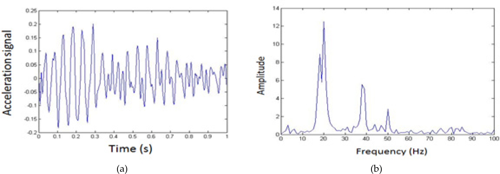
a) Acceleration time response, b) frequency spectrum.

Experimental and simulation modal analyses results are given in Table 5. There is no payload for the results given.

Table 5.

Experimental and simulation results.

Natural Frequency	Experiment (Hz)	Simulation (Hz)
f1	18.15	18.63
f2	20.54	22.53
f3	38.85	45.56

3.2 Case studies

Three cases are studied in this section. Each case has three different paths and the payload is 5 kg. The horizontal paths in Case-1, the vertical paths in Case-2 and the diagonal paths in Case-3 are considered as the tasks for the robot. The paths considered in these cases are shown in Fig 10.

Figure 10.

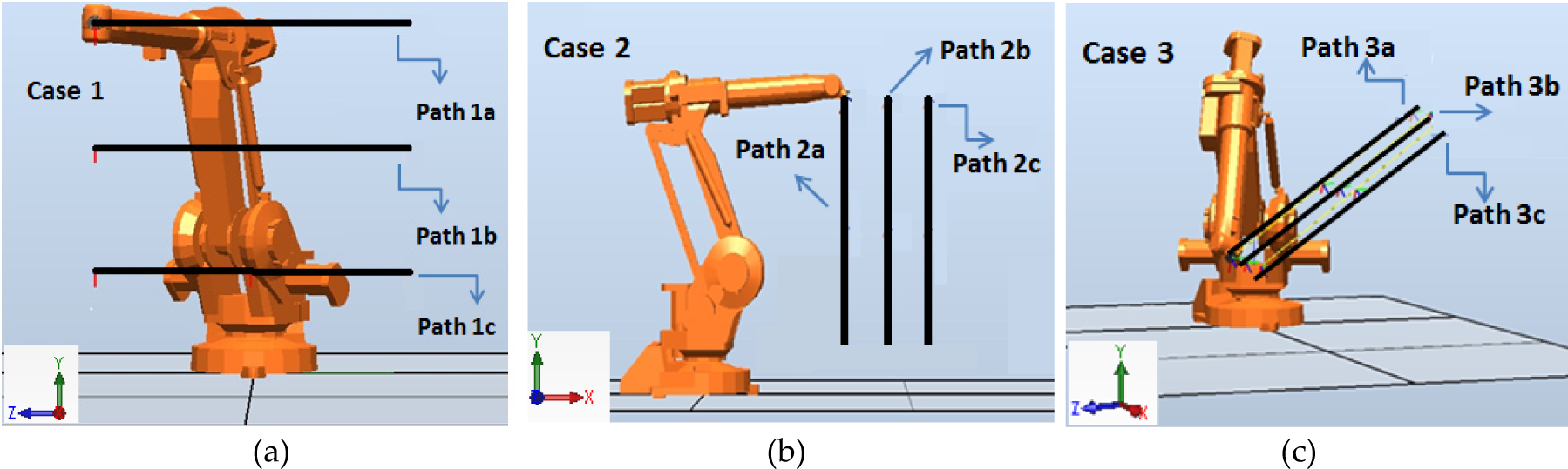
Different paths for the evaluation of the robot, a) Case-1, b) Case-2, c) Case-3.

The coordinates of the start points (S.P) and the end points (E.P) for the paths are given in Table 6.

Table 6.

Coordinates of the start and end points of the trajectories.

	Path-1a		Path-1b		Path-1c
	S.P.	E.P.	S.P.	E.P.	S.P.	E.P.
x	955	955	955	955	955	955
y	1195	1195	795	795	395	395
z	−500	500	−500	500	−500	500

	Path-2a		Path-2b		Path-2c
	S.P.	E.P.	S.P.	E.P.	S.P.	E.P.
x	700	700	900	900	1100	1100
y	150	1150	150	1150	150	1150
z	0	0	0	0	0	0

	Path-3a		Path-3b		Path-3c
	S.P.	E.P.	S.P.	E.P.	S.P.	E.P.
x	543.61	543.61	743.61	743.61	943.61	943.61
y	1000	400	1000	400	1000	400
z	400	−400	400	−400	400	−400

S.P.: Start Position, E.P.: End Position

In each case it is assumed that the end-point follows a line 1 metre long in 4 seconds. Acceptable paths are selected after the kinematic-kinetic-rigidity evaluations.

The robot passes the kinematic evaluation for all the cases as observed in Fig. 11. In Case-1, Path-1a is in the workspace and the motors do not exceed the velocity limits. The reaction forces are under the 50 % limit. The Motor-2 torque line is brown which indicates that it exceeds the 50 % limit. Umax also exceeds the 50 % limit. Path-1a is not recommended for the tasks which need high accuracy.

Figure 11.

Evaluation charts for different paths; Case-1 for (a) Path-1a, (b) Path-1b, (c) Path-1c, Case-2 for (d) Path-2a, (e) Path-2b, (f) Path-2c, Case-3 for (g) Path-3a, (h) Path-3b, (i) Path-3c.

All the parameters are in the green area for Path-1b. This path can be selected as the best one among the horizontal paths considering the strength of the robot. In this path, the payload can be increased or the task time can be decreased.

For Path-1c, Motor-2 torque exceeds the 50 % limit, but Umax is the smallest as compared with the previous paths. This path would be preferred if the application needed high precision and the maximum torque in Motor-2 could be decreased by increasing the task time.

Similar observations can be made for Case-2 and Case-3 paths. Motor-2 torque exceeds the 50 % limit for Path-2a and Path-2b and it exceeds the 100 % limit for Path-2c. It is preferred that all the parameters stay under the 50 % limit for a long life span. Therefore, the vertical path should be re-considered. The task time can be increased if it is not possible to change the path.

In Case 3, the Motor-2 torques for Path-3a and Path-3b are high. For Path-3c all the motor torques are under the 50 % limit, but Umax is high. Path-3c is not recommended for applications which need high precision.

In summary, the simulation results for the cases considered show that the motor torques in Case-2 are the highest. The robot is more rigid in Case-1 and the motor torques are in acceptable ranges. Path-3c in Case-3 has the lowest motor torques. Path-3c can be selected for pick and place applications. Path-1b can be considered for applications which need high precision.

4. Conclusions

Six axis robots are widely used in industry and they are manufactured by many companies. The manufacturers give the overall technical specifications such as the workspace, payload and maximum velocities. They also provide programs which evaluate the robot tasks considering the workspace only. In this work, it is offered that the task of a robot must be evaluated by kinematic, kinetic and rigidity analyses. A method for these analyses is introduced, which uses SolidWorks for modelling and assembly, CosmosMotion for the rigid body analysis and ABAQUS for the rigidity analysis. Integration software (IS) is developed in Visual BASIC for the easy and effective use of these programs. The results are given in the kinematic-kinetic-rigidity evaluation charts. Calculated motor velocities, bearing forces, motor torques, maximum end-point deflections, von Mises stresses and the first natural frequency are given as the percentages of the corresponding limit values. The percentage values are important for the life span of a robot. It is desired that all the percentages stay below a value typically 50 % for a given task. The same task can be performed by different approaches like the positioning of the work-piece with respect to the robot. The kinematic-kinetic-rigidity evaluation charts can be used to select the appropriate approach for a task.

Footnotes

5. Acknowledgements

The authors would like to acknowledge Dokuz Eylul University Research Fund (Project number: DPT-2003K120360) for its financial support of this work.

References

Stadler

, (1995), Analytical Robotics and Mechatronics, USA: McGraw-Hill.

Ghaudhary

Prasad

Sukavanum

(2012) Trajectory Tracking Control of Scorbot-Er V Plus Robot Manipulator Based on Kinematical Approach. International Journal of Engineering Science and Technology. Vol 4:1174–1182.

Lopes

Pires

Solteiro E. J.

(2011), Optimization of the Work piece Location in a Machining Robotic Cell. International Journal of Advanced Robotic Systems. j. Available: http://cdn.intechopen.com/pdfs/24608/InTechOptimization_of_the_workpiece_location_in_a_machining_robotic_cell.pdf Accessed 2011 May.

Albert

F.Y.C.

Koh

S. P.

Chen

C. P.

Tiong

S. K.

Edwin

S.Y.S.

(2011) Optimizing Joint Angels of Robotic Manipulator Using Genetic Algorithm. International Conference on Computer Engineering and Applications. Vol 2: 134–139.

Bobrow

J. E.

(1988) Optimal Robot Path Planning Using the Minimum-Time Criterion. Journal of Robotics and Automation. Vol 4: 443–450.

Yun

W-M

Y-G

(1996) Optimum Motion Planning in Joint Space for Robots Using Genetic Alghorithms. Robotics and Autonomous Systems. Vol 18: 373–393.

Karagulle

Malgaca

(2004), Analysis of End Point Vibrations of a Two-Link Manipulator by Integrated CAD/CAE Procedures. Finite Elements in Analysis and Design. Vol 40: 2049–2061.

Ata

A A

(2007), Optimal Trajectory Planning of Manipulators: A Review. Journal of Engineering Science and Technology. Vol 2: 32–54

Korayem

M. H.

Haghighi

Nikoobin

Alamdari

Korayem

A. H.

(2009) Determining Maximum Load Carrying Capacity of Flexible Link Manipulators. International Journal of Science and Technology. Vol 16: 440–450.

10.

Korayem

M. H.

Haghpanahi

Heidari

H. R.

(2010) Maximum Allowable Dynamic Load of Flexible Manipulators Undergoing Large Deformation. International Journal of Science and Technology. Vol 17: 61–74.

11.

Akdag

Karagulle

Malgaca

(2012) An Integrated Approach for Simulation of Mechatronic Systems Applied to a Hexapod Robot. Mathematics and Computers in Simulation. Vol 82: 818–835.

12.

Solidworks Premium Package-2007 (SolidWorks + CosmosMotion + CosmosWorks), Solidworks Corporation, www.solidworks.com (03.05.2012).

13.

SIMULIA, ABAQUS / CAE 6.9–1 (2009), http://www.3ds.com/products/simulia/portfolio/abaqus/overview/

14.

ABB IRB-1400, Industrial robot, http://www05.abb.com/global/scot/scot241.nsf/veritydisplay/e61508f4f3d8e993c125772e00558b68/$file/IRB%201410%20PR10325EN_R3.pdf

Kinematic-Kinetic-Rigidity Evaluation of a Six Axis Robot Performing a Task

Abstract

Keywords

1. Introduction

2. Integrated analysis

2.1 Flow chart of the analysis

2.2 Modelling of members and assembly of the robot

2.3. Integration software (IS)

2.3.1. Database for a planned task

2.3.2 Inverse kinematics and kinematic workspace evaluation in IS

2.3.3 Forward kinetics in IS

2.3.4 Finite element analysis for rigidity

3. Results and Discussions

3.1 Modal analysis

3.2 Case studies

4. Conclusions

Footnotes

5. Acknowledgements

References