Sage Journals: Discover world-class research

Abstract

The main goal of this manuscript is to present a simplification of the Euler-Lagrange methodology, which allows us to simplify the obtaining of dynamic model of a robot using the intrinsic properties of dynamic model, which allows to reduce the computation time when the model is programmed. Using the $L^{2}$ norm, the proposed methodology is compared with the Euler-Lagrange methodology for obtaining a performance index to determine the proposed simplification efficiency. The main contribution of this manuscript is to present a methodology to obtain the completely symmetric dynamic model.

Keywords

Methodology synthesized dynamic model performance index

1. Introduction

Obtaining the dynamic model of a robot manipulator plays an important role in the description of the system behavior for specific stimulus; this representation will allows us describing the system movement, analyzing diverse configurations of a manipulator and designing control structures [1 –4]. Describing the manipulator motion allows testing control strategies and motion planning techniques without the need to use a physically available system [5 –7]. The dynamic model analysis could be helpful for mechanical design of prototypes. Registering the forces and required torques to generate movement of the robot, provides information which serves to select drivers and actuators [6]. A robot manipulator is basically a positioning device. For controlling the position we must know the dynamic properties from the manipulator in order to know how much force has to be exerted on it causing the movement [1]. Minimum force and the manipulator will be slow to react. Maximum force and the arm may crash with an object or may oscillate about its desire position. Deriving the dynamic equation of motion for robots is not a simple task due to the large number of degrees of freedom and nonlinearities presented in the system [1 –7]. The main goal in this manuscript is presenting a comparison between two methods for obtaining the dynamic model of a robot manipulator in the joint space. The first method is based on the Euler-Lagrange formulation an the second one is a sintering of Euler-Lagrange's methodology by applying the model's properties.

This paper is organized as follows: Section 2 describes the simplified formulation and their main properties and assumptions; using both methodologies an evaluation example is presented in Section 3; In Section 4 we present a prototype description about the two degrees of freedom robot modeled on Section 3; the main experimental results are shown on Section 5 and the main computational results are shown on Section 6. Finally, we will offer some concluding remarks in Section 7.

2. Simplified methodology

The methodology proposed is based on the following simplification from Euler-Lagrange methodology:

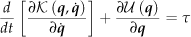
\frac{d}{d t} [\frac{\partial K (q, \dot{q})}{\partial \dot{q}}] + \frac{\partial U (q)}{\partial q} = τ

(1)

Basically, an operation and physical considerations are performed to simplify the original equation from Euler-Lagrange. The following are considerations which are made to simplify the Euler-Lagrange equation and get the proposal.

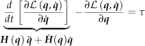
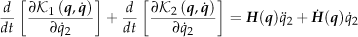
Analyzing Euler-Lagrange's equation, we can observe that the first term defines vectors H ( q ) q̈ + Ḣ(q)q̇ [1, 7 –9]:

\underset{H (q) \ddot{q} + \dot{H} (q) \dot{q}}{\underset{︸}{\frac{d}{d t} [\frac{\partial L (q, \dot{q})}{\partial \dot{q}}]}} - \frac{\partial L (q, \dot{q})}{\partial q} = τ

(2)

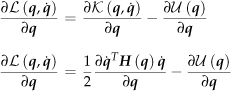
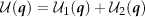
Proof. By replacing the lagrangian value $L (q, \dot{q})$ in the first term on Equation (2) we have:

\frac{d}{d t} [\frac{\partial L (q, \dot{q})}{\partial \dot{q}}] = \frac{d}{d t} [\frac{\partial K (q, \dot{q})}{\partial \dot{q}} - \frac{\partial U (q)}{\partial \dot{q}}]

(3)

we can observe that the potential energy U( q ) does not have dependent terms of q̇ ; thus when making the partial equation derivative (3), the potential energy is eliminated.

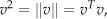
In classical mechanics, the kinetic energy is given by [6 –8]:

K (q, \dot{q}) = \frac{1}{2} m υ^{2} + \frac{1}{2} I {\dot{q}}^{2} = \frac{1}{2} {\dot{q}}^{T} H (q) \dot{q}

(5)

where m is the mass, v is the velocity of the body, I is the inertia force, q̇ is the joint velocity and H ( q ) is the symmetric positive definite manipulator inertial matrix. By substituting the Equation (5) in the Equation (4) and solving the operations we have:

\begin{array}{l} \frac{d}{d t} [\frac{\partial K (q, \dot{q})}{\partial \dot{q}}] = \frac{1}{2} \frac{d}{d t} [\frac{\partial {\dot{q}}^{T} H (q) \dot{q}}{\partial \dot{q}}] \\ \frac{d}{d t} [\frac{\partial K (q, \dot{q})}{\partial \dot{q}}] = H (q) \ddot{q} + \dot{H} (q) \dot{q} \end{array}

(6)

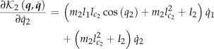
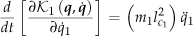
Now we proceed to analyze the second element from the Equation (2), which again replaces the Equation (5) as follows:

\begin{array}{l} \frac{\partial L (q, \dot{q})}{\partial q} = \frac{\partial K (q, \dot{q})}{\partial q} - \frac{\partial U (q)}{\partial q} \\ \frac{\partial L (q, \dot{q})}{\partial q} = \frac{1}{2} \frac{\partial {\dot{q}}^{T} H (q) \dot{q}}{\partial q} - \frac{\partial U (q)}{\partial q} \end{array}

(7)

If we replace the obtained results from equations (6) and (7) on Equation (2) and grouping respecting to q̇ we have:

\begin{array}{l} \underset{\frac{d}{d t} [\frac{\partial L (q, \dot{q})}{\partial \dot{q}}]}{\underset{︸}{H (q) \ddot{q} + \dot{H} (q) \dot{q}}} - \underset{\frac{\partial L (q, \dot{q})}{\partial q}}{\underset{︸}{\frac{1}{2} \frac{\partial {\dot{q}}^{T} H (q) \dot{q}}{\partial q} + \frac{\partial U (q)}{\partial q}}} = τ \\ H (q) \ddot{q} + (\dot{H} (q) - \frac{1}{2} \frac{\partial {\dot{q}}^{T} H (q)}{\partial q}) \dot{q} + \frac{\partial U (q)}{\partial q} = τ \end{array}

(8)

The Coriolis matrix C ( q, q̇ ) is defined as [1, 4, 7 –12]:

C (q, \dot{q}) = \dot{H} (q) - \frac{1}{2} \frac{\partial {\dot{q}}^{T} H (q)}{\partial q}

(9)

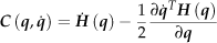
It is well-known that Coriolis matrix has the following properties [1, 4, 7 –12]:

Property 1. The following matrix:

{\dot{q}}^{T} [\dot{H} (q) - 2 C (q, \dot{q})] \dot{q} \equiv 0

(10)

it is skew-symmetric [1, 4, 7 –12].

Another important property related to the Coriolis matrix is [1, 4, 7 –12]:

\dot{H} (q) = C (q, \dot{q}) + C {(q, \dot{q})}^{T} .

(11)

Next, we present the set of assumptions underlying the methodology proposed.

Assumption 1. The transposed Coriolis matrix is defined as follow:

C {(q, \dot{q})}^{T} = \frac{1}{2} \frac{\partial {\dot{q}}^{T} H (q)}{\partial q}

(12)

Proof. Replacing Equation (11) in Equation (9) we have:

C (q, \dot{q}) = \underset{\dot{H} (q)}{\underset{︸}{C (q, \dot{q}) + C {(q, \dot{q})}^{T}}} - \frac{1}{2} \frac{\partial {\dot{q}}^{T} H (q)}{\partial q}

(13)

grouping the Equation (13) we have:

It is well known that generalized gravitational forces vector is defined as [1,4,7,8,11,12]:

g (q) = \frac{\partial U (q)}{\partial q}

(15)

Now, by substituting the Equation (11), (14) and (15) in the Equation (8) we have:

H (q) \ddot{q} + (C (q, \dot{q}) + C {(q, \dot{q})}^{T} - C {(q, \dot{q})}^{T}) \dot{q} + g (q) = τ

(16)

reducing terms:

we have:

H (q) \ddot{q} + C (q, \dot{q}) \dot{q} + g (q) = τ

(18)

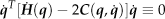
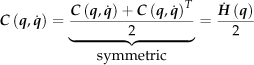
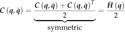
Until this moment the characteristics from Coriolis matrix and their interaction with the Euler-Lagrange equation have been described. It is necessary noting that the matrix C(q,q̇) can not be unique, but vector C (q,q̇)q̇ can. For this reason the goal of this manuscript proposing a Coriolis matrix structure.

Assumption 2. An interesting fact is that any square n × n matrix A can be represented as the sum of a symmetric matrix and a skew-symmetric matrix. This can be shown by the following decomposition:

A = \underset{s y m m e t r i c}{\underset{︸}{\frac{A + A^{T}}{2}}} + \underset{s k e w - s y m m e t r i c}{\underset{︸}{\frac{A - A^{T}}{2}}}

(19)

where the first term is symmetric and the second one is skew-symmetric [13].

Assumption 3. The symmetric part of the matrix A is considerably higher than the skew-symmetric part.

\underset{s y m m e t r i c}{\underset{︸}{\frac{A + A^{T}}{2}}} > > \underset{s k e w - s y m m e t r i c}{\underset{︸}{\frac{A - A^{T}}{2}}}

(20)

Assumption 4. If a square matrix B is expressed using

Assumption 2., subtracting the skew-symmetric matrices result in a symmetric term.

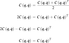
Proof. Expressing the matrix B agree with the Assumption 2. we have:

\underset{square - m a t r i x}{\underset{︸}{B}} = \underset{s y m m e t r i c}{\underset{︸}{\frac{B + B^{T}}{2}}} + \underset{s k e w - s y m m e t r i c}{\underset{︸}{\frac{B - B^{T}}{2}}}

(21)

the symmetrical term of the matrix B could be defined as:

\underset{s y m m e t r i c}{\underset{︸}{\frac{B + B^{T}}{2}}} = \underset{square - m a t r i x}{\underset{︸}{B}} - \underset{s k e w - s y m m e t r i c}{\underset{︸}{\frac{B - B^{T}}{2}}}

(22)

by grouping the equation we get:

\underset{grouping t e r m}{\underset{︸}{B - \frac{B - B^{T}}{2}}} = \frac{2 B - B + B^{T}}{2} = \underset{s y m m e t r i c}{\underset{︸}{\frac{B + B^{T}}{2}}}

(23)

as it is shown the result corresponds to the symmetric matrix B representation.

Assumption 5. Whereas the property described in Equation (11) and the Assumption 2., Assumption 3. and Assumption 4. we can define the Coriolis matrix based on the Ḣ ( q ) matrix as follow:

C (q, \dot{q}) = \underset{s y m m e t r i c}{\underset{︸}{\frac{C (q, \dot{q}) + C {(q, \dot{q})}^{T}}{2}}} = \frac{\dot{H} (q)}{2}

(24)

Proof. Expressing the Coriolis matrix according to the Assumption 2. we have:

C (q, \dot{q}) = \underset{s y m m e t r i c}{\underset{︸}{\frac{C (q, \dot{q}) + C {(q, \dot{q})}^{T}}{2}}} + \underset{s k e w - s y m m e t r i c}{\underset{︸}{\frac{C (q, \dot{q}) - C {(q, \dot{q})}^{T}}{2}}}

(25)

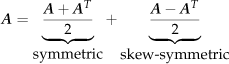
For the proposed methodology is considered only the symmetric part of the Equation (25) ignoring the effects of the skew-symmetric term Assumption 4., then we get:

C (q, \dot{q}) = \underset{s y m m e t r i c}{\underset{︸}{\frac{C (q, \dot{q}) + C {(q, \dot{q})}^{T}}{2}}}

(26)

It should be noted that the Equation (26) is valid under Assumption 3. because the influence of the skew-symmetric term is physically smaller.

Substituting Equation (11) into Equation (26) we get:

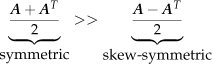
C (q, \dot{q}) = \underset{s y m m e t r i c}{\underset{︸}{\frac{C (q, \dot{q}) + C {(q, \dot{q})}^{T}}{2}}} = \frac{\dot{H} (q)}{2}

(27)

Considering the Assumption 2., Assumption 3. and Assumption 4. we can conclude that the most significant part of a square matrix is the symmetric part.

Assumption 6. According to the proposed methodology by ignoring the effects of skew-symmetric term, it is considered that the Coriolis matrix C ( q, q̇ ) is symmetric

C (q, \dot{q}) = C {(q, \dot{q})}^{T}

(28)

Proof. Solving the Coriolis matrix from the Equation (27) we have:

\begin{array}{l} C (q, \dot{q}) = \frac{C (q, \dot{q}) + C {(q, \dot{q})}^{T}}{2} \\ 2 C (q, \dot{q}) = C (q, \dot{q}) + C {(q, \dot{q})}^{T} \\ 2 C (q, \dot{q}) - C (q, \dot{q}) = C {(q, \dot{q})}^{T} \\ C (q, \dot{q}) = C {(q, \dot{q})}^{T} \end{array}

(29)

Assumption 7. Considering the Assumption 1., Equation (12), Assumption 5., Equation (24), and Assumption 6., Equation (28), we can perform following equality:

C (q, \dot{q}) = C {(q, \dot{q})}^{T} = \frac{1}{2} \frac{\partial {\dot{q}}^{T} H (q)}{\partial q} = \frac{\dot{H} (q)}{2}

(30)

In order to obtain the dynamic model of a robot manipulator based on the proposed methodology we proceed to implement the assumptions developed above. Substituting equations (15) and (30) in the Equation (8) we obtain:

\begin{array}{r} H (q) \ddot{q} + (\dot{H} (q) - \frac{1}{2} \frac{\partial {\dot{q}}^{T} H (q)}{\partial q}) \dot{q} + \frac{\partial U (q)}{\partial q} = τ \\ H (q) \ddot{q} + (\dot{H} (q) - \frac{1}{2} \dot{H} (q)) \dot{q} + g (q) = τ \\ H (q) \ddot{q} + \frac{1}{2} \dot{H} (q) \dot{q} + g (q) = τ \end{array}

(31)

Finally, applying Assumption 5., Equation (24), in Equation (31) we obtain the dynamic model of robot manipulator:

\begin{array}{l} H (q) \ddot{q} + \frac{1}{2} \dot{H} (q) \dot{q} + g (q) = τ \\ H (q) \ddot{q} + C (q, \dot{q}) \dot{q} + g (q) = τ \end{array}

(32)

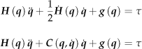
As it is shown in Equation (32) the Coriolis matrix is symmetric, generating a dynamic model completely symmetrical.

The simplified Euler-Lagrange's equation proposed in this methodology is defined as:

\frac{d}{d t} [\frac{\partial K (q, \dot{q})}{\partial \dot{q}}] + \frac{\partial U (q)}{\partial q} = τ

(33)

with the unique consideration for applying Assumption 5. to get the symmetrical representation of the dynamic model.

Finally we can conclude that the importance of developing alternative formulations for the dynamic model of a system is by obtaining tractable models for calculation systems more efficiently.

3. Example: Robot of two degrees of freedom

In order to understand the proposed formulation technique for obtaining the dynamic model, the proposed methodology is applied to a robot arm with two degrees of freedom.

3.1. Euler-Lagrange formulation

The first step consists of obtaining the forward kinematics of the system described in Figure 1; the forward kinematics are:

[\begin{matrix} x \\ y \end{matrix}] = [\begin{matrix} l_{1} \sin (q_{1}) + l_{2} \sin (q_{1} + q_{2}) \\ - l_{1} \cos (q_{1}) - l_{2} \cos (q_{1} + q_{2}) \end{matrix}] .

(34)

Figure 1.

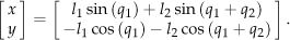
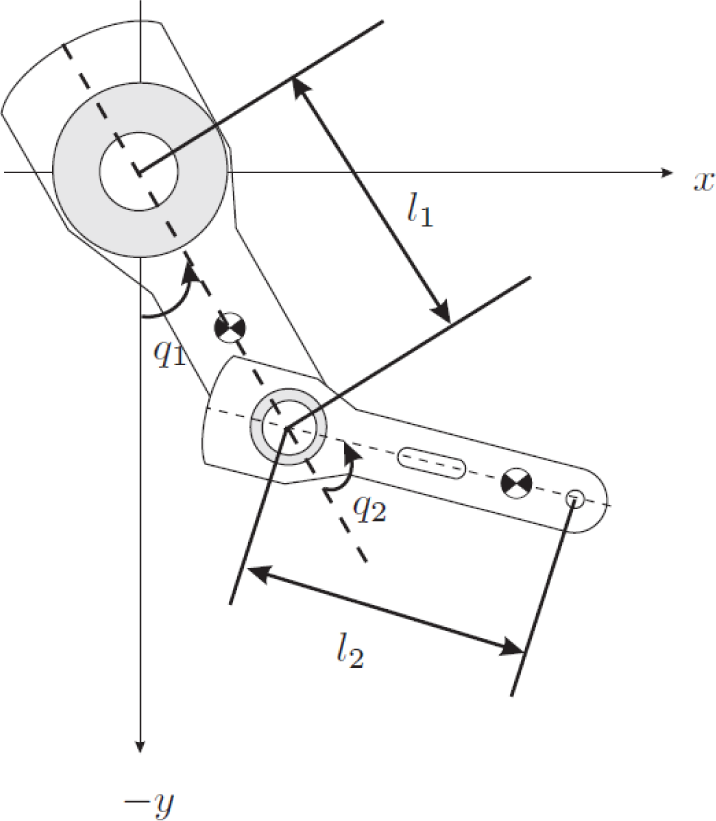
Robot of two degrees of freedom

Considering kinetic energy K ( q, q̇ ) of the system and the potential energy U( q ) we initiated the dynamic model calculation. We began to define kinetic energy K ( q, q̇ ) of the robot arm, which we can observe is under the influence of the joint velocity v [8]. The velocity v is the result to derive the position, which is described in vectorial form by the forward kinematics of the robot, Equation (34); thus we have derived the forward kinematics of a robot arm of two degrees of freedom is defined as [8]:

υ = [\begin{matrix} l_{1} \cos (q_{1}) + l_{c 2} \cos (q_{1} + q_{2}) l_{c 2} \cos (q_{1} + q_{2}) \\ l_{1} \sin (q_{1}) + l_{c 2} \sin (q_{1} + q_{2}) l_{c 2} \sin (q_{1} + q_{2}) \end{matrix}] [\begin{matrix} {\dot{q}}_{1} \\ {\dot{q}}_{2} \end{matrix}] .

(35)

By definition of the kinetic energy, Equation (5), the velocity is represented for the square; like the velocity v is a vector we must obtain the norm [8]:

υ^{2} = ‖ υ ‖ = υ^{T} υ,

(36)

thus we have:

υ_{1}^{2} = l_{c 1}^{2} {\dot{q}}_{1}^{2}

(37)

υ_{2}^{2} = l_{1}^{2} {\dot{q}}_{1}^{2} + l_{C 2}^{2} {({\dot{q}}_{1} + {\dot{q}}_{2})}^{2} + 2 l_{1} l_{C 2} \cos (q 2) ({\dot{q}}_{1}) ({\dot{q}}_{1} + {\dot{q}}_{2})

(38)

When replacing equations (37) and (38) in Equation (5) we have:

K_{1} (q, \dot{q}) = \frac{1}{2} (m_{1} l_{C 1}^{2} + I_{1}) {\dot{q}}_{1}^{2}

(39)

\begin{array}{c} K_{2} (q, \dot{q}) = \frac{1}{2} m_{2} l_{1}^{2} {\dot{q}}_{1}^{2} + m_{2} l_{1} l_{C 2} \cos (q_{2}) {\dot{q}}_{1} ({\dot{q}}_{1} + {\dot{q}}_{2}) \\ + \frac{1}{2} [m_{2} l_{C 2}^{2} + I_{2}] {({\dot{q}}_{1} | + {\dot{q}}_{2})}^{2} \end{array}

(40)

The total kinetic energy K( q, q̇ ) is defined as [8]:

K_{1} (q, \dot{q}) = K_{1} (q, \dot{q}) + K_{2} (q, \dot{q})

(41)

Now, we continue to find the potential energy U( q ):

U_{1} (q) = - m_{1} l_{C 1} g \cos (q_{1})

(42)

U_{2} (q) = - m_{1} l_{1} g \cos (q_{1}) - m_{2} l_{C 2} g \cos (q_{1} + q_{2})

(43)

the total potential energy U( q ) is defined as [8]:

U (q) = U_{1} (q) + U_{2} (q)

(44)

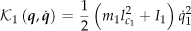
The next step is to calculate the Lagrangian $L (q, \dot{q})$ , which is defined as the difference between the total kinetic and total potential energy [8]:

L (q, \dot{q}) = K (q, \dot{q}) - U (q)

(45)

To calculate the Lagrangian we use equations (39), (40), (42) and (43) [8]:

\begin{array}{l} L (q, \dot{q}) = m_{2} l_{1} l_{C 2} \cos (q_{2}) {\dot{q}}_{1} ({\dot{q}}_{1} + {\dot{q}}_{2}) + m_{1} l_{C 1} g \cos (q_{1}) \\ + m_{2} l_{1} g \cos (q_{1}) + \frac{1}{2} (m_{1} l_{C 1}^{2} + m_{2} l_{1}^{2} + I_{1}) {\dot{q}}_{1}^{2} \\ + \frac{1}{2} [m_{2} l_{C 2}^{2} + I_{2}] {({\dot{q}}_{1} + {\dot{q}}_{2})}^{2} \\ + m_{2} l_{C 2} g \cos (q_{1} + q_{2}) \end{array}

(46)

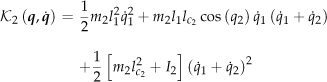
Now the next step is to evaluate the Euler-Lagrange Equation (2), by using the Lagrangian described in Equation (46) [8].

We initiate solving term $\frac{\partial L (q, \dot{q})}{\partial \dot{q}}$ ,

\begin{array}{l} \frac{\partial L (q, \dot{q})}{\partial {\dot{q}}_{1}} = 2 m_{2} l_{1} l_{C 2} \cos (q_{2}) {\dot{q}}_{1} + m_{2} l_{1} l_{C 2} \cos (q_{2}) {\dot{q}}_{2} \\ + m_{2} l_{c 2}^{2} {\dot{q}}_{2} + (m_{1} l_{c 1}^{2} + m_{2} l_{1}^{2} + m_{2} l_{C 2}^{2} + I_{1}) {\dot{q}}_{1} \\ + I_{2} {\dot{q}}_{1} + I_{2} {\dot{q}}_{2} \end{array}

(47)

\begin{array}{l} \frac{\partial L (q, \dot{q})}{\partial {\dot{q}}_{2}} = m_{2} l_{1} l_{C 2} \cos (q_{2}) {\dot{q}}_{1} + m_{2} l_{c 2}^{2} {\dot{q}}_{1} + I_{2} {\dot{q}}_{1} \\ + m_{2} l_{c 2}^{2} {\dot{q}}_{2} + I_{2} {\dot{q}}_{2} \end{array}

(48)

later the equations (47) and (48) are derived, then we have:

\begin{array}{l} \frac{d}{d t} [\frac{\partial L (q, \dot{q})}{\partial {\dot{q}}_{1}}] = 2 m_{2} l_{1} l_{C 2} \cos (q_{2}) {\ddot{q}}_{1} - 2 m_{2} l_{1} l_{C 2} \sin (q_{2}) {\dot{q}}_{1} {\dot{q}}_{2} \\ + m_{2} l_{1} l_{C 2} \cos (q_{2}) {\ddot{q}}_{2} - m_{2} l_{1} l_{C 2} \sin (q_{2}) {\dot{q}}_{2}^{2} \\ + m_{2} l_{c 2}^{2} {\ddot{q}}_{2} + (m_{1} l_{c 1}^{2} + m_{2} l_{1}^{2} + m_{2} l_{c 2}^{2} + I_{1}) {\ddot{q}}_{1} \\ + I_{2} {\ddot{q}}_{1} + I_{2} {\ddot{q}}_{2} \end{array}

(49)

\begin{array}{l} \frac{d}{d t} [\frac{\partial L (q, \dot{q})}{\partial {\dot{q}}_{2}}] = m_{2} l_{1} l_{C 2} \cos (q_{2}) {\ddot{q}}_{1} - m_{2} l_{1} l_{C 2} \sin (q_{2}) {\dot{q}}_{1} {\dot{q}}_{2} \\ + m_{2} l_{c 2}^{2} {\ddot{q}}_{1} + I_{2} {\ddot{q}}_{1} + m_{2} l_{c 2}^{2} {\ddot{q}}_{2} + I_{2} {\ddot{q}}_{2} \end{array}

(50)

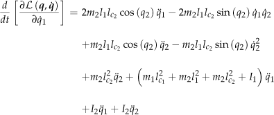
and finally we solve the term $\frac{\partial L (q, \dot{q})}{\partial \dot{q}}$ :

\begin{array}{l} \frac{\partial L (q, \dot{q})}{\partial q_{1}} = - m_{2} l_{C 2} g \sin (q_{1}) \cos (q_{2}) - m_{1} l_{C 1} g \sin (q_{1}) \\ - m_{2} l_{C 2} g \cos (q_{1}) \sin {(q)}_{2} - m_{2} l_{1} g \sin (q_{1}) \end{array}

(51)

\begin{array}{l} \frac{\partial L (q, \dot{q})}{\partial q_{2}} = - m_{2} l_{C 2} g \cos (q_{1}) \sin (q_{2}) - m_{2} l_{1} l_{C 2} \sin (q_{2}) {\dot{q}}_{1}^{2} \\ - m_{2} l_{C 2} g \sin (q_{1}) \cos (q_{2}) - m_{2} l_{1} l_{C 2} \sin (q_{2}) {\dot{q}}_{1} {\dot{q}}_{2} \end{array}

(52)

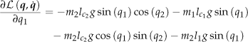
Grouping terms and applying trigonometrical identities we have:

\begin{array}{l} \frac{\partial L (q, \dot{q})}{\partial q_{1}} = - m_{1} l_{C 1} g \sin (q_{1}) - m_{2} l_{1} g \sin (q_{1}) \\ - m_{2} l_{C 2} g \sin (q_{1} + q_{2}) \end{array}

(53)

\begin{array}{l} \frac{\partial L (q, \dot{q})}{\partial q_{2}} = - m_{2} l_{1} l_{C 2} \sin (q_{2}) {\dot{q}}_{1}^{2} - m_{2} l_{1} l_{C 2} \sin (q_{2}) {\dot{q}}_{1} {\dot{q}}_{2} \\ - m_{2} l_{C 2} g \sin (q_{1} + q_{2}) \end{array}

(54)

thus we have:

\begin{array}{l} τ_{1} = [2 m_{2} l_{1} l_{C 2} \cos (q_{2}) + m_{1} l_{c 1}^{2} + m_{2} l_{1}^{2} + m_{2} l_{c 2}^{2}] {\ddot{q}}_{1} \\ + [I_{1} + I_{2}] {\ddot{q}}_{1} + [m_{2} l_{1} l_{C 2} \cos (q_{2}) + m_{2} l_{c 2}^{2} + I_{2}] {\ddot{q}}_{2} \\ - 2 m_{2} l_{1} l_{C 2} \sin (q_{2}) {\dot{q}}_{1} {\dot{q}}_{2} - m_{2} l_{1} l_{C 2} \sin (q_{2}) {\dot{q}}_{2}^{2} \\ + [m_{1} l_{C 1} + m_{2} l_{1}^{2}] g \sin (q_{1}) + m_{2} l_{C 2} g \sin (q_{1} + q_{2}) \end{array}

(55)

\begin{array}{l} τ_{2} = [m_{2} l_{1} l_{C 2} \cos (q_{2}) + m_{2} l_{c 2}^{2} + I_{2}] {\ddot{q}}_{1} + [m_{2} l_{c 2}^{2} + I_{2}] {\ddot{q}}_{2} \\ + m_{2} l_{1} l_{C 2} \sin (q_{2}) {\dot{q}}_{1}^{2} - m_{2} l_{1} l_{C 2} g \sin (q_{1} + q_{2}) \end{array}

(56)

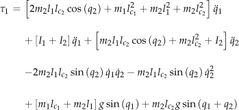
where τ₁ y τ₂ are the applied torque [8]. The vectorial representation of equations (55) and (56) are defined as follow:

[\begin{matrix} h_{11} & h_{12} \\ h_{21} & h_{22} \end{matrix}] [\begin{matrix} {\ddot{q}}_{1} \\ {\ddot{q}}_{2} \end{matrix}] + [\begin{matrix} c_{11} & c_{12} \\ c_{21} & c_{22} \end{matrix}] [\begin{matrix} {\dot{q}}_{1} \\ {\dot{q}}_{2} \end{matrix}] + [\begin{matrix} g_{1} \\ g_{2} \end{matrix}]

(57)

where:

\begin{array}{l} h_{11} = m_{1} l_{c 1}^{2} + m_{2} l_{1}^{2} + m_{2} l_{c 2}^{2} + 2 m_{2} l_{1} l_{c 2}^{} \cos (q_{2}) + I_{1} + I_{2} \\ h_{12} = m_{2} l_{c 2}^{2} + m_{2} l_{1} l_{c 2}^{} \cos (q_{2}) + I_{2} \\ h_{21} = m_{2} l_{c 2}^{2} + m_{2} l_{1} l_{c 2}^{} \cos (q_{2}) + I_{2} \\ h_{22} = m_{2} l_{c 2}^{2} + I_{2} \\ c_{11} = - 2_{m_{2}} l_{1} l_{c 2} \sin (q_{2}) {\dot{q}}_{2} \\ c_{12} = - m_{2} l_{1} l_{c 2} \sin (q_{2}) {\dot{q}}_{2} \\ c_{21} = m_{2} l_{1} l_{c 2} \sin (q_{2}) {\dot{q}}_{1} \\ c_{22} = 0 \\ g_{1} = (m_{1} l_{C 1} + m_{2} l_{1}) g \sin (q_{1}) + m_{2} g l_{C 2} \sin (q_{1} + q_{2}) \\ g_{2} = m_{2} g l_{C 2} \sin (q_{1} + q_{2}) \end{array}

(58)

3.2. Proposed methodology

In order to apply the proposed methodology based on the Equation (1), the first step consists by obtaining the forward kinematics of the system described in Figure 1; the forward kinematics are:

[\begin{matrix} x \\ y \end{matrix}] = [\begin{matrix} l_{1} \sin (q_{1}) + l_{2} \sin (q_{1} + q_{2}) \\ - l_{1} \cos (q_{1}) - l_{2} \cos (q_{1} + q_{2}) \end{matrix}] .

(59)

Considering kinetic energy K ( q, q̇ ) of the system, Equation (5), and the potential energy U( q ), we initiate the calculation of the dynamic model. We began to define kinetic energy K ( q, q̇ ) of the robot arm, which as we can observe is under the influence of the joint velocity v [8]. Velocity v is the result to derive the position, which is described in vectorial form by the forward kinematics of the robot, Equation (59); thus we have derived the forward kinematics of a robot arm of two degrees of freedom and is defined as:

υ = [\begin{matrix} l_{1} \cos (q_{1}) + l_{2} \cos (q_{1} + q_{2}) & l_{C 2} \cos (q_{1} + q_{2}) \\ l_{1} \sin (q_{1}) + l_{C 2} \sin (q_{1} + q_{2}) & l_{C 2} \sin (q_{1} + q_{2}) \end{matrix}] [\begin{matrix} {\dot{q}}_{1} \\ {\dot{q}}_{2} \end{matrix}] .

(60)

By definition of the kinetic energy, Equation (5), velocity is represented to the square; like velocity v is a vector we must obtain the norm:

υ^{2} = ‖ υ ‖ = υ^{T} υ,

(61)

thus we have:

υ_{1}^{2} = l_{c 1}^{2} q_{1}^{2}

(62)

υ_{2}^{2} = l_{1}^{2} {\dot{q}}_{1}^{2} + l_{c 2}^{2} {({\dot{q}}_{1} + {\dot{q}}_{2})}^{2} + 2 l_{1} l_{C 2} \cos (q_{2}) {\dot{q}}_{1} ({\dot{q}}_{1} + {\dot{q}}_{2})

(63)

When replacing Equation (52) in Equation (2) we have:

K_{1} (q, \dot{q}) = \frac{1}{2} (m_{1} l_{c 1}^{2} + I_{2}) {\dot{q}}_{1}^{2}

(64)

\begin{array}{l} K_{2} (q, \dot{q}) = \frac{1}{2} m_{2} l_{1}^{2} {\dot{q}}_{1}^{2} + m_{2} l_{1}^{} l_{C 2} \cos (q_{2}) {\dot{q}}_{1} ({\dot{q}}_{1} + {\dot{q}}_{2}) \\ + \frac{1}{2} [m_{2} l_{c 2}^{2} + I_{2}] {({\dot{q}}_{1} + {\dot{q}}_{2})}^{2} \end{array}

(65)

The total kinetic energy K( q, q̇ ) is defined as:

K (q, \dot{q}) = K_{1} (q, \dot{q}) + K_{2} (q, \dot{q})

(66)

Now, we continue to finding the potential energy U( q ), thus we have:

U_{1} (q) = - m_{1} l_{C 1} g \cos (q_{1})

(67)

U_{2} (q) = - m_{2} l_{1} g \cos (q_{1}) - m_{2} l_{C 2} g \cos (q_{1} + q_{2})

(68)

the total potential energy is defined as:

U (q) = U_{1} (q) + U_{2} (q)

(69)

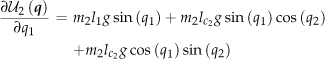
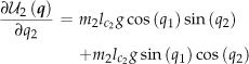
Now we solve Equation (6) by parts, the first part is the term $\frac{\partial L (q, \dot{q})}{\partial \dot{q}}$ :

\frac{\partial K_{1} (q, \dot{q})}{\partial {\dot{q}}_{1}} = (m_{1} l_{c 1}^{2} + I_{1}) {\dot{q}}_{1}

(70)

\frac{\partial K_{1} (q, \dot{q})}{\partial {\dot{q}}_{2}} = 0

(71)

\begin{array}{l} \frac{\partial K_{2} (q, \dot{q})}{\partial {\dot{q}}_{1}} = (m_{2} l_{1}^{2} + m_{2} l_{C 2}^{2} + 2 m_{2} l_{1} l_{C 2} \cos (q_{2}) + I_{2}) {\dot{q}}_{1} \\ + (m_{2} l_{1} l_{C 2} \cos (q_{2}) + m_{2} l_{C 2}^{2} + I_{2}) {\dot{q}}_{2} \end{array}

(72)

\begin{array}{l} \frac{\partial K_{2} (q, \dot{q})}{\partial {\dot{q}}_{2}} = (m_{2} l_{1} l_{C 2} \cos (q_{2}) + m_{2} l_{C 2}^{2} + I_{2}) {\dot{q}}_{1} \\ + (m_{2} l_{C 2}^{2} + I_{2}) {\dot{q}}_{2} \end{array}

(73)

the following step is to derive equations (70)–(73):

\frac{d}{d t} [\frac{\partial K_{1} (q, \dot{q})}{\partial {\dot{q}}_{1}}] = (m_{1} l_{C 1}^{2}) {\ddot{q}}_{1}

(74)

\frac{d}{d t} [\frac{\partial K_{1} (q, \dot{q})}{\partial {\dot{q}}_{2}}] = 0

(75)

\begin{array}{l} \frac{d}{d t} [\frac{\partial K_{2} (q, \dot{q})}{\partial {\dot{q}}_{1}}] = (m_{2} l_{1}^{2} + m_{2} l_{C 2}^{2} + 2 m_{2} l_{1} l_{C 2} \cos (q_{2})) {\ddot{q}}_{1} \\ + (m_{2} l_{1} l_{C 2} \cos (q_{2}) + m_{2} l_{C 2}^{2} + I_{2}) {\ddot{q}}_{2} \\ + (I_{1} + I_{2}) {\ddot{q}}_{2} - 2 m_{2} l_{1} l_{C 2} \sin (q_{2}) {\dot{q}}_{1} {\dot{q}}_{2} \\ - m_{2} l_{1} l_{C 2} \sin (q_{2}) {\dot{q}}_{1} {\dot{q}}_{2} \end{array}

(76)

\begin{array}{l} \frac{d}{d t} [\frac{\partial K_{2} (q, \dot{q})}{\partial {\dot{q}}_{2}}] = (m_{2} l_{1} l_{C 2} \cos (q_{2}) + m_{2} l_{C 2}^{2}) {\ddot{q}}_{1} \\ + (m_{2} l_{C 2}^{2}) {\ddot{q}}_{2} - m_{2} l_{1} l_{C 2} \sin (q_{2}) {\dot{q}}_{1} {\dot{q}}_{2} \\ + I_{2} {\ddot{q}}_{1} + I_{2} {\ddot{q}}_{2} \end{array}

(77)

accommodating equations (74)–(77):

\frac{d}{d t} [\frac{\partial K_{1} (q, \dot{q})}{\partial {\dot{q}}_{2}}] + \frac{d}{d t} [\frac{\partial K_{2} (q, \dot{q})}{\partial {\dot{q}}_{1}}] = H (q) {\ddot{q}}_{1} + \dot{H} (q) {\dot{q}}_{1}

(78)

\frac{d}{d t} [\frac{\partial K_{1} (q, \dot{q})}{\partial {\dot{q}}_{2}}] + \frac{d}{d t} [\frac{\partial K_{2} (q, \dot{q})}{\partial {\dot{q}}_{2}}] = H (q) {\ddot{q}}_{2} + \dot{H} (q) {\dot{q}}_{2}

(79)

Considering only the elements which form the vector H(q)q̈ we have:

\begin{array}{l} H (q) {\ddot{q}}_{1} = (m_{1} l_{C 1}^{2} + m_{2} l_{C 2}^{2} + m_{2} l_{1}^{2} + I_{1} + I_{2}) {\ddot{q}}_{1} \\ + (m_{2} l_{1} l_{C 2} \cos (q_{2}) + m_{2} l_{C 2}^{2} + I_{2}) {\ddot{q}}_{2} \\ + 2 m_{2} l_{1} l_{C 2} \cos (q_{2}) {\ddot{q}}_{1} \end{array}

(80)

\begin{array}{l} H (q) {\ddot{q}}_{2} = (m_{2} l_{1} l_{C 2} \cos (q_{2}) + m_{2} l_{C 2}^{2} + I_{2}) {\ddot{q}}_{1} \\ + (m_{2} l_{C 2}^{2} + I_{2}) {\ddot{q}}_{2} \end{array}

(81)

The vectorial representation of equations (80) and (81) are described by:

H (q) \ddot{q} = [\begin{matrix} h_{11} & h_{12} \\ h_{21} & h_{22} \end{matrix}] [\begin{matrix} {\ddot{q}}_{1} \\ {\ddot{q}}_{2} \end{matrix}]

(82)

where:

h_{11} = m_{1} l_{C 1}^{2} + m_{2} l_{1}^{2} + m_{2} l_{C 2}^{2} + 2 m_{2} l_{1} l_{C 2} \cos (q_{2}) + I_{1} + I_{2}

(83)

h_{12} = m_{2} l_{C 2}^{2} + m_{2} l_{1} l_{C 2} \cos (q_{2}) + I_{2}

(84)

h_{21} = m_{2} l_{C 2}^{2} + m_{2} l_{1} l_{C 2} \cos (q_{2}) + I_{2}

(85)

h_{22} = m_{2} l_{C 2}^{2} + I_{2}

(86)

When comparing equations (58) and (83) these are observed that the same value of the inertial matrix H ( q ) has been obtained. Now, considering only the part of the equations (74)–(77) which form the vector Ḣ(q)q̇ we have:

{\dot{h}}_{11} = - 2 m_{2} l_{1} l_{C 2} \sin (q_{2}) {\dot{q}}_{2}

(87)

{\dot{h}}_{12} = - m_{2} l_{1} l_{C 2} \sin (q_{2}) {\dot{q}}_{2}

(88)

{\dot{h}}_{21} = - m_{2} l_{1} l_{C 2} \sin (q_{2}) {\dot{q}}_{2}

(89)

{\dot{h}}_{22} = 0

(90)

In order to obtain the Coriolis matrix, the equality described on the Assumption 5. Equation (24) will be evaluated:

c_{11} = \frac{{\dot{h}}_{11}}{2} = - m_{2} l_{1} l_{C 2} \sin (q_{2}) {\dot{q}}_{2}

(91)

c_{12} = \frac{{\dot{h}}_{12}}{2} = - \frac{m_{2} l_{1} l_{C 2} \sin (q_{2}) {\dot{q}}_{2}}{2}

(92)

c_{21} = \frac{{\dot{h}}_{21}}{2} = - \frac{m_{2} l_{1} l_{C 2} \sin (q_{2}) {\dot{q}}_{2}}{2}

(93)

c_{22} = \frac{{\dot{h}}_{22}}{2} = 0

(94)

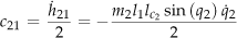
The vectorial representation of equations (91)–(94) are:

c (q, \dot{q}) \dot{q} = [\begin{matrix} c_{11} & c_{12} \\ c_{21} & c_{22} \end{matrix}] [\begin{matrix} {\dot{q}}_{1} \\ {\dot{q}}_{2} \end{matrix}]

(95)

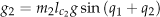
As the matrix of Centripetal and Coriolis torques is observed, it is symmetrical, being this value the suitable one for the system. Finally, we calculate the gravitational torque by applying the Equation (15):

\frac{\partial U_{1} (q)}{\partial q_{1}} = m_{1} l_{C 1} g \sin (q_{1})

(96)

\frac{\partial U_{1} (q)}{\partial q_{2}} = 0

(97)

\begin{array}{l} \frac{\partial U_{2} (q)}{\partial q_{1}} = m_{2} l_{1} g \sin (q_{1}) + m_{2} l_{C 2} g \sin (q_{1}) \cos (q_{2}) \\ + m_{2} l_{C 2} g \cos (q_{1}) \sin (q_{2}) \end{array}

(98)

\begin{array}{l} \frac{\partial U_{2} (q)}{\partial q_{2}} = m_{2} l_{C 2} g \cos (q_{1}) + \sin (q_{2}) \\ + m_{2} l_{C 2} g \sin (q_{1}) \cos (q_{2}) \end{array}

(99)

accommodating equations (96)–(99):

g_{1} = \frac{\partial U_{1} (q)}{\partial q_{1}} + \frac{\partial U_{2} (q)}{\partial q_{1}}

(100)

g_{2} = \frac{\partial U_{1} (q)}{\partial q_{2}} + \frac{\partial U_{2} (q)}{\partial q_{2}}

(101)

thus we have:

g_{1} = (m_{1} l_{C 1} + m_{2} l_{1}) g \sin (q_{1}) + m_{2} l_{C 2} g \sin (q_{1} + q_{2})

(102)

g_{2} = m_{2} l_{C 2} g \sin (q_{1} + q_{2})

(103)

Finally, if you want to get the same representation of Coriolis matrix obtained by applying the Euler-Lagrange method it will be used any of the following matrices:

C (q, \dot{q}) = \dot{H} (q) + [\begin{matrix} 0 & 0 \\ c_{21} . ({\dot{q}}_{1} + {\dot{q}}_{2}) & 0 \end{matrix}]

(104)

C (q, \dot{q}) = 2 C (q, \dot{q}) + [\begin{matrix} 0 & 0 \\ c_{21} . ({\dot{q}}_{1} + {\dot{q}}_{2}) & 0 \end{matrix}]

(105)

4. Experimental system description

In this section we'll describe the prototype used to evaluate the dynamic models obtained by using both methodologies. In general terms, it consists in a hardware part and friendly software for its operation. Direct drive vertical robot manipulator with two degrees of freedom had rigid link with revolute joints. It is equipped with two brushless direct drive servo actuators from Compumotor® used to drive the joints without gear reductions. Advantages of this type of direct drive actuators includes freedom from backslash and significantly lower joint friction compared to actuators with gear drives. Motors used in the robot are listed in Table 1. The servos are operated in torque mode, so motors act like a source torque and they accept an analog voltage as a reference of signal torque [14].

Table 1.

Servo actuators of the experimental robot

Link	Model	Torque N/m	p/rev
Shoulder	DM1200A	200	1,024,000
Elbow	DM1015B	15	1,024,000

The position of information is obtained from incremental encoders located in the motors. The standard backwards make difference with algorithm applied to the joint positions measurements which were used to generate the velocity signals. The links were made of 6,061 aluminum; the manipulator workspace is a circle with 0.98 meter of radius. DS1102 motion control board manufactured by dSpace® based on the Texas Instrument TMS320C3DSP is used for execution of control algorithm. The sampling period is actually set at 2.5 ms [14]. The physical parameters of the system are described in Table 2 [8,14].

Table 2.

Physical parameters of the prototype

Description	Notation	Value Units
Link 1	l ₁	0.4500 m
Link 2	l ₂	0.4500 m
Center of mass 1	l _c1	0.0910 m
Center of mass 2	l _c2	0.0480 m
Mass of the link 1	m ₁	23.902 Kg
Mass of the link 2	m ₂	3.8800 Kg
Moment of inertia 1	I ₁	1.2660 Kg m²
Moment of inertia 2	I ₂	0.0930 Kg m²
Gravity	g	9.8100 m/s2

The next step is to evaluate both models using the physical parameters of the robot arm with two degrees of freedom, Table 2, later compare through simulations performed with the program SIMNON® [14].

4.1. Dynamic model using Euler-Lagrange formulation

Considering the matrix representation of the dynamic model, Equation (57), and the physical parameters of the prototype [8], Table 2, we have:

h_{11} = 2 .3515719820+ 0 .167616000cos(q_{2})

(106)

h_{12} = 0 .1019395200+ 0 .083808000cos(q_{2})

(107)

h_{21} = 0 .1019395200+ 0 .083808000cos(q_{2})

(108)

h_{22} = 0 .1019395200

(109)

c_{11} = -0 .167616000sin(q_{2}) {\dot{q}}_{2}

(110)

c_{12} = -0 .083808000sin(q_{2}) {\dot{q}}_{2}

(111)

c_{21} = +0 .083808000sin(q_{2}) {\dot{q}}_{1}

(112)

c_{22} = 0

(113)

g_{1} = 38 .46581442sin(q1) + 1 .827014400sin(q_{1} + q_{2})

(114)

g_{2} = 1 .827014400sin(q_{1} + q_{2})

(115)

4.2. Dynamic model using the simplified methodology

Using the physical parameters of the prototype described in the Table 2 we can evaluate the equations (83)–(86), (91)–(94) and (102)–(103) and getting the dynamic model based on the Simplified methodology.

h_{11} = 2 .3515719820+ 0 .167616000cos(q_{2})

(116)

h_{12} = 0 .1019395200+ 0 .083808000cos(q_{2})

(117)

h_{21} = 0 .1019395200+ 0 .083808000cos(q_{2})

(118)

h_{22} = 0 .1019395200

(119)

c_{11} = -0 .08380800000sin(q_{2}) {\dot{q}}_{2}

(120)

c_{12} = -0 .04190400000sin(q_{2}) {\dot{q}}_{2}

(121)

c_{21} = -0 .04190400000sin(q_{2}) {\dot{q}}_{2}

(122)

c_{22} = 0

(123)

g_{1} = 38 .46581442sin(q_{1}) + 1 .827014400sin(q_{1} + q_{2})

(124)

g_{2} = 1 .827014400sin(q_{1} + q_{2})

(125)

5. Experimental results

In order to support our theoretical developments in this section we present an experimental result using the proposed methodology for evaluating a robot manipulator of two degrees of freedom.

In order to evaluate the behavior from the obtained models we must program a PD control structure, to make a simulation using SIMNON® then an experiment with the physical prototype everything, with the objective to compare the behavior obtained by means from the performance index using the $L^{2}$ norm [14]. The experiment consist on moving the manipulator's end-effector from its initial position q to a desired position q_d. We have made the following experiment using the desired position q _d described in the following way:

[\begin{matrix} q_{d 1} \\ q_{d 2} \end{matrix}] = [\begin{matrix} \frac{π}{4} \\ \frac{π}{2} \end{matrix}] = [\begin{matrix} 0.7854 \\ 1.5708 \end{matrix}]

(126)

where q_d1 and q_d2 represent the desired position vector. The initial positions and velocities were set to zero (for example a home position). The evaluated controllers have been written in C language. The sampling rate was executed at 2.5 ms [14]. The value from gains used in the tuning of the PD control structure are listed in the following table:

Table 3.

Gains used in the experiment

K _p1	64.72
K _v1	48.54
K _p2	32.36
K _v2	6.472

An important observation needs to be done: it is the value from gains used in the simulator should be the same as those programmed in the physical system. This ensures that by plotting the behavior of the simulations and data from the real system are in the same conditions.

Figure 3 shows the responses generated simultaneously by using the Euler-Lagrange methodology [E-L], the proposed methodology [P-M] and readings from the sensors of the robot. Specifically shows the response of the first link. Apparently the behavior is the same, but as shown in Figure 4 making a zoom around (1.070–1.115), there is a difference between the methods of simulation and current system behavior. As shown in Figure 4 the proposed methodology is better because it follows the robot behavior. Performing a graphs comparison shows a slight variation between which represents the absence of the skew-symmetric part of the Coriolis matrix [1, 8, 14]. The friction phenomena were not modeled for compensation purpose. Nevertheless, in spite of the presence of the friction, phenomenon which doesn't have a mathematical structure can't be modeled [8, 14].

Figure 2.

Direct-Drive robot arm of two degrees of freedom

Figure 3.

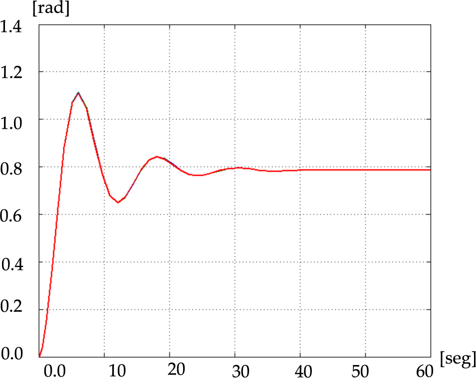
First joint behavior (Robot and both metodologies)

Figure 4.

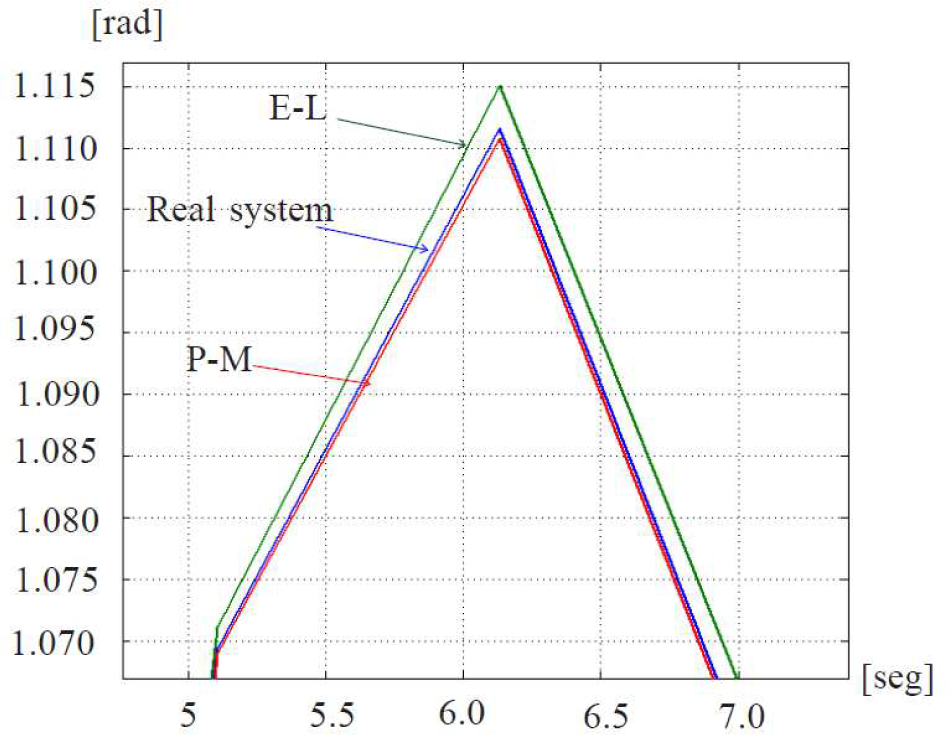
Specic area of comparison of the behavior

5.1. Performance Index

Robot manipulators are very complex mechanical system, due to the nonlinear and multivariable nature of its dynamic behavior. For this reason, in the robotics community it is not well established a criteria for an appropriate evaluation in controllers for robots [1,14].

However, it is accepted in practice to compare the performance of controllers by using the scalar-valued $L^{2}$ norm as an objective numerical measure for an entire error curve [14]. The $L^{2} [\tilde{q}]$ norm measures the root-mean-square average of the q˜ position error, which is given by:

L^{2} [\tilde{q}] = \sqrt{\frac{1}{t - t_{0}} \int_{t_{0}}^{t} {‖ \tilde{q} ‖}^{2} d t}

(127)

where t₀, t ∈ ℝ₊ are the initial and final times, respectively. A $L^{2} [\tilde{q}]$ smaller represents a less error position and it indicates the best performance for the evaluated controller [14]. The overall results are summarized in Figure 5 which includes the performance indexes for the analyzed controllers. For averaging stochastic influences, the data presentation in this figure represents the mean about root-mean-square error position vector norm of ten runs [14].

Figure 5.

Performance index

6. Computation time

After analyzing the performance index of both methods it is important to compare the computation time to determine the best performance. By considering several elementary systems we will demonstrate that the reason for the emergence of quite complex behavior is feedback. In a system model embodying feedback loops, state variables are fed back to influence their own rates of change. Feeding back a state variable to its own derivative can be direct or also involve several other state variables. Qualitative analysis of the feedback loops in a system can give insights into its possible behaviors. Most important is whether a feedback loop is positive or negative. When traversing thee feedback loop, we can count the signs of the direct influences between the state variable. When the sign of a function f_i is positive, we speak of a positive influence from q_i–1 to q_i, which means that a positive value of q_i-1 will make q_i increase [15].

In order to analyze the performance we analyze the computation time that takes each algorithm to solve an operation. The computation time evaluation is performed using Matlab© symbolic algorithms. To set the symbolic algorithm for obtaining the dynamic model based on Euler-Lagrange methodology is used in the following equation:

\frac{d}{d t} [\frac{\partial L (q, \dot{q})}{\partial \dot{q}}] - \frac{\partial L (q, \dot{q})}{\partial q} = τ

(128)

The symbolic program programmed in 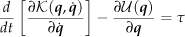Matlab© shows that the Euler-Lagrange methodology use 2.9124e + 001 seconds to perform an operation. While the proposed method to obtain the dynamic model is based on the following equation:

\frac{d}{d t} [\frac{\partial K (q, \dot{q})}{\partial \dot{q}}] - \frac{\partial U (q)}{\partial q} = τ

(129)

performing an operation within 2.1618e + 001 seconds.

The simulation of dynamic models, obtained using both methods were compared with experimental data and applying the $L^{2}$ norm was obtained performance index, which is presented in Figure 6.

Figure 6.

Computation time

The models are evaluated solving them for the same position, using the same gains and the same numerical method (Runge-Kutta 4). The computation time was obtained using Matlab©.

Should be noted that if in performing the task of moving the system to only one position there is a difference in time of execution, it is cumulative, so that, when performing a task consisting of a sequence of desired positions, using the proposed methodology, the model will make the task much faster compared with the model obtained using Euler-Lagrange methodology.

7. Conclusions

It is noteworthy that a model is an abstraction of reality used to address a problem, usually is simplified in symbolic terms and posed from a mathematical point of view.

To model it is necessary to raise a number of hypotheses, so that the system is represented and sufficiently defined in the idealization, but also seeks to keep the simple model enough to be manipulated and studied [15, 16].

Obtaining the mathematical model implies a number of assumptions, simplifications and limitations that involves tolerable errors. This means that there is always uncertainty when the system is modeled and it is reasonable to know that some extent these involved errors. Often the model contains errors due to the complexity of the system, the unknown parameters and external shocks are difficult to quantify [15, 16].

These errors can be disastrous in practice therefore continually are developed new methods and control laws that seek to be robust for uncertainties in the model. Although various methods have been developed for obtaining the dynamic model of a system, it is still inaccurate, introducing tolerable errors ultimately affects system performance [15, 16].

The methodology proposed in this manuscript presents a better performance than the traditional methodology of Euler-Lagrange, because as it is observed it presents one better structure of the matrix of Centripetal and Coriolis torques, fulfilling the proposed theorems and the properties of the model. This allows us to conclude that from the mathematical point of view the simplified methodology is easier to manipulate than the methodology of Euler-Lagrange, in addition the synthesized method presents a better performance.

It is necessary to emphasize that the proposed method is the result of the rigorous studies of the traditional method from Euler-Lagrange, being validated the procedures when fulfilling the properties of the dynamic model, which gives the mathematical formality and its validity.

Footnotes

8. Acknowledgements

The authors thanks the support received by Facultad de Ciencias de la Electrónica on Benemérita Universidad Autónoma de Puebla, Mexico; and also by the revision on manuscript to Lic. Oscar R. Quirarte Castellanos.

References

Spong

Mark W.

Lewis

F. L.

and Abdallah

C. T.

, Robot Control. Dynamics, Motion Planning, and Analysis, (New York, IEEE Press, 1993).

Lee

C. S. G.

González

R. C.

and Fu

K. S.

, Tutorial on Robotics, 2nd Edition (Silver Springs, MD: IEEE Computer Society Press, 1986).

Brady

Hollerbach

J. H.

Jhonson

T. L.

Lozano-Pérez

, and Mason

M. T.

Robot Motion: Planning and Control, (Cambridge, MA: MIT Press, 1982).

Critchlow

A. J.

, Introduction to Robotics, (New York, Macmillan, 1985).

Bejczy

A. K.

, Robot arm dynamics and control, Technical Memo 33–669, Pasadena, CA: NASA Jet Propulsion Laboratory, 1974.

Beni

and Hackwood

, Eds. Recent Advances in Robotics, (New York: John Wiley and sons, 1985).

Spong

M. W.

and Vidyasagar

, Robot dynamics and control, (New York: John Wiley and sons, 1989).

Kelly

Rafael

and Santibáñez

Victor

, Control de Movimiento de Robots Manipuladores, (Madrid: Prentice Hall, 2003)

Astolfi

Alessandro

and Marconi

Lorenzo

, Analysis and Design of Nonlinear Control Systems: In Honor of Alberto Isidori, (Springer; Softcover reprint of hardcover 1st ed. 2008), 2010

10.

Isidori

Alberto

, Nonlinear Control Systems (Communications and Control Engineering), (Springer; 3rd edition, 1995).

11.

Sciavicco

and Siciliano

, Modeling and control of robot manipulators, (New York: McGraw Hill, 1996).

12.

Craig

J. J.

, Introduction to Robotics, mechanics and control, (New York: Addison-Wesley, 1986).

13.

Kreyszig

Erwin

, Advanced Engineering Mathematics, (New York, Wiley International Edition, 2006).

14.

Sánchez-Sánchez

and Reyes-Cortés

, “A Polynomial Family of PD-Type Cartesian Controller”, International Journal of Robotics and Automation, 23(2), pp. 79–87, 2008.

15.

Zeigler

Bernard P.

Praehofer

Herbert

and Kim

Tang Gon

, Theory of modeling and Simulation, Integrating Discrete Events and Continuous Complex Dyamic Systems,(USA, Elsevier Science, 1976).

16.

Siciliano

Bruno

and Villani

Luigi

, Robot Force Control,(Klumer Academic Publishers, 1999).

Simplied Methodology for Obtaining the Dynamic Model of Robot Manipulators

Abstract

Keywords

1. Introduction

2. Simplified methodology

3. Example: Robot of two degrees of freedom

3.1. Euler-Lagrange formulation

3.2. Proposed methodology

4. Experimental system description

4.1. Dynamic model using Euler-Lagrange formulation

4.2. Dynamic model using the simplified methodology

5. Experimental results

5.1. Performance Index

6. Computation time

7. Conclusions

Footnotes

8. Acknowledgements

References