Sage Journals: Discover world-class research

Abstract

In this paper, a novel forward adaptive neural MIMO NARX model is used for modelling and identifying the forward kinematics of an industrial 3-DOF robot arm system. The nonlinear features of the forward kinematics of the industrial robot arm drive are thoroughly modelled based on the forward adaptive neural NARX model-based identification process using experimental input-output training data. This paper proposes a novel use of a back propagation (BP) algorithm to generate the forward neural MIMO NARX (FNMN) model for the forward kinematics of the industrial 3-DOF robot arm. The results show that the proposed adaptive neural NARX model trained by a Back Propagation learning algorithm yields outstanding performance and perfect accuracy.

Keywords

Forward Kinematics of an Industrial 3-DOF Robot Arm Back Propagation Learning Algorithm (BP)Adaptive Neural MIMO NARX Model Modelling and Identification

1. Introduction

The robot control problems can be divided into two main areas: kinematics control (the coordination of the links of a kinematics chain to produce the desired motion of the robot) and dynamic control (the driving of the actuator of a mechanism to follow the commanded positional velocities). In general, the control strategies used in robots involve position coordination in a Cartesian space by direct or indirect kinematics methods. Forward kinematics comprises the computation needed to find the join angles for a given Cartesian position and the orientation of the end effectors. This computation is fundamental to the control of robot arms but it is very difficult to calculate a forward kinematics solution of the robot arm. For this solution, most industrial robot arms are designed using a nonlinear algebraic computation for finding the forward kinematics solution. It is well known in literature that there is no unique solution for forward kinematics. This is the reason why it is important to apply artificial neural network models to obtain a solution.

Novel approaches of artificial neural network (ANN) models have been proposed to control the motion of robot arms. In these works, two types of ANN models are used. The first kind of ANN model is the MLP (multilayer perceptron), which is popular as a back propagation neural model. In this network, gradient descent types of learning rules are applied. The second kind of ANN model is the PPN (polynomial poly-processor neural network), where a polynomial equation was used. Here, work has been undertaken to find the best ANN configuration for the problem. It was found that between MLP and PPN, MLP gives better results as compared with PPN, considering the average percentage error as the performance index.

Alavandar and Nigam [1] developed a Neuro-Fuzzy-based approach for a forward kinematics solution for industrial robot arms. In their paper, it is shown that by using the ability of an Adaptive Neuro-Fuzzy Inference System (ANFIS) to learn from training data, it is possible to create an implementation of a representative fuzzy inference system using a BP neural network-like structure, with limited mathematical representation of the system. Computer simulations conducted on 2-DOF and 3-DOF robot arms showed the effectiveness of the approach.

Morris et al. [2] developed an artificial neural network for finding the kinematics of a robot arm using a look-up table. The neural networks utilized were multi-layered perceptrons with a back-propagation training algorithm. They used 5 hidden layer neurons with the rate of training ή set at 2.018, and the momentum factor α set at 0.54. The average percentage error – i.e., the percentage of the difference between the actual and the targeted/desired output – at the last iteration of the final session was 0.02% for the first joint and 0.3% for the second joint.

Guez and Ahmad [3] developed a solution to the forward kinematics problem in robots using a neural network. It was found that the neural network could be trained to generate a fairly accurate solution which would result in a minimal burden on the processing load of each control cycle and, thus, enable real-time robot control. The back propagation algorithm simulating a three-layer perceptron was employed to tackle this problem. Symmetric sigmoidal nonlinearity was used. The learning rate and the momentum term assumed the values of 0.1 and 0.4 respectively. In addition, the desired outputs were normalized between −0.9 and +0.9. The average error was less than 0.01 radians while the maximum error was 0.25 radians.

Karlik et al. [4] developed an improved approach to the solution of forward kinematics problems for robot arms. In their approach, a structured artificial neural network (ANN) was proposed to control the motion of a robot arm. Many neural network models use threshold units with sigmoid transfer functions and gradient descent-type learning rules. The learning equations used were those of the back propagation algorithm. In their work, the solution of the kinematics for a 6-DOF robot arm is implemented using an ANN. The training of the ANN required 6000 iterations.

Furthermore, various numerical and intelligent methods to solve the forward kinematics of industrial robot arms have been investigated in [5 -10]. Recently, robust adaptive control approaches combining conventional methods with new learning techniques have been realized. During the last decade, several adaptive neural network models and learning schemes have been applied to the offline and online learning of robot arm dynamics [11 -13]. Ahn and Anh in [14–15] have successfully optimized a NARX neural model of the forward kinematics of a PAM-based robot arm using a genetic algorithm. These authors – in [16] – have identified the forward kinematics of the industrial robot arm based on adaptive neural networks. The drawback of all these results is related to the forward kinematics of the industrial robot arm being considered as an independent decoupling system with the external force variation having negligible effect. Consequently, not all of the intrinsic cross-effect features of the forward kinematics of industrial robot arms have been represented in the resulting adaptive neural model.

This paper proposes the novel use of an adaptive neural NARX model to generate the Forward Neural MIMO NARX (FNMN) model for the nonlinear forward kinematics of a 3-DOF industrial robot arm system. A Back Propagation (BP) learning algorithm is used to process the experimental input-output data that is measured from the forward kinematics of the industrial robot arm system to optimize all of the nonlinear and dynamic features of this system. Thus, the BP algorithm optimally generates the appropriate neural weightings so as to perfectly characterize the dynamic features of the forward kinematics of the industrial robot arm. These good results are due to the proposed FNMN model, which combines the extraordinary approximating capability of the neural system with the powerful predictive and adaptive potentiality of the nonlinear ARX structure that is implied in the proposed FNMN model. Consequently, the proposed method for the industrial robot arm Forward Neural NARX model identification approach successfully modelled the nonlinear forward kinematics of the industrial robot arm system and performed well.

The rest of the paper is organized as follows. Section II introduces the calculation of the 3-DOF industrial robot arm forward kinematics. Section III presents the novel neural NARX model using the forward kinematics model identification of the industrial 3-DOF robot arm. The results from the proposed forward kinematics identification are presented in Section IV. Finally, Section V makes some concluding remarks.

2. Forward Kinematics of the Industrial 3-Dof Robot Arm System

The Forward kinematics analysis for a planar 3-R robot arm appears to be complicated, but we can derive analytical solutions. Recall that the direct kinematics Equations (1) are:

\begin{array}{l} x = l_{1} \cos θ_{1} + l_{2} \cos (θ_{1} + θ_{2}) + l_{3} \cos (θ_{1} + θ_{2} + θ_{3}) (a) \\ ​ \end{array}

(1a)

\begin{array}{l} y = l_{1} \sin θ_{1} + l_{2} \sin (θ_{1} + θ_{2}) + l_{3} \sin (θ_{1} + θ_{2} + θ_{3}) (b) \end{array}

(1b)

Call Φ = θ₁ + θ₂ + θ₃ and from the given coordinates, x, y and Φ: we want to find analytical expressions for the joint angles θ₁, θ₂ and θ₃ in terms of the Cartesian coordinates.

Substituting Φ into 1(a) and 1(b), we can eliminate θ₃ so that we have two equations in θ₁ and θ₂:

\begin{array}{l} x - l_{3} \cos Φ = l_{1} \cos θ_{1} + l_{2} \cos (θ_{1} + θ_{2}) (a) \\ ​ \end{array}

(1c)

\begin{array}{l} y - l_{3} \sin Φ = l_{1} \sin θ_{1} + l_{2} \sin (θ_{1} + θ_{2}) (b) \end{array}

(1d)

Rename the left hand sides x' = (x – l_3cosφ) and y' = (y – l_3sinφ) for convenience. We can regroup the terms in (1c) and (1d), square both sides in each equation, and then we have:

(- 2 l_{1} x') \cos θ_{1} + (- 2 l_{1} y') \sin θ_{1} + (x'^{2} + y'^{2} + l_{1}^{2} - l_{2}^{2}) = 0

(1e)

After rearranging the terms we get a single nonlinear equation in θ₁. Hence, there are two solutions for θ₁, given by:

θ_{1} = γ + σ \cos^{- 1} [\frac{- (x'^{2} + y'^{2} + l_{1}^{2} - l_{2}^{2})}{2 l_{1} \sqrt{x'^{2} + y'^{2}}}]

(1f)

with:

γ = a \tan 2 [\frac{- y'}{\sqrt{x'^{2} + y'^{2}}}, \frac{- x'}{\sqrt{x'^{2} + y'^{2}}}]

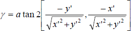
and σ = ± 1.

Substituting any one of these solutions back into Equations (1c) and (1d) gives us:

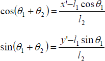
\begin{array}{l} \cos (θ_{1} + θ_{2}) = \frac{x' - l_{1} \cos θ_{1}}{l_{2}} \\ \sin (θ_{1} + θ_{2}) = \frac{y' - l_{1} \sin θ_{1}}{l_{2}} \end{array}

Hence:

θ_{2} = a \tan 2 [\frac{y' - l_{1} \sin θ_{1}}{l_{2}}, \frac{x' - l_{1} \cos θ_{1}}{l_{2}}] - θ_{1}

(1g)

and:

θ_{3} = Ф - θ_{1} - θ_{2}

(1h)

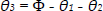
Equations (1f), (1g) and (1h) are the forward kinematics solution for the 3-R manipulator. For a given end effector's position and orientation, there are two different ways of reaching it, each corresponding to a different value of σ. These different configurations are shown in Figure 2:

In this paper, the testing data was taken from training data. In general, because the forward kinematics of a 6-DOF robot arm is a nonlinear mapping from a (X, Y, Z, φ_x, φ_y, and φ_z) space to a (θ₁, θ₂, θ₃, θ₄, θ₅ and θ₆) space, it can be regarded as an input-output process with an unknown transfer function. the approximation of such a relationship is an example of the general approximation problem and as such it is well-suited to learning by an adaptive MIMO NARX neural model. Two problems encountered when teaching a NN robot forward kinematics are the low accuracy of approximation and the need to create a teaching data set with a relatively large number of data points. In the case, where the kinematic parameters of each robot link are known, a simple kinematic model of the 3-DOF robot can be made based on Equations 1(f) to 1(h) and a required number of data points can be readily generated. In the case where the joint parameters are unknown, the required data has to be obtained by measuring the position and orientation of the robot gripper although with a number of arm configurations. Such measurement is very difficult in practice.

3. Proposed Adaptive Forward Neural Mimo Narx (Fnmn) Model of the Nonlinear Forward Kinematics of the Industrial 3-Dof Robot Arm System

The adaptive Forward Neural MIMO NARX (FNMN) model used in this paper is a combination of the Multi-Layer Perceptron Neural Networks (MLPNNs) structure and the Auto-Regressive with eXogenous input (ARX) model. Due to this combination, the proposed Forward Neural MIMO NARX (FNMN) model possesses a powerful universal approximating feature from the MLPNN structure and a strong predictive feature from the nonlinear ARX model.

A fully connected 3-layer feed-forward MLP-network with n inputs, q hidden units (also called “nodes” or “neurons”) and m output units is shown in Fig. 3.

In Figure 1, w₁₀,.., w_q0 and W₁₀,..,W_m0 are the weighting values of the bias neurons of the input layer and the hidden layer respectively.

Figure 1.

Schematic of a robot arm with three revolute joints.

Figure 2.

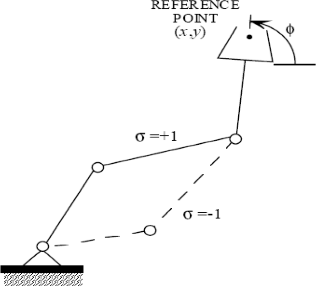
The two Forward kinematics solutions for the 3-R manipulator

Figure 3.

Structure of the feed-forward MLPNN.

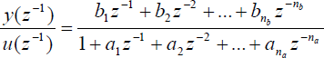
We consider an Auto-Regressive with eXogenous input (ARX) model with noisy input, which can be described as:

A (q^{- 1}) y (t) = B (q^{- 1}) u (t - T) + C (q^{- 1}) e (t)

(2)

with $\begin{array}{l} A (q^{- 1}) = 1 + a_{1} q^{- 1} + a_{2}^{} q^{- 2} \\ B (q^{- 1}) = b_{1} + b_{2} q^{- 1} \\ C (q^{- 1}) = c_{1} + c_{2} q^{- 1} + c_{3} q^{- 2} \end{array}$

where e(t) is the white noise sequence with a zero mean and unit variance, u(t) and y(t) are the input and output of the system respectively, q is the shift operator and T is the time delay.

From Equation (2), and not considering the noise component e(t), we have the general form of the discrete ARX model in a z-domain (with the time delay T=n_k=1):

\frac{y (z^{- 1})}{u (z^{- 1})} = \frac{b_{1} z^{- 1} + b_{2} z^{- 2} + \dots + b_{n_{b}} z^{- n_{b}}}{1 + a_{1} z^{- 1} + a_{2} z^{- 2} + \dots + a_{n_{a}} z^{- n_{a}}}

(3)

in which n_a and n_b are the order of output y(z⁻¹) and input u(z⁻¹) respectively.

This paper investigates the potentiality of various simple adaptive Neural MIMO NARX models in order to exploit them in modelling, identification and control. The forward kinematic model of the industrial 3-DOF robot arm is investigated. Thus, by embedding a 3-layer MLPNN (with the number of neurons of the hidden layer equal 5) in a 1^st-order ARX model, its characteristic equation induced from (3) is as follows:

\begin{array}{l} y h a t (k) = b_{11} q_{1} (k) + b_{12} q_{2} (k) + b_{13} q_{3} (k) - \\ - a_{11} y (k - 1) - a_{12} x (k - 1) \\ x h a t (k) = b_{21} q_{1} (k) + b_{22} q_{2} (k) + b_{23} q_{3} (k) - \\ - a_{21} y (k - 1) - a_{22} x (k - 1) \end{array}

(4a)

We will design the proposed Forward Neural MIMO NARX11 (FNMN11) model (with n_a = 1, n_b = 1, n_k =1) for the industrial 3-DOF robot arm with 5 inputs (including q₁(k), q₂(k), q₃(k), recurrent delayed values y(k-1), x(k-1)), and 2 output values (y_hat(k), x_hat(k)). We recall that three input values q₁(k), q₂(k) and q₃(k) represent the three joint angles [rad] of the 3-DOF robot arm and the two output values y_hat(k) and x_hat(k) represent the Cartesian coordinates (x,y) of the 3-DOF robot arm end-effector respectively. Its structure is shown in Fig. 4a.

Figure 4a.

Structure of the proposed Forward Neural MIMO NARX11 (FNMN11) model.

In this way, the parameters a₁₁, a₁₂, b₁₁, b₁₂, b₁₃ and a₂₁, a₂₂, b₂₁, b₂₂, b₂₃ of the ARX structure of the output variables y_hat(t) and x_hat(t), respectively, become adaptively nonlinear and will be determined from the weighting values W_ij and w_jl of the proposed Neural MIMO NARX11 model. This feature makes the adaptive Neural MIMO NARX model very powerful for modelling, identification and for model-based advanced control as well.

In the same way, we will design the proposed Forward Neural MIMO NARX22 (FNMN22) model (with n_a = 2, n_b = 2, n_k =1) for the industrial 3-DOF robot arm by embedding a 3-layer MLPNN (with the number of neurons of the hidden layer equal 5) in a 2^nd-order ARX model with its characteristic equation induced from (3) as follows:

\begin{array}{l} y h a t (k) = b_{11} q_{1} (k) + b_{12} q_{2} (k) + b_{13} q_{3} (k) + b_{14} q_{1} (k - 1) + b_{15} q_{2} (k - 1) + \\ + b_{16} q_{3} (k - 1) - a_{11} y (k - 1) - a_{12} x (k - 1) - a_{13} y (k - 2) - a_{14} x (k - 2) \\ x h a t (k) = b_{21} q_{1} (k) + b_{22} q_{2} (k) + b_{23} q_{3} (k) + b_{24} q_{1} (k - 1) + b_{25} q_{2} (k - 1) + \\ + b_{26} q_{3} (k - 1) - a_{21} y (k - 1) - a_{22} x (k - 1) - a_{23} y (k - 2) - a_{24} x (k - 2) \end{array}

(4b)

In this way, the proposed Forward Neural MIMO NARX22 (FNMN22) model (n_a = 2, n_b = 2, n_k =1) for the industrial 3-DOF robot arm illustrated in Fig. 4b is composed of 16 inputs (including q₁(k), q₂(k), q₃(k), q₁(k-1), q₂(k-1), q₃(k-1), recurrent delayed values y(k-1), x(k-1), y(k-2), x(k-2)), and 2 output values (y_hat(k), x_hat(k)). We should once more recall that the three input values q₁(k), q₂(k) and q₃(k) represent the three joint angles [rad] of the 3-DOF robot arm and the two output values y_hat(k) and x_hat(k) represent the Cartesian coordinates (x,y) of the industrial 3-DOF robot arm end-effector, respectively. Its structure is shown in Fig. 4b.

Figure 4b.

Structure of the proposed Forward Neural MIMO NARX22 (FNMN22) model.

Furthermore, the class of MLPNN-networks considered in this paper is confined to those having only one hidden layer and using sigmoid activation functions. From Figure 3, the predictive output value ŷ(t) (or y_hat(t)) is calculated as follows:

\begin{array}{l} {\hat{y}}_{i} (w, W) = F_{i} (\sum_{j = 1}^{q} W_{i j} O_{j} (w) + W_{i 0}) = \\ F_{i} (\sum_{j = 1}^{q} W_{i j} . f_{j} (\sum_{l = 1}^{n} w_{j l} z_{l} + w_{j 0}) + W_{i 0}) \end{array}

(5)

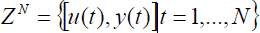
The weights (specified by the matrices w and W ) are the adjustable parameters of the network and they are determined from a set of examples through a process called training. The exemplars – or the training data, as they are usually called – are a set of inputs, u(t) and corresponding desired outputs, y(t).

We specify the training set by:

Z^{N} = {[u (t), y (t)] | t = 1, \dots, N}

(6)

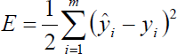
The objective of training is then to determine a mapping from the set of training data to the set of possible weights, $Z^{N} \to \hat{θ}$ , so that the network will produce predictions ŷ(t), which in some sense are “closest” to the true joint angle outputs y(t) of the PAM robot arm.

The prediction error approach, which is the strategy applied here, is based on the introduction of a measure of closeness in terms of a mean sum of a square error (MSSE) criterion:

E_{N} (θ, Z^{N}) = \frac{1}{2 N} \sum_{t = 1}^{N} {[y (t) - \hat{y} (t | θ)]}^{T} [y (t) - \hat{y} (t | θ)]

(7)

Based on the conventional error Back-Propagation (BP) training algorithms, the weighting value is calculated as follows:

W (k + 1) = W (k) - λ \frac{\partial E (W (k))}{\partial W (k)}

(8)

where k is the k^th iterative step of the calculation and λ is the learning rate, which is often chosen as a small constant value.

More concretely, the weights W_ij and w_jl of the neural NARX are then updated as:

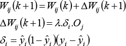
\begin{array}{l} W_{i j} (k + 1) = W_{i j} (k) + Δ W_{i j} (k + 1) \\ Δ W_{i j} (k + 1) = λ . δ_{i} . O_{j} \\ δ_{i} = {\hat{y}}_{i} (1 - {\hat{y}}_{i}) (y_{i} - {\hat{y}}_{i}) \end{array}

(9)

where δ _i is the search direction value of the i^th neuron of the output layer (i=[1 → m]), O_j is the output value of the j^th neuron of the hidden layer (j=[1 → q]), y_i and ŷ_i are the real and predicted outputs, respectively, of the i^th neuron of output layer (i=[1 → m]), and:

\begin{array}{l} w_{j l} (k + 1) = w_{j l} (k) + Δ w_{j l} (k + 1) \\ Δ w_{j l} (k + 1) = λ . δ_{j} . u_{l} \\ δ_{j} = O_{j} (1 - O_{j}) \sum_{i = 1}^{m} δ_{i} W_{i j} \end{array}

(10)

in which δ_j is the search direction value of the j^th neuron of the hidden layer (j=[1 ^→ q]), O_j is the output value of the j^th neuron of the hidden layer (j=[1 ^→ q]), and u_l is the input of the l^th neuron of the input layer (l=[1 ^→ n]). These results by Equations (9) and (10) are demonstrated as follows in the case of the sigmoid being the activation function of the hidden and output layers. Consider the case of the output layer and the error to be minimized:

E = \frac{1}{2} \sum_{i = 1}^{m} {({\hat{y}}_{i} - y_{i})}^{2}

(11)

Using the chain rule method, we have:

\frac{\partial E}{\partial W_{i j}} = \frac{\partial E}{\partial {\hat{y}}_{i}} \frac{\partial {\hat{y}}_{i}}{\partial S_{i}} \frac{\partial S_{i}}{\partial W_{i j}}

(12)

From Equation (11), the following equation is derived:

\frac{\partial E}{\partial {\hat{y}}_{i}} = ({\hat{y}}_{i} - y_{i})

(13)

with $S_{i} = \sum_{j = 1}^{q} W_{i j} . O_{j} + b i a s_{i}$ as a sum calculation at the i^th node of the output layer and ${\hat{y}}_{i} = \frac{1}{1 + e^{- S_{i}}}$ . This gives:

\frac{\partial {\hat{y}}_{i}}{\partial S_{i}} = \frac{e^{- S_{i}} + 1 - 1}{{(1 + e^{- S_{i}})}^{2}} = \frac{1}{(1 + e^{- S_{i}})} (1 + \frac{- 1}{1 + e^{- S_{i}}}) = {\hat{y}}_{i} (1 - {\hat{y}}_{i})

(14)

\frac{\partial S_{i}}{\partial W_{i j}} = O_{j}

(15)

Replace (13), (14), (15) with (12) and then substitute all of them into (8), then the following equation is derived:

\begin{array}{l} W_{i j} (k + 1) = W_{i j} (k) + Δ W_{i j} (k + 1) \\ Δ W_{i j} (k + 1) = λ . δ_{i} . O_{j} \\ δ_{i} = {\hat{y}}_{i} (1 - {\hat{y}}_{i}) (y_{i} - {\hat{y}}_{i}) \end{array}

(16)

Equation (9) is, therefore, demonstrated.

Using the chain rule method, the same approach is used for updating the weights of the hidden layer, namely:

\frac{\partial E}{\partial w_{j l}} = \frac{\partial E}{\partial O_{j}} \frac{\partial O_{j}}{\partial S_{j}} \frac{\partial S_{j}}{\partial w_{j l}}

(17)

Then:

\begin{array}{l} \frac{\partial E}{\partial O_{j}} = \sum_{i = 1}^{m} [\frac{\partial E}{\partial S_{i}} \frac{\partial S_{i}}{\partial O_{j}}] = \sum_{i = 1}^{m} [\frac{\partial E}{\partial S_{i}} \frac{\partial}{\partial O_{j}} {\sum_{j = 1}^{q} W_{i j} O_{j} + b i a s_{i}}] = \\ \sum_{i = 1}^{m} [\frac{\partial E}{\partial S_{i}} W_{i j}] = \sum_{i = 1}^{m} [- δ_{i} W_{i j}] \end{array}

(18)

with $S_{j} = \sum_{l = 1}^{n} w_{j l} . u_{l} + b i a s_{j}$ as the sum calculation at the j^th node of the hidden layer and $O_{j} = \frac{1}{1 + e^{- S_{j}}}$ . We obtain:

\frac{\partial O_{j}}{\partial S_{j}} = \frac{e^{- S_{j}} + 1 - 1}{{(1 + e^{- S_{j}})}^{2}} = \frac{1}{(1 + e^{- S_{j}})} (1 + \frac{- 1}{1 + e^{- S_{j}}}) = O_{j} (1 - O_{j})

(19)

\frac{\partial S_{j}}{\partial w_{j l}} = u_{l}

(20)

Replace (18), (19), (20) with (17) and then substitute all of them into (8). The following equation is derived:

\begin{array}{l} w_{j l} (k + 1) = w_{j l} (k) + Δ w_{j l} (k + 1) \\ Δ w_{j l} (k + 1) = λ . δ_{j} . u_{l} \\ δ_{j} = O_{j} (1 - O_{j}) \sum_{i = 1}^{m} δ_{i} W_{i j} \end{array}

(21)

Equation (10) is thus demonstrated.

4. Modelling and Identification Results

In general, the procedure which must be executed when attempting to identify a dynamical system consists of four basic steps: •

STEP 1 (Getting the Training Data)

•

STEP 2 (Selecting the Model Structure)

•

STEP 3 (Estimating the Model)

•

STEP 4 (Validating the Model)

In Step 1, the identification procedure is based on experimental input-output data values measured from the forward kinematics of the industrial 3-DOF robot arm system. The input signals θ₁, θ₂ and θ₃ (or q₁(k), q₂(k) and q₃(k) in the z-domain) represented the joint-angles applied to the three joints of the industrial robot arm in order to obtain a circular trajectory from the output signals (x,y) represented by the Cartesian coordinates of the end-effecter of the industrial 3-DOF robot arm. Thus, the responding output Cartesian coordinates (x,y) are chosen to formulate a circular trajectory of the robot arm's end-effecter. Figure 5a presents the collected input-output data composed of the three θ₁, θ₂ and θ₃ angle inputs applied to the three joints of the industrial 3-DOF robot arm system and the responding x(t) and y(t) outputs of the industrial robot arm's end-effector Cartesian coordinates.

Figure 5a.

Training data composed of (θ₁, θ₂ and θ₃) inputs and (x, y) outputs the for identification process.

This collected input-output data is used for training and validating the proposed Forward Neural MIMO NARX (FNMN) model. The Cartesian coordinates (x,y) considered as reference outputs and the forward kinematics of the industrial 3-DOF robot arm angles (θ₁, θ₂ and θ₃) are considered as reference inputs. Figure 5a shows that the input signals θ₁, θ₂ and θ₃ (or q₁(k), q₂(k) and q₃(k) in the z-domain) represent joint-angles applied to the three joints of the industrial robot arm and the output signals (x,y) represent the Cartesian coordinates of the end-effecter of the industrial 3-DOF robot arm. From Figure 5a, we have the (θ₁, θ₂, and θ₃) reference inputs (corresponding to q₁(k), q₂(k) and q₃(k) in the z-domain) and (x,y) considered as reference outputs from (0–1) [s] are used for training, while the (x,y) reference outputs and the 3-DOF robot arm joint-angle inputs (θ₁, θ₂ and θ₃) from (1–2)[s] used for validation purpose.

Back Propagation (BP) learning algorithm based on the error between the reference coordinates (x,y) collected from the industrial 3-DOF robot arm system and the responding Cartesian coordinates (x_h, y_h) collected from the designed FNMN model to update the weights of the proposed adaptive forward neural MIMO NARX model. Figure 5b and Figure 5c illustrate the identification scheme of the industrial 3-DOF robot arm using the proposed Forward Neural MIMO NARX11 (FNMN11) and Forward Neural MIMO NARX22 (FNMN22) models respectively.

Figure 5b.

Identification scheme of the industrial 3-DOF robot arm using the proposed FNMN11 model.

Figure 5c.

Identification scheme of the industrial 3-DOF robot arm using the Forward Neural MIMO NARX22 model.

The second step relates to the selection of the model structure. The proposed Forward Neural MIMO NARX11 (FNMN11) and Forward Neural MIMO NARX22 (FNMN22) model structures are attempted. The block diagrams in Figure 5b and Figure 5c illustrate the identification scheme of these two proposed FNMN models. Figure 4a and Figure 4b illustrate the final Forward Neural MIMO NARX11 and Forward Neural MIMO NARX22 model structures of these two proposed FNMN models.

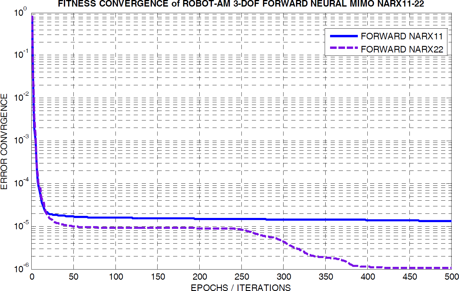
The third step estimates the values for the trained Forward Neural NARX model. The optimal fitness value for the BP-based optimization and identification process is calculated. The estimation result is presented in Figure 6. This figure represents the fitness convergence values of the proposed forward kinematics of the industrial 3-DOF robot arm system which correspond to two different FNMN models (Forward Neural NARX11 and Forward Neural NARX22 models) and all two were identified and optimized with the Back Propagation (BP) learning algorithm. A good convergence of the minimized fitness value after 500 training iterations is shown in Figure 6 with a perfect Mean Sum of Scaled Error (MSSE) = 0.000016 and MSSE = 0.0000012 with the proposed FNMN11 and FNMN22 model respectively. The training result shows that proposed Forward Neural MIMO NARX (FNMN) model, with an MSSE value which is perfectly minimized, ensures to learn well dynamic and nonlinear features of the industrial 3-DOF robot arm.

These good results are attributed to how the proposed FNMN model combines the extraordinary approximating capability of the neural system with the powerful predictive and adaptive potentiality of the nonlinear NARX structure that is implied in the FNMN model. Consequently, the BP-based Forward kinematics of the industrial robot arm FNMN model addresses all of the nonlinear features of the forward kinematics of the industrial robot arm system that are implied in the input angle signals (θ₁, θ₂ and θ₃) and the responding output Cartesian co-ordinates (x,y).

The last step relates to the validating of the resulting nonlinear FNMN models. Applying the same training diagram in Figure 5b and Figure 5c, a good validating result demonstrates the performance of the resulting Forward Neural MIMO NARX model, as presented in Figure 7 and Figure 8. The error optimized nearly zero between the real industrial 3-DOF robot arm system responding (x,y) and the Forward Neural MIMO NARX model responding (x_h, y_h) asserts the very good performance of proposed FNMN model. The error shown in Figure 7 and Figure 8 emphasises the fact that the quality of the Forward Neural MIMO NARX22 model is similar to the Forward Neural MIMO NARX11 model.

Figure 6.

Fitness convergence of the forward kinematics of the industrial robot arm: a) the Forward Neural MIMO NARX11 model; b) the Forward Neural MIMO NARX22 model.

Figure 7.

Validation of the proposed forward kinematics of the industrial 3-DOF robot arm: a) Forward Neural MIMO NARX11 model; b) Forward Neural MIMO NARX22 model.

Figure 8.

Validation of the proposed forward kinematics of the industrial 3-DOF robot arm: a) Forward Neural MIMO NARX11 model; b) Forward Neural MIMO NARX22 model.

Finally, Figure 9 and Figure 10 illustrate the auto-tuning variation of the adaptive ARX parameters of the proposed Forward Neural MIMO NARX11 and NARX22 models of the industrial 3-DOF robot arm. In essence, the ten parameters a₁₁, a₁₂, b₁₁, b₁₂, b₁₃, and a₂₁, a₂₂, b₂₁, b₂₂, b₂₃ of the two 1^st-order ARX structure integrated in the proposed FNMN11 model were adaptively auto-tuned, as illustrated in Figure 9. Similarly, the twenty parameters a₁₁, a₁₂, a₁₃, a₁₄, b₁₁, b₁₂, b₁₃, b₁₄, b₁₅, b₁₆ and a₂₁, a₂₂, a₂₃, a₂₄, b₂₁, b₂₂, b₂₃, b₂₄, b₂₅, b₂₆ of the two 2^nd-order ARX structures integrated in the proposed FNMN22 model were adaptively and flexibly auto-tuned, as illustrated in Figure 10. These results show that the parameters of the ARX structure integrated in the proposed FNMN models now become adaptively nonlinear and will be adaptively determined from the optimized weighting values W_ij and w_jl of the Neural MIMO NARX model. This feature once more proves that the proposed adaptive Forward Neural MIMO NARX (FNMN) model is very powerful and adaptive for identification and model-based advanced control.

Figure 9.

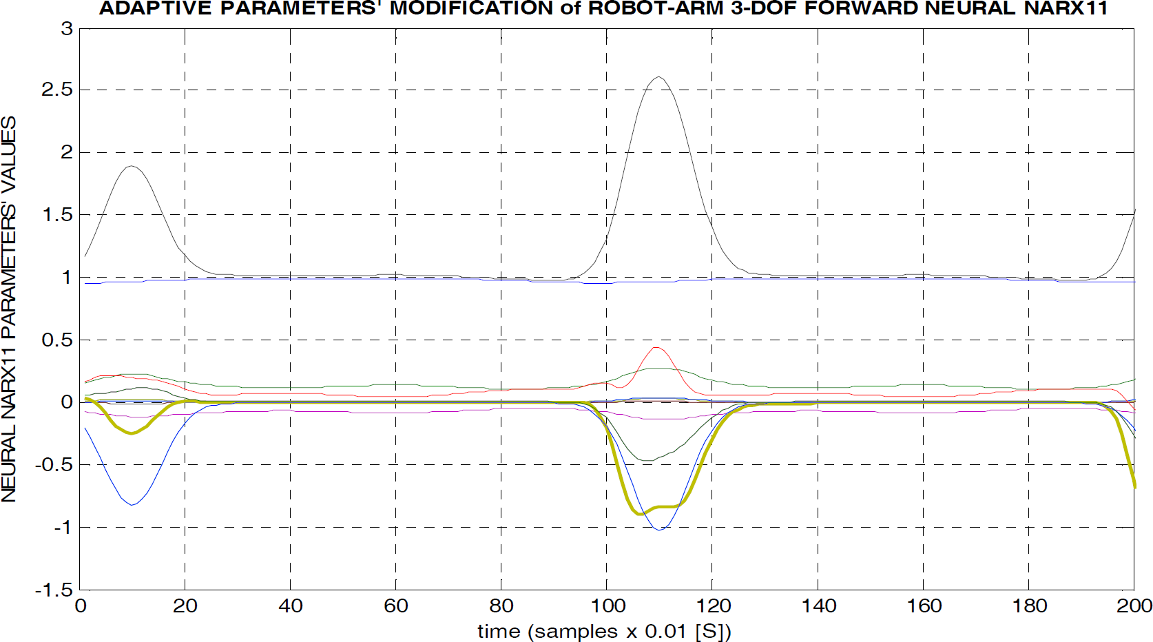
Adaptive Parameters of the ARX Structure embedded in the proposed FNMN11 model.

Figure 10.

Adaptive Parameters of the ARX Structure embedded in the proposed FNMN22 model.

In summary, Table 1 and Table 2 tabulate the optimized weighting values of the proposed Forward Neural MIMO NARX11 and Forward Neural MIMO NARX11 models. The final structures of the Forward Neural MIMO NARX11 and Forward Neural MIMO NARX22 models which were identified and optimized by the BP learning algorithm are shown in Figure 4a and Figure 4b respectively.

Table 1.

Optimized weights of the Forward NEURAL MIMO-NARX11 – Total Number of weighting values = 57.

Table 2.

Optimized weights of the Forward NEURAL MIMO-NARX22 – Total Number of weighting values = 97.

5. Conclusions

In this paper, a new approach in the form of a Forward Neural MIMO NARX (FNMN) model is introduced for the modelling and identification of the forward kinematics of the industrial robot arm-based intelligent actuator. The training and testing results show that the newly proposed forward dynamic neural MIMO NARX model presented in this paper can be used in online control with better dynamic properties and with significant robustness. This resulting proposed intelligent model is quite suitable for application in the modelling, identification and control of various complex plants, including linear and nonlinear processes, and without concern for any large change in the external environment.

Footnotes

6. Acknowledgments

This research was completely supported by the NAFOSTED (Vietnam).

References

Alavandar

and Nigam

M. J.

“Neuro-Fuzzy based Approach for Forward Kinematics Solution of Industrial Robot Manipulators”, Int. J. of Computers, Communications & Control, ISSN 1841-9836, Vol. III, 2008, No. 3, pp. 224–234.

Morris

A. S.

and Mansor

. “Artificial neural network for finding Forward kinematics of robot manipulator using look up table”, Journal of Robotica, 1997, Vol. 15, pp 617–625.

Ahmad

and Guez

. “On the Solution to the Inverse Kinematic Problem”, in Proceedings of Robotics and Automation International Conference, 1990, vol.3, pp.1692–1697.

Karlik

Bekir

& Aydin

Serkan

, “An improved approach to the solution of kinematics problems for robot manipulator,” Journal Engineering Applications of Artificial Intelligence, vol.13, 2000, pp. 159–164.

Al-Gallaf

E. A.

, “Neural Networks for Multi-Finger Robot Hand Control”, JKAU: Eng. Sci., Vol. 19 No. 1, 2008, pp. 19–42.

Manocha

and Canny

J.F.

“Efficient Inverse kinematics for a general 6R manipulator”, IEEE Transaction on Robotics and Automation, 1994, vol.10, Issue 5, pp. 648–657.

Kozakiewicz

Ogiso

and Miyake

“Partitioned Neural Network architecture for Inverse Kinematic calculation of a 6 dof robot manipulator”, in Proceedings of IEEE International Joint Conference on Neural Networks, 1991, vol.3, pp.2001–2006.

Mayorga

and Sanongboon

“Forward kinematics and geometrically bounded singularities prevention of redundant manipulators: An Artificial Neural Network approach”. In Journal of Robotics and Autonomous Systems, vol. 53, 2005, pp. 164–176.

Kieffer

Morellas

and Donath

“Neural Network Learning of the Inverse Kinematic Relationships for a Robot Arm”

Proceedings of the 1991 IEEE Intemational conference on Robotics and Automation, Sacramento, Califomia – April 1991, vol. 3, pp. 2418–2425.

10.

Rao

D. H.

and Gupta

M.M.

“Performance Comparison of Dynamic Neural Networks as Applied to Robot Inverse Kinematic Computations”. Proceedings of the American Control Conference Baltlmorr, Mayland, June 1994, vol. 2, pp. 2153–2157.

11.

Velagic

Osmic

and Lacevic

“Neural Network Controller for Mobile Robot Motion Control”. International Journal of Intelligent Systems and Technologies (WASET), vol. 47, 2008, pp. 193–198.

12.

Sadjadian

Taghirad

H.D.

and Fatehi

“Neural Networks Approaches for Computing the Forward Kinematics of a Redundant Parallel Manipulator”. International Journal of Computational Intelligence, 2005, pp. 53–61.

13.

Ding

, and Wang

“Recurrent Neural Networks for Minimum Infinity-Norm Kinematic Control of Redundant Manipulators”. IEEE Transaction on Systems, Man, and Cybernetics, Part-A: Systems and Humans, vol.29, No.3, May 1999, pp. 269–276.

14.

Ahn

K.K.

Anh

H.P.H.

, “A new approach of modeling and identification of the pneumatic artificial muscle (PAM) robot arm based on recurrent neural network,” In Proceedings IMechE, Part I: Journal of Systems and Control Engineering, 2007, 221(I8), pp.1101–1122.

15.

Ahn

K.K.

, and Anh

H.P.H.

, “Identification of the pneumatic artificial muscle manipulators by MGA-based nonlinear NARX fuzzy model,” IFAC Journal of MECHATRONICS, February 2009, Vol. 19, Issue 1, pp. 106–133.

16.

Ahn

K.K.

, and Anh

H.P.H.

, “Forward Double NARX Fuzzy Model for System Identification,” IEEE/ASME Journal of MECHATRONICS, February 2010, Vol. 15, Issue 1, pp. 136–148.

Novel Adaptive Forward Neural MIMO NARX Model for the Identification of Industrial 3-DOF Robot Arm Kinematics

Abstract

Keywords

1. Introduction

2. Forward Kinematics of the Industrial 3-Dof Robot Arm System

3. Proposed Adaptive Forward Neural Mimo Narx (Fnmn) Model of the Nonlinear Forward Kinematics of the Industrial 3-Dof Robot Arm System

4. Modelling and Identification Results

5. Conclusions

Footnotes

6. Acknowledgments

References