Sage Journals: Discover world-class research

Abstract

Real systems are usually non-linear, ill-defined, have variable parameters and are subject to external disturbances. Modelling these systems is often an approximation of the physical phenomena involved. However, it is from this approximate system of representation that we propose - in this paper - to build a robust control, in the sense that it must ensure low sensitivity towards parameters, uncertainties, variations and external disturbances. The computed torque method is a well-established robot control technique which takes account of the dynamic coupling between the robot links. However, its main disadvantage lies on the assumption of an exactly known dynamic model which is not realizable in practice. To overcome this issue, we propose the estimation of the dynamics model of the nonlinear system with a machine learning regression method. The output of this regressor is used in conjunction with a PD controller to achieve the tracking trajectory task of a robot manipulator. In cases where some of the parameters of the plant undergo a change in their values, poor performance may result. To cope with this drawback, a fuzzy precompensator is inserted to reinforce the SVM computed torque-based controller and avoid any deterioration. The theory is developed and the simulation results are carried out on a two-degree of freedom robot manipulator to demonstrate the validity of the proposed approach.

Keywords

Two-degree of Freedom Robot Manipulator Inverse Dynamics Control Support Vector Machine (SVM)Fuzzy Precompensator

1. Introduction

For many years, the problem of controlling highly non-linear systems has received much attention within the control community, especially fast manipulation control. As a result of the strong need to find easy and robust methods to control robots, many solutions have been proposed. When the controlled part of the process is slightly disturbed, classical control laws - such as PID - may be sufficient if the accuracy requirements and system performance are not too severe. Otherwise, control laws must be developed that ensure the robustness of the processes' behaviour in the face of parameter uncertainties and variations.

One of the most popular and famous techniques is inverse dynamics control - also called the computed torque control. Borrowed from the rigid robot manipulator [1], it can be easily applied to many other nonlinear systems [2]. This technique offers a wide variety of advantages. However, it requires precise knowledge of the analytical model of the system in order to compute the feed-forward torques required for the execution of trajectory tracking. Nevertheless, the dynamics of robot manipulators are coupled and highly nonlinear. They contain uncertainties such as friction and un-modelled nonlinearities. This is why a precise model cannot be obtained and why many efforts have been deployed to solve the problem of dynamic uncertainties. Many robot adaptive controllers have been proposed to solve the problem of parameter uncertainties and disturbances. However, few have been proposed to deal with both dynamic and kinematics uncertainties [3, 4]. To deal with these issues, researchers have demonstrated the positive use of neural networks in learning system uncertainties [5] and in helping in the generation of control laws [6, 7, 8]. In fact, instead of generating the feed-forward signal mathematically, it can be learnt from the feedback signal using neural networks. However, neural networks often suffer from the curse of dimensionality and the over-fitting problem. The theory and application of fuzzy logic is another tool used to control such highly nonlinear systems [9, 10]. It uses fuzzy linguistic variables and fuzzy logic to allow for smooth interpolation. Fuzzy logic is an alternative way to model human expertise. In [11], the authors combined the advantages of fuzzy and neural network intelligence to improve the overall learning ability and achieve robust control. In our previous work [12], we combined a PID controller with a fuzzy precompensator to control a robot manipulator tracking a pre-specified trajectory. We used fuzzy logic to design a precompensator on the basis of decision-making rules. It is tuned to minimize the output error when the PID controller exhibits significant steady-state error. However, fuzzy control methodology requires the tuning of membership functions and may not scale well to complex systems. It deals with imprecision and vagueness, but not with uncertainty.

Recently, Support Vector Machines (SVMs) have been introduced by Vapnik as an intriguing alternative machine learning method. They were originally designed for pattern recognition and classification tasks [13], and have been successfully used in a wide variety of classification problems, such as 3D object recognition [14], biomedical imaging [15], image compression [16] and remote sensing [17]. Furthermore, they exhibit very interesting behaviours when extended to solve regression and function approximation problems. SVMs do not suffer from the over-fitting problem and have a good generalization property. SVMs are based on the idea of structural risk minimization, which shows that the generalization error is bounded by the sum of the training error and a term depending on the Vapnik–Chervonenkis dimension. By minimizing this bound, high generalization capabilities can be achieved. In [18], the authors survey recent developments in the research and application of SVMs in intelligent robot information acquisition and processing. A comparison between two non-parametric regression methods for model approximation is proposed [19]. The outcomes yield positive results to the detriment of high computational cost.

Based on the work of Cheah et al. [20], in which they propose an adaptive Jacobian controller for the trajectory tracking of robot with uncertain kinematics and dynamics, we propose to exploit support vector regression for designing an efficient and robust control law to track robot trajectories. As an extension to our previous results [21], this paper studies this subject thoroughly. Uncertainties in robot parameters and nonlinearities can be dealt with more efficiently than model-based techniques. To avoid using online learning, we propose offline learning for the model's system. This model is not overly sensitive to disturbances. This is explained by the fact that the complexity of the model's representation by support vectors is independent of the dimensionality of the input space and depends only upon the number of support vectors. To further improve the performance of the above approach and ultimately lessen error bounds in case the robot undergoes changes in its kinematic and/or dynamic parameters, a fuzzy precompensator is inserted as reinforcement to the proposed scheme [12]. Simulations are carried out on a two-degree robot manipulator. The effectiveness of the proposed controller is demonstrated for different operating conditions and the results are very satisfactory. This paper is organized as follows: Section 2 formulates the robot dynamic equations; Section 3 presents the inverse dynamic control concept; Section 4 presents the SVM regression technique and model estimation with non-parametric regression techniques; Section 5 presents the development of the fuzzy precompensator; Section 6 describes the way the fuzzy rule base is obtained using evolutionary programming; Section 7 reports the simulations' results and how the proposed approach provides positive outcomes, thereby justifying their applicability; finally, Section 8 concludes the paper.

2. Problem formulation

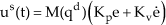
The dynamic equations of the robot manipulator are found through the use of the Lagrangian formulation, and the dynamic equation of an n-degree of freedom manipulator can be written as:

τ = M (q) \overset{..}{q} + C (q, \dot{q}) \dot{q} + G (q) + F (\dot{q})

(1)

where q ∈ ℜⁿ is the generalized joint coordinate; M(q) ∈ ℜ^n×n is the symmetric positive definite inertia matrix, bounded as mI ≤ M(q) ≤ m̄ (q)I for some constant m and function m̄(q), vector C(q,q̇)q̇ ∈ ℜⁿ presents the centrifugal and Coriolis torques, bounded as ‖C(q,q̇)| ≤ a₁‖q̇|, the terms G(q) ∈ ℜⁿ and F(q) ∈ ℜⁿ are the vectors of gravitational torques and friction respectively, bounded as ‖G(q) + F(q̇)‖ ≤ a₂ + a₃‖q̇|, and τ ∈ ℜⁿ is the vector of applied joint torques. The design of the controllers for the fine motion of the manipulator may be considered in two stages: the primary controller, which is nothing but the inverse dynamics of the manipulator inserted in the feedforward path to compensate for the nonlinear effects and which attempts to cancel the nonlinear terms in the model. However, the mathematical model used is usually not exact, and since the system is subject to disturbances, undesirable errors can be corrected by means of an additional controller, called a secondary controller (cf. Fig. 1).

Figure 1.

Primary and secondary robot manipulator control

3. Inverse Dynamics Control

Let us consider the robot dynamics given by equation (1). The objective in using the inverse dynamic control is to eliminate the nonlinearities in the dynamics, as shown in Fig. 1. The inverse dynamic control technique is based on a controller command apprehending a priori knowledge about the system written in a dynamic model. This approach is often referred to as the computed torque method. Since the control objective is trajectory tracking in a joint space, the desired trajectories are joint angles, velocities and accelerations. The tracking errors are defined as:

{\begin{cases} e = q^{d} - q \\ \dot{e} = {\dot{q}}^{d} - \dot{q} \end{cases}

(2)

where the measurements of q and q̈ are required in the subsequent design. To conform to the inverse nonlinear control given in Fig. 1, we rewrite equation (1) as:

τ = M (q) \overset{..}{q} + V (q, \overset{..}{q})

(3)

where:

V (q, \dot{q}) = C (q, \dot{q}) \dot{q} + G (q) + F (\dot{q})

(4)

V(q,q̇) is a term that contains all the forces acting on the system. The functions C, G and F are defined as above. The problem is to determine the input vector τ(t) so that q(t) will track the desired trajectory q^d(t) with tolerable errors. The input will be generated as :

τ (t) = u^{d} (t) + u^{s} (t)

(5)

where:

u^{d} (t) = M (q^{d}) {\overset{..}{q}}^{d} + V (q^{d}, {\dot{q}}^{d})

(6)

and:

u^{s} (t) = M (q^{d}) (K_{p} e + K_{v} \dot{e})

(7)

q^d, q̇^d and q̈^d denote the desired position, velocity and acceleration, respectively. Under ideal conditions and perfect knowledge of the parameter values with no disturbances, controller (6) causes the exact cancellation of the nonlinear expression in equation (3); that is, if V(q^d,q̇^d) = V(q,q̇), M(q^d) = M(q) and q(0) = q^d(0), then q(t) = q^d(t) for all t ≥ 0. The implementation and the proper operation of the primary controller in equation (6) require that the dynamical model and the numerical values of the parameters are accurately known. If this is not the case, the cancellation of the nonlinear terms may not be perfect. Therefore, the secondary controller given by equation (7) is needed to compensate for the effects of internal modelling errors and disturbances. It will regulate small deviations of the system response about a nominal trajectory. Hence, it will be designed on the basis of a model obtained by the linearizing equation (3) about the pre-specified trajectory. For the analysis of the control system specified by equations (3) and (5), the following equalities are assumed:

V (q^{d}, {\dot{q}}^{d}) = V (q, \dot{q}) ​ ​ a n d ​ ​ M (q^{d}) = M (q))

(8)

After substituting equation (3) into equation (5) and recognizing the relations (8) in the resulting equation, we obtain the following error equation:

\overset{..}{e} + K_{v} \dot{e} + K_{p} e = 0

(9)

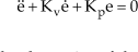
The stability and the dynamics of the error are controlled by the feedback gains K_p and K_v. They can be chosen so that the error equation is stable [1]. They can, for example, be tuned so that the eigenvalues of system in equation (8) assume the values that result in the acceptable responses of the system states. Unfortunately, in practice, robot dynamics cannot be modelled exactly; they are usually subject to torque disturbance and/or modelling errors. In this case, the closed-loop system will be different to that of equation (9). By equating equations (3) and (5) and by taking the estimates of M(q^d) and V(q^d,q̈^d) as M̂(q) and V̂(q,q̈) respectively, we obtain:

\overset{..}{e} + K_{v} \dot{e} + K_{p} e = {\overset{⌢}{M}}^{- 1} (q) [\tilde{M} (q) \overset{..}{q} + \tilde{V} (q, \dot{q}) + ν']

(10)

where M˜(q) = M(q) − M̂(q) and V˜(q,q̇) = V(q,q̇) − V̂(q,q̇) represent errors in the dynamic model. ν′ is a vector function due to all the disturbances being completely unknown, but it is known to be upper bounded. The error equation (10) may be written in the form:

\overset{..}{e} + K_{v} \dot{e} + K_{p} e = {\overset{⌢}{M}}^{- 1} (q) [Y (q, \dot{q}, \overset{..}{q}) \tilde{θ} + ν']

(11)

where $\tilde{θ}$ is the vector of the parameter errors and Y(q,q̇,q̈) is a matrix of functions.

In this work, and instead of using the analytical dynamics model and mathematically computing the required feedforward compensation, we propose to use a kernel regressor to learn the feed-forward torques and a servo feedback control scheme to improve robustness. This may have the advantages of not only approximating and compensating for unknown system functions but also for unknown system properties, such as friction. In this case, and in absence of unknown disturbances, the second term of equation (10) is zero and the stability and the dynamics of the system are governed by equation (9). In the sequel, the learning feed-forward control is developed using the support vector machine (SVM).

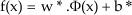
If we approximate the model using a regression technique, equation (5) is changed to:

u = T (q^{d}, {\dot{q}}^{d}, {\overset{..}{q}}^{d}) + \overset{⌣}{M} (q^{d}) (K_{v} \dot{e} + K_{p} e)

(12)

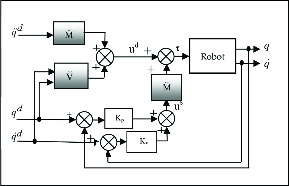
such that T(q^d, q̇^d, q̈^d) = M̆(q^d)q̈^d + V̆(q^d, q̇^d), M̆(q^d) and V̆(q^d, q̇^d) are the approximate of M(q^d) and V(q^d, q̇^d) respectively, determined by an appropriate kernel regressor. Actually, the inverse dynamics control based on SVM models will have the structure shown in Fig. 2.

Figure 2.

SVM-based inverse dynamics control

4. Support Vector Regression and Model Estimation

4.1 Regression with the SVM

For a better understanding of the support vector machine, let us first consider a supervised binary classification problem. Let us assume that the training set consists of N vectors x_i ∈ ℜ^d (i = 1, 2, …, N) from the d-dimensional feature space X. To each vector x_i, we associate a target y_i ∈ {–1, +1}. The linear SVM classification approach consists of looking for a separation between the two classes in X by means of an optimal hyperplane that maximizes the separating margin. In the nonlinear case, which is the most commonly used since the data is often linearly non-separable, they are first mapped with a kernel method in a higher dimensional feature space, i.e. Φ(x) ∈ ℜ^d′ (d′ > d). The membership decision rule is based on the function sgn[f(x)], where f(x) represents the discriminant function associated with the hyperplane in the transformed space and is defined as:

f (x) = w * . Φ (x) + b *

(13)

The optimal hyperplane defined by the weight vector w* ∈ ℜ^d′ and the bias b* ∈ ℜ is that which minimizes a cost function that expresses a combination of two criteria, namely: 1) margin maximization and 2) error minimization. It is expressed as:

Ψ (w, ξ) = \frac{1}{2} {‖ w ‖}^{2} + C \sum_{i = 1}^{N} ξ_{i}

(14)

This cost function minimization is subject to the constraints:

y_{i} (w . ​ Φ (x_{i}) + b) \geq 1 - ξ_{i}, i = 1, 2, \dots, N

(15)

and:

ξ_{i} \geq 0 ​ ​ ​ i = 1, 2, \dots, N

(16)

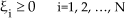
where ξ_i is the so-called slack variable introduced to account for non-separable data. The constant C represents a regularization parameter that allows the control of the shape of the discriminant function and, consequently, the decision boundary when data is non-separable. The above optimization problem can be reformulated through a Lagrange function for which the Lagrange multipliers can be found by means of a dual optimization leading to a quadratic programming solution [22], i.e.:

\underset{α}{m a x} \sum_{i = 1}^{N} α_{i} - \frac{1}{2} \sum_{i, j = 1}^{N} α_{i} α_{j} y_{i} y_{j} K (x_{i}, x_{j})

(17)

Under the constraints:

α_{i} \geq 0, i = 1, 2, \dots, N

and:

\sum_{i = 1}^{N} α_{i} y_{i} = 0

where α = [α₁, α₂, …, α_N] is the vector of the Lagrange multipliers. The final result is a discriminant function conveniently expressed as a function of the data in the original dimensional feature space X.

Now, rather than dealing with outputs y ∈ {±1}, regression estimation is concerned with estimating real valued functions. The SVM regression technique stems from the idea of deducing an estimate ĝ(x) of the true and unknown relationship y = g(x) between the vector of observations x and the desired biophysical parameter y from a given set of N_T training samples. In our case, N_T will include labelled as well as semi-labelled samples, such that ĝ(x), first, has a maximum deviation from the desired targets y_i, (i=1,…, N_T) and, second, is as smooth as possible [22]. This is usually performed by mapping the data from the original d-dimensional feature space to a higher dimensional transformed feature space - i.e., Φ(x) ∈ ℜ^d′ (d′ > d) - in order to increase the flatness of the function and to approximate it in a linear way as follows:

\hat{g} (x) = w * . Φ (x) + b *

(18)

where w* is a vector of weights and b* is the offset. ‘Flatness’ means that one seeks a small w, and one way to ensure this is by minimizing the norm - i.e. ‖ w ‖². The optimal linear function in the higher dimensional transformed feature space is that which minimizes the following cost function:

Ψ (w, ξ) = \frac{1}{2} {‖ w ‖}^{2} + C \sum_{i = 1}^{N_{T}} (ξ_{i} + ξ_{i}^{*})

(19)

Subject to the following constraints:

{\begin{matrix} y_{i} - (w . Φ (x_{i}) + b) \leq ε + ξ_{i} \\ (w . Φ (x_{i}) + b) - y_{i} \leq ε + ξ_{i}^{*} \\ ξ_{i}, ξ_{i}^{*} \geq 0 \end{matrix}; i = 1, 2, \dots, N_{T}

(20)

where ε > 0 is a predefined constant which controls the noise tolerance. The ξ_i and ξ*_i are the so-called slack variables introduced to account for those samples that do not lie in the ε-deviation tube, the constant C represents a regularization parameter that allows the tuning of the tradeoff between the flatness of the function ĝ(x) and the amount up to which deviations larger than ε are tolerated. It is well known that ε is proportional to the input noise level and should also depend on the number of training samples [23, 24]. The above optimization problem reformulated through a Lagrange function into a dual optimization problem leads to a solution that is a function of the data conveniently expressed in the original dimensional feature space as:

\hat{g} (x) = \sum_{i \in W} (α_{i} - α_{i}^{*}) K (x_{i}, x) + b^{*}

(21)

where K(·,·) is a kernel function and W is the subset of indices (i=1, 2, …, N_T) corresponding to the non-zero Lagrange multipliers α_i or α_i*'s. The training samples associated to non-zero weights are called support vectors. The kernel K(·,·) should be chosen so that it satisfies the condition imposed by Mercer's theorem [25, 26]. Examples of common nonlinear kernels that fulfil Mercer's condition are the polynomial and the Gaussian kernel functions.

4.2 Robot Model Estimation with Support Vector Regression

In this second part of the section, we will generate the approximate model of the robot manipulator with nonparametric regression techniques. We consider a two-link robot manipulator whose dynamics equations are derived using the Euler-Lagrange formulation. Based on relation (6), the equations of the motion of the two-link manipulator are expressed for each joint as:

\begin{array}{l} u_{1}^{d} = τ_{1} + τ_{2} \\ u_{2}^{d} = τ_{3} + τ_{4} \end{array}

(22)

such that

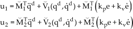
τ₁ = M₁^T(q)q̈^d, τ₂ = V₁(q^d,q̇^d), τ₃ = M^T₂(q)q̈^d, τ₄ = V₂(q^d,q̈^d) where M^T₁ and M^T₂ are the row vectors of the inertia matrix and V₁ and V₂ are vectors regrouping the terms of the Coriolis and centrifugal torques as well as the gravity and friction torques. A model identification procedure is carried out to identify these terms using SVM regression. Each term is identified separately to get - at the end - four approximate models, namely M̆₁, M̆₂, V̆₁ and V̆₂ which are used to generate the following approximate robot manipulator torques:

\begin{array}{l} u_{1} = {\overset{⌣}{M}}_{1}^{T} {\overset{..}{q}}^{d} + {\overset{⌣}{V}}_{1} (q^{d}, {\dot{q}}^{d}) + {\overset{⌣}{M}}_{1}^{T} (k_{p} e + ​ k_{v} \dot{e}) \\ u_{2} = {\overset{⌣}{M}}_{2}^{T} {\overset{..}{q}}^{d} + {\overset{⌣}{V}}_{2} (q^{d}, {\dot{q}}^{d}) + {\overset{⌣}{M}}_{2}^{T} (k_{p} e + k_{v} \dot{e}) \end{array}

(23)

The purpose of the PD-controller is to servo the system so that the actual displacement of the joint will track a desired angular displacement specified by a pre-planned trajectory. The starting point is the use of the desired joint angle, velocity and acceleration trajectories to generate the corresponding torques for every sampling time. The obtained torque vectors are stored with the position, velocity and acceleration vectors in lookup tables to be referred to afterwards by the SVM regressor for training.

The entries of the svmtrain function are, consequently, the torques τ₁ and τ₃, as well as the position and acceleration vectors needed to implement M̆₁ and M̆₂. The torques τ₂ and τ₄, as well as the position and velocity vectors, are needed to implement V̆₁ and V̆₂. In this work we have adopted the nonlinear SVM regressor based on the Gaussian kernel [27] as a result of the good performances generally achieved by this type of kernel. It is worth mentioning that the performance of SVMs depends on the choice of kernels and there is no theory which states a way to choose good kernels but rather experiment with specific problems. A typical example of such a kernel is represented by the Gaussian function:

K (x_{i}, x) = e x p (- γ {‖ x_{i} - x ‖}^{2})

(24)

where the parameter γ is inversely proportional to the width of the Gaussian kernel.

During the training phase, the SVM regressor was selected according to a k-fold cross-validation (CV) procedure by first randomly splitting the training data into k mutually exclusive subsets (folds) of equal size [28]. Then, we trained, k times, an SVM classifier modelled with the predefined values of C and γ. Each time, we left out one of the subsets from training and used it (the omitted subset) only to obtain an estimate of the classification accuracy. From k instances of training and mean square error computation, the average accuracy yielded a prediction of the regression accuracy of the considered SVM regressor. The best SVM regression parameter values were chosen to maximize such a prediction. It is noteworthy that when k is equal to the number of samples, the k-fold CV becomes a leave-one-out CV procedure.

4.3 Discussion

To study the stability of the system, consider equation (9) which describes the evolution of errors relative to the desired trajectory. If the model is perfect and if there is no noise and no initial error, There will be an exact tracking trajectory. In fact, the values of the gains K_p and K_v can be adjusted so that the eigenvalues of the system in equation (8) assume values that result in acceptable responses to the system states. However, and in case of any inaccuracy in the manipulator model, the analysis of the resulting closed-loop system becomes difficult and the stability of the system may be lost. To overcome this problem, we proposed a support vector machine in learning feedforward control. The advantage of this scheme is its ability to learn unknown system properties - such as friction - that can be compensated in this way. Unfortunately, some external disturbances or noise cannot be compensated and instability may result. This leads us to propose - in the next section - a fuzzy precompensator, which when added to the proposed scheme helps in obtaining good transient responses and stability in face of disturbances and noise, and discards any analysis of any eventual solution of the differential equation governing the system.

5. The Fuzzy Precompensator

5.1 Analysis and Design

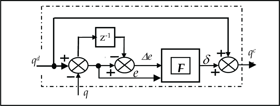
In order to compensate for losses, a fuzzy precompensator is integrated into the existing system. This is simply achieved by placing it in front of the SVM-inverse dynamics controller (Fig. 3). The fuzzy precompensator compensates for dynamic changes in the system and unpredictable external disturbances. It helps the inverse dynamics controller to provide the necessary actions that allow the end effector track the desired trajectory with minimum errors. The block diagram of the precompensator is shown in Fig. 4.

Figure 3.

SVM-based inverse dynamics control with a precompensator

Figure 4.

Fuzzy precompensator

The two inputs to the PD controller are e_i (k) and ė_i (k), where:

e_{i} (k) = q_{i}^{d} (k) - q_{i} (k), i = 1, \dots, n

(25)

is the trajectory tracking error vector and its first-order derivative is given by (26), where i refers to the i^−th joint and n to the number of joints.

{\dot{e}}_{i} (k) = q_{i}^{d} (k) - q_{i} (k), i = 1, \dots, n .

(26)

The output of the precompensator is considered now as the new reference input to the system; one can write:

q_{i}^{c} (k) = q_{i}^{d} (k) + δ_{i} (k), i = 1, \dots, n

(27)

The controller output δ_i (k) is generated by a nonlinear mapping function F implemented using fuzzy logic, such that:

δ (k) = F [e (k), Δ e (k)]

(28)

where:

\begin{array}{l} e_{i} (k) = q_{i}^{d} (k) - q_{i} (k) \\ Δ e_{i} (k) = e_{i} (k) - e_{i} (k - 1) ​ ​ ​ i = 1, \dots, n \end{array}

(29)

5.2 Stability Analysis

The presence of the fuzzy precompensator introduces a new joint position reference q^c, such that:

q^{c} = q^{d} + δ

(30)

In this case, (11) is rewritten as:

\overset{..}{e} + K_{v} \dot{e} + K_{p} e = Ψ \tilde{θ} + ν - u_{c}

(31)

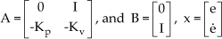
where ψ = M̆⁻¹Y, ν = M̆⁻¹ν′ and u_c = K_pδ. To study the stability of the tracking errors, we start by writing the system (31) in the state space:

\dot{x} = A x + B Ψ \tilde{θ} + B ν - B u_{c}

(32)

where Bν is a 2n×1 with an upper bound.

‖ B ν (t) ‖ < ν_{\max}

(33)

A is the Hurwitz matrix:

A = [\begin{matrix} 0 & I \\ - K_{p} & - K_{v} \end{matrix}], ​ ​ and ​ ​ B = [\begin{matrix} 0 \\ I \end{matrix}], x = [\begin{matrix} e \\ \dot{e} \end{matrix}]

In [27], it is seen that the adaptive control system designed for structured uncertainties will exhibit robustness in relation to bounded external disturbances. If we can compensate for the disturbing terms in equation (32), we may obtain disturbance rejection over the entire workspace of the robot manipulator. This can be done by synthesizing fuzzy control rules from human experts or using evolutionary algorithms. Our task is to guarantee the stability of the closed system in the sense that the state x remains uniformly bounded in face of parameter uncertainties and unknown disturbances. Looking at Fig. 4, the 2nx1 vector function approximator δ= F(e, Δe) is used to compensate any disturbances by providing the right amount of signal. Let us define the Lyapunov function candidate:

V = \frac{1}{2} x^{T} P x

(34)

where P is a symmetric positive definite matrix satisfying the Lyapunov equation:

A^{T} P + P A = - Q

(35)

for a given symmetric, positive definite matrix Q. Because A is stable, such P always exists. Using (32) and (35), the time derivative of V is obtained as:

\dot{V} = - \frac{1}{2} x^{T} Q x + x^{T} P B (Ψ \tilde{θ} + ν - u_{c}) \leq | x^{T} P B | (Ψ \tilde{θ} + ν - u_{c})

(36)

Our goal is to design u_c such that V̇ ≤ 0 - i.e., the controller u_c guarantees that |x| is decreasing. Therefore we should always have:

u_{c} \geq Ψ \tilde{θ} + ν

(37)

To implement this command online, the fuzzy precompensator should provide the quantity that should be added in such a way that constraint (37) is always satisfied. Therefore, the idea is to analyse the output response.

An increase in the command signal is needed whenever the error is around zero and the change-in-error is negative. Correspondingly, an increase in the command is necessary when we observe an increase in the error and the change-in-error. The other rules are obtained in a similar manner. For example, suppose that the error is zero and that the change-in-error is negative. This means that the output is increasing, heading in the direction of an overshoot. To compensate for this, we have to decrease the command signal. This corresponds to applying a correction term that is negative. The fuzzy precompensator is based on the Takagi-Sugeno type fuzzy model [30]. The realization of the function F[e(k),Δe(k)] obeys the procedures of fuzzification, fuzzy rule inference and defuzzification. Each membership function is a map from the universe of discourse to the interval [−1 1]. The Takagi-Sugeno's model is formulated following the form:

R_{ij} if e is A_{i}^{e} and Δe is A_{j}^{Δe} then δ_{ij} {=m}_{ij}; i=1, .. 7; j=1, .. 7 .

Where R_ij denotes the ij^−th implication and m_ij is the consequent parameter, A^e_i and A_j^Δe are fuzzy sets of the input membership functions. The output of the fuzzy precompensator is performed by the height defuzzification method, given the input pair (e_i(k), Δ_ej(k)); the final output is:

δ (k) = C_{F} \frac{\sum_{i = 1}^{49} μ (ς_{i}) ς_{i}}{\sum_{i = 1}^{49} μ (ς_{i})}

(38)

where ς_i is the support value at which the membership function reaches the maximum value and δ(k) is the consequent of the i^−th implication; the weight μ(ς_i), implies the overall truth of the premise of the i^−th implication, calculated as:

μ (ς_{i}) = A_{i}^{e} • A_{j}^{Δ e}

(39)

C_F is a scaling factor, defined for the three universes of discourse and whose values are chosen as: C_Fe=3.15; C_FΔe=5; C_Fy=10.0. The main difficulty in designing a fuzzy logic controller is the efficient formulation of the fuzzy If-Then rules. It is well-known that if it is easy to produce the antecedent parts of a fuzzy control rule, it will be difficult to produce the consequent parts of the rules without expert knowledge. The derivation of such rules is often based on the experience of skilled operators, the use of heuristic thinking [31, 32] or by modelling an expert's action [33].

6. Evolutionary Programming

In recent years, due to the availability of powerful computer platforms, the theory of evolutionary algorithms gained popularity to the problem of parameter optimization, although its origins can be traced back to the 1960s. They represent a well known family of optimization methods that have proven very attractive both for their stability and their effectiveness. These techniques have been exploited successfully in a broad range of applications including, for instance, biology, chemistry, control systems and image processing. This method is regarded as a parallel global search technique evaluating many points in the parameter space and it is more likely to converge towards a global solution. These algorithms perform a search by evolving a population of candidate individuals modelled with “chromosomes”. From one generation to the next, the population (set of candidate individuals) is improved by mechanisms inspired by genetics - i.e., through the use of both deterministic and nondeterministic genetic operators. Evolutionary programming (EP) is used to obtain the optimal consequent parts of the fuzzy precompensator rules.

6.1 Representation

Each individual chromosome represents a complete rule-base solution. The components (a₁ = m₁, a₂ = m₂, …, a_L = m_L) determine the consequent parts of the fuzzy rules, and the remaining components (a_L+1 = σ₁, a_L+2 = σ₂, …, a_2L = σ_L) contain standard deviations which control the mutation process. A complete string of chromosomes could be written in the following way, with a₁a₂ … a_La_L+1 a_L+2 … a_2L, representing one individual. The set of all the individuals represents a population. If we denote by P(t) a population at a time t, then we can write:

P (t) = {I^{1} (t), ​ I^{2} (t), ​ … ​, I^{μ} (t)}

(40)

where:

I^{i} = {a_{j}^{i}, ​ i = 1, …, μ; ​ j = 1, …, 2 L}

(41)

Iⁱ designates the i^−th individual in which aj describes the j^−th consequent part and the standard deviations, as was defined above. The algorithm seeks many local optima and increases the likelihood of finding the global optimum representing the problem goal.

6.2 Initialization

The algorithm is initiated by designating an initial population formed by 20 identical individuals. The number 20 is only an experiment number. Each solution is taken as a pair of real-valued vectors ( ${\vec{m}}_{i} , σ_{i}$ ), such that dim( ${\vec{m}}_{i}$ )=dim( ${\vec{σ}}_{i}$ )=number of rules. ${\vec{m}}_{i}$ is the consequent part vector of the fuzzy If-Then rules and σrarr;_i is an adaptable standard deviation vector. Initially, chromosomes in the current population are selected for reproduction according to the roulette wheel spinning method [34]. The adaptable standard deviations σ_i have been assigned an ad hoc choice of σ_i = 0.05; i=1,…,49.

6.3 Evaluation

The fitness function is evaluated for each set of rules and based on the function chosen to be:

Φ_{F} = \frac{1 0^{9}}{P E . ​ T E}

(42)

where:

\begin{array}{l} P E = \sum_{t} \sum_{i = 1}^{2} {(θ_{i}^{d} (k) - θ_{i} (k))}^{2}, \\ T E = \sum_{t} \sum_{i = 1}^{2} | τ_{i}^{d} (k) - τ_{i} (k) |, \end{array}

6.4 Generation

Generation in EP differs from that in GAs. The variation operators such as crossover and mutation perform differently. In fact, one child from one parent is generated by adding a normally distributed random value with an expectation zero and a unity standard deviation [35] as:

{\vec{m}}_{n e w}^{i} (j) = {\vec{m}}_{o l d}^{i} (j) + {\vec{σ}}_{o l d}^{i} (j) . N_{j} (0, 1)

(43)

N_j(0,1) indicates that the random variable is sampled anew for each value of the counter j. The step size σ is controlled by equation (44). The parameters τ and τ′ are the learning rates and adopt the conventional values of ${(\sqrt{2 n})}^{- 1} a n d {(\sqrt{2 \sqrt{n}})}^{- 1}$ respectively where n is the total number of rules to be evolved (in our case, n=49).

σ_{n e w}^{i} (j) = σ_{o l d}^{i} (j) . e x p [τ' . N (0, 1) + τ . N_{j} (0, 1)]

(44)

To help the system operating in a convergence and a stable region, certain constraints are utilized that are derived when the following assumptions are made:

Assumption 1 : The action values within the upper triangle of Table.1, denoted by m^U, are constrained to take negative values. Here: m^U(j,k) ∈ [−2, 0];

Assumption 2 : The action values within the lower triangle of Table.1, denoted by m^L, are constrained to take positive values. Here: m^L(j,k) ∈ [0, 2];

Assumption 3 : The action values within the off-diagonal of the lower triangle of Table.1, denoted by m^U/L, are free to take either positive values or negative values, with the one in the middle of the table constrained to take a zero value. i.e.:

{\begin{array}{l} m^{U / L} (j, k) \in [- 2, ​ ​ ​ ​ ​ 2]; ​ ​ j \neq k \\ m^{U / L} (j, k) = 0.0; ​ ​ ​ ​ ​ ​ ​ ​ ​ ​ ​ j = k \end{array}

(45)

The values −2 and 2 are chosen as lower and upper limits, successively and arbitrarily. To explain the natural meaning of the above assumptions, it is necessary to establish the link that gives input and output values based either on experience, a system step response or phase plane trajectory, so as to form the rule base. For example, if the reference signal is kept constant while the error is positive and the error change is negative, this means that the output is increasing towards an overshoot. Therefore, the input to the system should correspond to a negative value. After creating the new generation, a fitness score is evaluated for each new member ${\vec{m}}_{i}$ .

6.5 Selection

The next generation is selected based solely on the fitness values of the individuals. The selection is conducted by taking a random uniform sample of individuals of a size equal to half the population size among that of all the parents and offspring. Each solution from offspring and parent individuals is evaluated against the “q” randomly chosen individuals. For each comparison, a “win” is assigned if an individual score is better than or equal to that of its opponent, and the 20 new individuals with the greatest number of wins are retained as parents for the next generation. Their associated adaptable standard deviations are included.

7. Computer Simulation and Comparison

For simulation and comparison and without lost of generalities, a two-link robot manipulator was used to analyse and test the performance of the proposed approach. The rigid manipulator was modelled as two rigid links of lengths l₁=0.432m and l₂=.0432m with corresponding masses m₁=15.91Kg and m₂=11.36 Kg.

The simulations were carried out using the fourth-order Runge-Kutta algorithm, with the step h=0.01. The objective is to track the desired joint trajectories chosen to be:

\begin{array}{l} q_{1} = 1 + 2 (s i n t + s i n 2 t) \\ q_{2} = 2 + c o s 4 t + c o s 6 t \end{array}

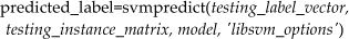
Two Matlab SVM libraries are used. The trainer SVM classifier, svmtrain, has the following syntax:

\begin{array}{l} model = svmtrain (t r a i n i n g_l a b e l_v e c t o r, t r a i n i n g_i n s t \\ a n c e_m a t r i x,' l i b s v m_o p t i o n s') \end{array}

(46)

and the prediction class of the new input data according to a pre-trained model, svmpredict, having the following syntax:

\begin{array}{l} predicted_label = svmpredict (t e s t i n g_l a b e l_v e c t o r, \\ t e s t i n g_i n s t a n c e_m a t r i x, m o d e l,' l i b s v m_o p t i o n s') \end{array}

(47)

During the training phase, we used a 3-fold CV, whereas the values of C and γ are found to be (8192, 0.25), (2048, 0.25), (5064, 0.25) and (1991, 0.25) for the four models M̆₁, M̆₂, V̆₁ and V̆₂ respectively. It is worth mentioning that the quality of SVM models depends on the proper settings of the SVMs' meta-parameters. However, there is no consensus on a given method for the choice of these parameters. In our case, the parameters are determined by a simple loop using a prepared Matlab script, summarized by the following algorithm:

Start Step 1) Set initial values for best_rate, best_C, and best_γ. Step 2) Set the initial value and the final value of cost C Step 3) Set the initial value and the final value of γ in the kernel function Step 4) Train an SVM classifier on the feature Space and assign the result to rate equ. (46) Step 5) If the rate is greater than or equal to best_rate, set best_rate as equal to rate, best_C as equal to C and best_γ as equal to γ. Step 6) Increment γ by some amount Step 7) If γ is not equal to γ_final,go to step 4 Step 8) Increment C by some amount Step 9) If C is not equal to C_final, go to step 4 End

The ε value of the intensive tube was fixed to 10⁻³. On the other hand, the rule base of the fuzzy precompensator is found by running the evolutionary algorithm with a population of 20 for about 500 generations. The resultant rule-base is depicted in Table 1.

Table 1.

Fuzzy logic rules for the precompensator.

First, the classical computed torque controller is implemented. As stated before, the values of the gains K_p and K_v can be adjusted so that the eigenvalues of the system in equation (9) assume the values that result in the acceptable responses of the system states.

To have an idea of the precision of the system, we propose to evaluate the proposed scheme in terms of the rising time and the settling time. We tested the position control in terms of RMS values, given by equation (48), when the first joint is made to move from 0 to (π/4) and the second joint from 0 to (−π/4).

RMSE = \sqrt{\frac{1}{n} \sum_{i = 1}^{n} e_{i}^{2}}

(48)

The simulation is carried out for the three cases for a lap of time equal to 1.12 sec. We report in Table 2 the results of the simulations, from where it is clear that the SVM precompensated system based on computed torque provides better results compared to the computed torque and the computed torque-based SVM approaches. Moreover, we show in Figs. 5, 6 and 7 the input step responses when the two links are moving in opposite directions. One can see the better performances observed on the computed torque-based SVM reinforced by the fuzzy precompensator (Figs. 7). The robustness of the last controller is obvious compared with the other two controllers when unknown payloads are added. In fact, this controller succeeded in rejecting the perturbation and maintaining its desired step response. On the other hand, the other two controllers show mediocre performances when the plant is perturbed, and the outputs move away from their desired step responses (Figs. 5 and Figs. 6).

Table 2.

Values of the position tracking error as RMSE.

RMSE	Joint (i)
RMSE	1	2
Computed torque	0.1941	0.2123
Computed torque based SVM	0.2031	0.2401
Computed torque based SVM precompensated	0.0557	0.1020

Figure 5(a).

Position tracking error of the 1^st joint (computed torque).

Figure 5(b).

Position tracking error of the 2^nd joint (computed torque).

Figure 6(a).

Position tracking error of the 1^st joint (SVM-computed torque).

Figure 6(b).

Position tracking error of the 2^nd joint (SVM-computed torque).

Figure 7(a).

Position tracking error of the 1^st joint (SVM-computed torque-precompensated).

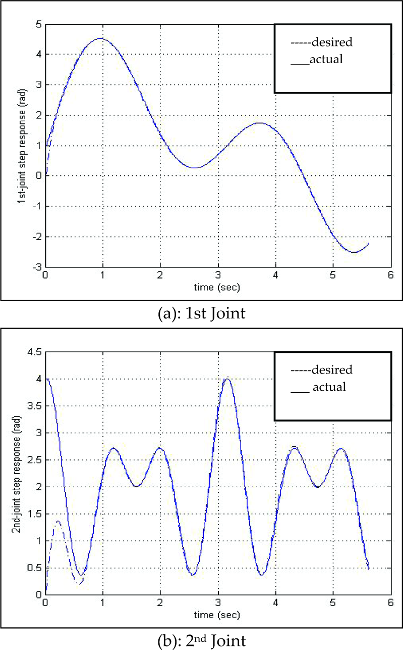
On the other, and for better illustration, we have plotted the desired and measured trajectories to show the tracking performances of the three techniques without perturbation (Figs. 8, 9 and 10). One can see that the tracking performances are excellent, since nonlinearities are cancelled.

Figure 7(b).

Position tracking error of the 2^nd joint (SVM-computed torque-precompensated).

Figure 8.

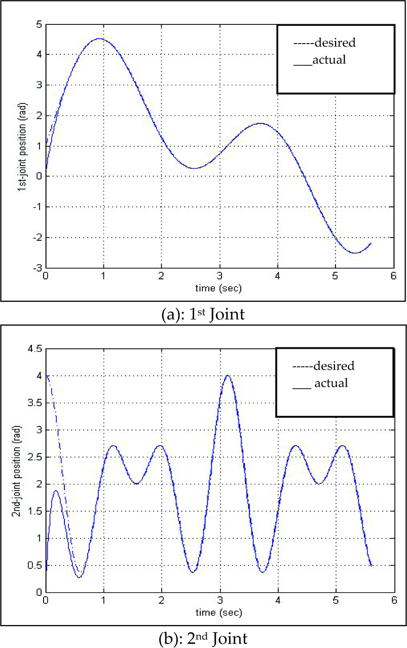
Trajectory tracking without perturbation, computed torque

Figure 9.

Trajectory tracking without perturbation, computed torque-based SVM

The trajectory tracking obtained using the SVM regressor-based inverse dynamic control which shows excellent tracking and a surprisingly better curve response in the transient part of the first joint - as can be seen in Fig. 9 - as determined by the accuracy of the regression model. These results illustrate the good performance of the SVM regression algorithm in approximating nonlinear functions and does not care about errors so long as they are less than ε, but will not accept any deviation larger than this.

The transient responses for the two joints are further improved (Figs. 10) when inserting the fuzzy precompensator in the previous configuration. In fact, the fuzzy precompensator is designed such that the inputs act like input reinforcement having the amount that must be added to the process input to compensate for current poor performances.

Figure 10.

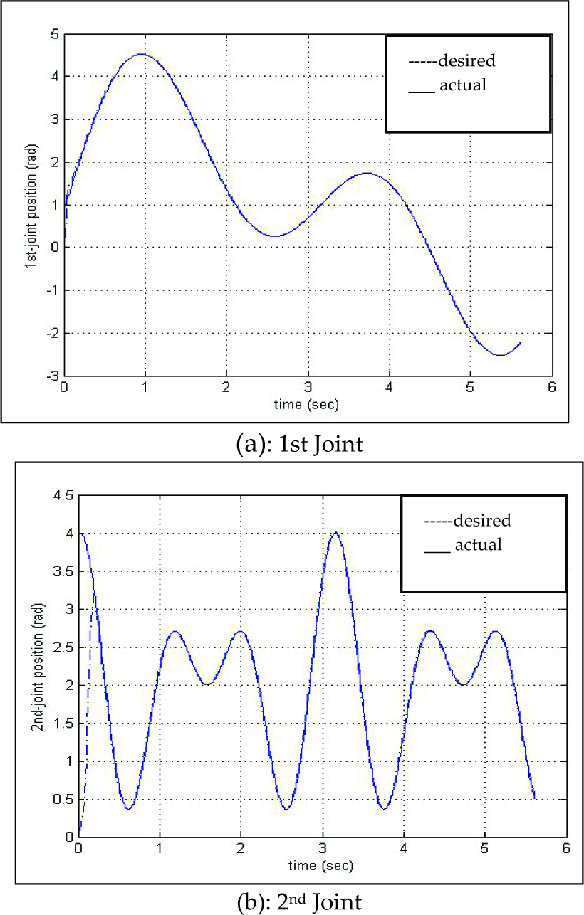
Trajectory tracking without perturbation, computed torque-based SVM precompensated.

To see the precision performance when perturbations are added, simulations were carried out by suddenly doubling the mass of the second link at time 2.5 sec and changing the values of both the viscous and Coulomb friction coefficients at the learning stage. In this case, the precision is relatively degraded for the computed torque method because the original design is perturbed and the parameters of the PD controller need to be updated to new values (cf. Figs. 11).

Figure 11.

Trajectory tracking with perturbation, computed torque

However, for the SVM regressor-based inverse dynamic control, the error tolerance seems to be much better for the two joints (Figs. 12). We explain this fact by the concept that states that the complexity of the model's representation by support vectors is independent of the dimensionality of the input space, depending instead only upon the number of support vectors.

Figure 12.

Trajectory tracking with perturbation, computed torque-based SVM.

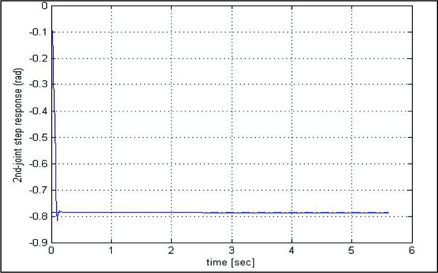
Now, to further improve the performance of the above approach and achieve global asymptotical tracking with fast transient responses and disturbance rejection, we activate the precompensator in the controlled system. In this case, the system can track the reference input much better despite any disturbances, as shown by Fig. 13. The evolution of joint position errors are depicted in Figs. 14, 15 and 16. They illustrate the tracking performances experienced by each method. One can note that in the absence of perturbations, the performances are almost the same. However, in presence of perturbation, the tracking performances are degraded for the computed torque and the SVM-based inverse dynamic, but remain adequate for the SVM-based inverse dynamics reinforced with the fuzzy precompensator, as is depicted in Figs. 17, 18 and 19 respectively. In fact, with the third scheme the maximum position errors are effectively decreased. This could be explained by the ability of the fuzzy precompensator to work around the goal positions, even though the PD controller parameters need not to be well tuned.

Figure 13.

Trajectory tracking with perturbation, computed torque-based SVM precompensated, -

Figure 14.

Performance of the computed torque control without perturbation

Figure 15.

Performance of the SVM-based inverse dynamic control without perturbation

Figure 16.

Performance of the SVM-based inverse dynamic reinforced with precompensator without perturbation

Figure 17.

Performance of the computed torque control with perturbation

Figure 18.

Performance of the SVM-based inverse dynamic control with perturbation

Figure 19.

Performance of the SVM-based inverse dynamic reinforced with precompensator with perturbation

On the other hand, the quality of tracking can be measured in terms of the normalized mean square error, defined as the Mean squared error/variance of the target, given by expression (49) as:

nMSE = \frac{\sum_{i = 1}^{N} {(f (x_{i}) - \overset{⌢}{f} (x_{i}))}^{2}}{\sum_{i = 1}^{N} {(f (x_{i}) - \bar{f} (x_{i}))}^{2}}

(49)

where:

\bar{f} (x_{i}) = \frac{1}{N} \sum_{i = 1}^{N} f (x_{i})

and N is the number of samples.

Table 3 gives the normalized squared error (nMSE) of the three studied methods when no perturbation is considered. When analyzing the results obtained, we come to the conclusion that the proposed novel approach attained excellent performances and that it is not contingent upon any assumptions related to the actual system. Comparing control quality using the three methods, the nMSE of the modelled system is mostly the same as the real system, due to better approximation.

Table 3.

Tracking error as the nMSE for each joint using reference trajectories without perturbation

nMSE	Joint (i)
nMSE	1	2
Computed torque	0.0027	0.2810
Computed torque-based SVM	0.0021	0.3662
Computed torque-based SVM precompensated	0.0012	0.3469

Using the required stored torques, we can solve for the time-consuming torque calculation, for which the values have to be provided as fast as the servo-loop. The role of the fuzzy precompensator is obvious through the results obtained in Table 4, which shows the performances achieved by this controller when the system is perturbed.

Table 4.

Tracking error as the nMSE for each joint using reference trajectories with perturbation.

nMSE	Joint (i)
nMSE	1	2
Computed torque	0.0028	0.2831
Computed torque-based SVM	0.0019	0.3213
Computed torque-based SVM precompensated	0.0009	0.2826

It is also important to have an idea of the effort developed on the joints. If we assume that each joint is driven by a DC motor via a transmission gear system, the control inputs are obtained in terms of voltage by multiplying the calculated torques by N⁻¹K_m⁻¹, where N represents the gear ratio and K_m is the torque constant, such that:

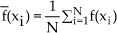
N₁ =120 for the first DC motor N₂ = 50 for the second DC motor K_m1=K_m2=0.18 Nm/Volt torque constant

We report on Figs. 20, 21 and 22 the curves of the control inputs when the robot manipulator evolves over the entire workspace without perturbations. On the other hand, we depict in Figs. 23, 24 and 25 the curves of the control inputs when the robot manipulator is perturbed by doubling the mass of the second link. The comparison between the Figures shows that the controller has compensated for the mass disturbance by an increase demand in energy. There is no doubt that the results obtained by the SVM-based computed torque controller enhanced with the fuzzy precompensator are highly satisfactory, as is clear from Figs. 22 and 25. The demand in energy to conduct the experiment with this controller is much less than that of its predecessors. Moreover, one can reduce any initial chattering by carefully tuning the scaling factor C_F in (37) or by choosing small initial amplitude responses. Comparing the three approaches, we come to the conclusion that the proposed scheme has the significant advantage in improving performance relative to the computed torque or the fixed gain controller. The simulation results showed that the computed torque based on SVM learning is a very interesting approach when a precise model of the robot manipulator is unknown or when the system is confronted with disturbances and uncertainties. SVM-based computed torque can achieve a relative low tracking error. In cases where high performances are needed, we can always support SVM-based computed torque with a fuzzy precompensator, which provides the amount needed by the plant when variations in the load or changes in the parameters of the plant are observed.

Figure 20.

Control effort for both joints without perturbation (computed torque)

Figure 21.

Control effort for both joints without perturbation (SVM-based inverse dynamic)

Figure 22.

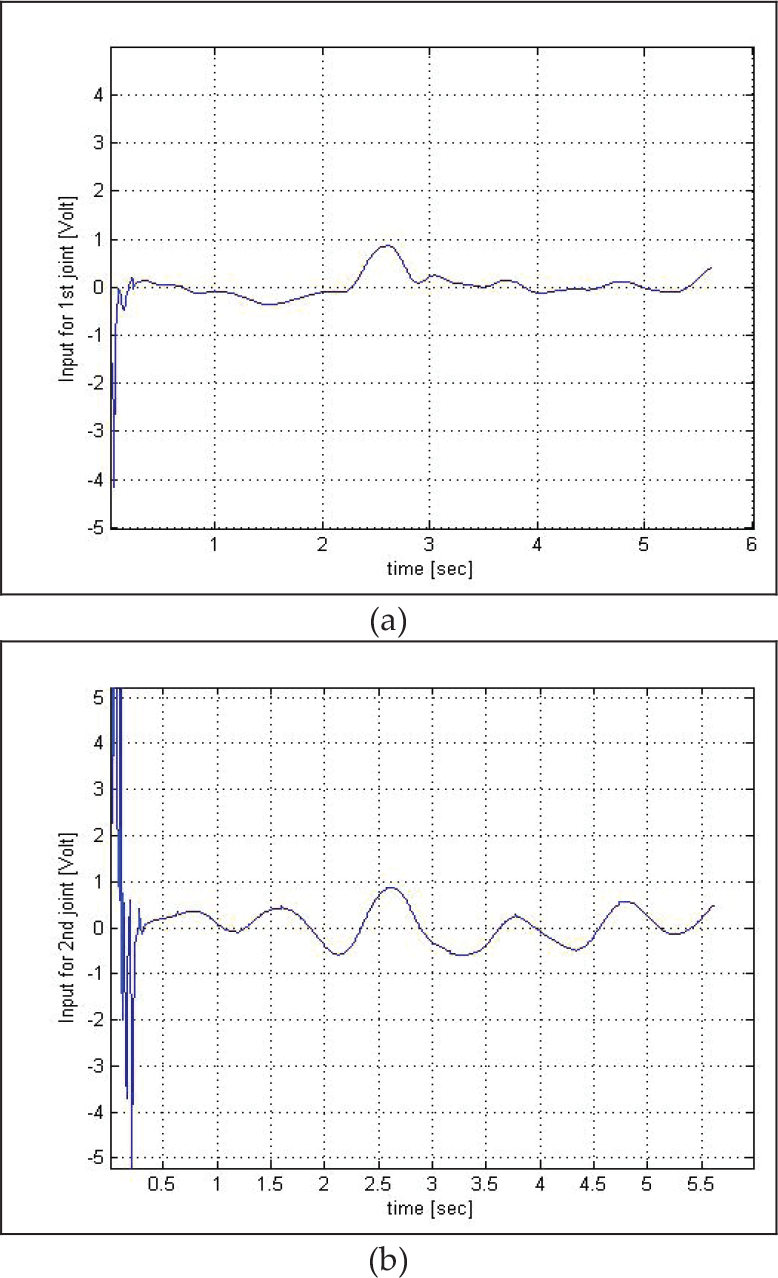
Control effort for both joints without perturbation (SVM-based inverse dynamic with precompensator)

Figure 23.

Control effort for both joints with perturbation (computed torque)

Figure 24.

Control effort for both joints with perturbation (SVM-based inverse dynamic)

Figure 25.

Control effort for both joints with perturbation (SVM-based inverse dynamic with precompensator)

8. Conclusion

In this paper, we propose a novel approach to nonlinear system control based on model dynamic compensation using one type of regressor brought from machine learning concepts, reinforced by a fuzzy precompensator. The idea is based on the computed torque method, which has been one of the successful tools used to control robot manipulators, since it eliminates the nonlinear parts of the system allowing the mechanical system to be controlled solely by a servo feedback PD controller. Unfortunately, the computed torque method gives rise to some drawbacks due to uncertainties in parameters and unforeseen perturbations. In this work, we propose a kernel regressor which is used to predict the feedforward torques when the desired trajectories are given. The learning is done offline and the results are most likely comparable to the computed torque method. The introduction of the fuzzy precompensator within the controlled system demonstrated improved performances due to fast transient responses and disturbance rejection. For the purpose of comparison, we included in the simulation results obtained by the computed torque control method. The simulation results show a better tracking trajectory, achieved by the SVM-based inverse dynamics control whenever any variation in the parameters occurred. Disturbance rejection and sensitivity were further improved when we inserted the fuzzy precompensator as part of the controller in order to reinforce the previous actions. All the simulation results were presented to demonstrate and prove the simplicity and the applicability of the SVM regression approach reinforced by a fuzzy precompensator to stabilize the robot manipulator with reduced steady-state error and less demand on effort.

Footnotes

9. Acknowledgments

This work was supported by the NPST programme of King Saud University, Project No: 08-ELE-300-02.

References

Craig

, “Introduction to Robotics: Mechanics and Control,” 3rd ed. Prentice Hall, 2004.

Vázquez

J. A.

and Velasco-Villa

, “Computed-Torque Control of an Omnidirectional Mobile Robot,” the 4th IEEE Int. Conf. on Electrical and Electronics Engineering (ICEEE), Mexico, pp. 274–277 Sep. 2007.

Cheah

C.C.

Hirano

Kawamura

and Arimoto

, “Approximate Jacobian Control for Robots with Uncertain Kinematics and Dynamics,” IEEE Transactions on Robotics and Automation, Vol. 19, No. 4, pp. 692–702, 2003.

Cheah

C.C.

Liu

and Slotine

J. J. E

, “Approximate Jacobian Adaptive Control for Robot Manipulators,” Proceeding of the IEEE International conference on Robotics and Automation, New Orleans, LA, pp. 3075–3080, 2004.

Raafat

S.M.

Said

W.K.

Akmeliawati

and Trik

N.M.

, “ Improving Trajectory Tracking for a Three axis SCARA Robot Using neural Network,” Symposium on Industrial Electronics & Application (ISIEA), Kuala Lumpur, Malaysia, Oct. 2009.

S.S.

Lee

T.H.

Harric

C.J.

, “Adaptive Neural Network Control of Robotic Manipulators”, World Scientific, London, 1998.

Ang

M.H.

Jr and Krishan

, “Neural Network Controller for Constrained Robot Manipulator,” In. Proc. IEEE Int. Conf. on Robotic and Automation, San Francisco, CA 1906–1911, 2000.

Shafiei

S. E.

and Soltanpour

M. R.

, “Robust Neural Network Control of Electrically Driven Manipulator Using Backstepping Approach”, International Journal of Advanced Robotic Systems, Vol. 6, No. 4, 2009.

Liu

, “Stability Analysis of Decentralized Adaptive Fuzzy Logic Control for Robot Arm Tracking,” proceeding of the 39^th IEEE conference on decision and control, Sydney, Australia, Dec. 2000.

10.

Yaochu

, “Decentralized Adaptive Fuzzy Control of Robot Manipulators,” IEEE Trans. On Syst Man, and Cyber.—Part B, Vol. 28, No. 1, Feb. 1998.

11.

Prabu

Kumert

and Prasad

“Advanced Dynamic Path Control of the Three Links SCARA Using Adaptive Neuro-Fuzzy Inference System”, Robot Manipulators, Trends and Development, ed. INTECH, pp. 336–359, 2010. ISBN 978-953-7619.

12.

Abdessemed

and Benmahammed

, “A Two-Layer Robot Controller Design Using Evolutionary Algorithms,” Journal of Intelligent and Robotic System, Vol. 30, pp. 73–94, 2001.

13.

Vapnik

V.N.

, “Statistical Learning Theory,” New York: John Wiley & Sons, 1998.

14.

Pontil

and Verri

, “Support Vector Machines for 3D Object Recognition,” IEEE Trans. on Pattern Analysis and Machine Intelligence, Vol. 20, pp. 637–646, 1998.

15.

El-Naqa Yongyi

Wernick

M.N.

Galatsanos

N.P.

, and Nishikawa

R.M.

“A Support Vector Machine Approach for Detection of Microcalcifications,”

IEEE Trans. on Medical Imaging, Vol. 21, pp. 1552–1563, 2002.

16.

Robinson

and Kecman

, “Combining Support Vector Machine Learning with the Discrete Cosine Transform in Image Compression,” IEEE Trans. on Neural Networks, Vol. 14, pp. 950–958, 2003.

17.

Bazi

and Melgani

“Toward an Optimal SVM Classification System for Hyperspectral Remote Sensing Images,”

IEEE Trans. Geosci. Remote Sensing, Vol. 44, pp. 3374–3385, 2006.

18.

Lei

Song

Qiu

and Ge

, “Application of SVM in Intelligent Robot Information Acquisition and processing: A survey,” Int. Conf. on Information Acquisition, Hong Kong (China), pp. 175–180, 2005.

19.

Nguyen-Tuong

Seeger

and Peters

, “Computed Torque Control with Nonparametric Regression Models,” American Control Conf., pp. 212–217, June 2008.

20.

Cheah

C.C.

Liu

and Slotine

J.J.E

, “Adaptive Tracking Control for Robot with Unknown Kinematic and Dynamic Properties,” The Int. Journal of Robotic Research, Vol. 25, No. 3, pp. 283–296, 2006.

21.

Abdessemed

and Baazi

, “SVM-Based Computed Torque for Robot Manipulator Control”, Conf. on Methods and Models in Automation and Robotics MMAR 2009.

22.

Smola

and Schölkopf

, “A Tutorial on Support Vector Regression,” Tech. Report, Royal Holloway College, Univ. London, U.K., NeuroCOLT. NC-TR-1998-030, Oct. 1998.

23.

Kwok

J.T.

, “Linear Dependency Between ε and the Input Noise in ε-Support Vector Regression,” in: Dorffner

Bishop

, and Honik

(Eds): ICANN, LNCS 2130, pp. 405–410, 2001.

24.

Smola

Murata

Schölkopf

and Muller

, “Asymptotically Optimal Choice of ε-loss for Support Vector Machines,” Proc. ICANN, 1998.

25.

Scholkopf

Bartlett

Smola

and Williamson

, “Support Vector Regression with Automatic Accuracy Control,” Proceedings of the 8-th Int. Conf. on Artif. Neural Net., Perspectives in Neural Computing, Berlin: Springer, Verlag, 1998.

26.

Schölkopf

Smola

and Müller

K.R.

, “Nonlinear Component Analysis as a Kernel Eigenvalue Problem,” Neural Computation, Vol. 10, pp. 1299–1319, 1998.

27.

Cristianini

and Shawe-Taylor

, “An Introduction to Support Vector Machines and Other Kernel-based Learning Methods,” Cambridge University Press, 2000

28.

Stone

, “Cross-Validatory Choice and Assessment of Statistical Predictions,” Jour. R. Statist. Soc. B, Vol. 36, No. 1, pp. 111–147, 1974.

29.

Craig

J.J.

Hsu

and Sastry

S.S.

, “Adaptive Control of Mechanical Manipulators,” The Int. Journal of Robotics Research, Vol. 6, No. 2, pp 16–28, 1987.

30.

Sugeno

, “Industrial Application of Fuzzy Control,” Elsevier science publisher B. V-Netherlands, 1985.

31.

Tay

. and Tan

S.W.

, “Fuzzy Systems as Parameter Estimator of Nonlinear Dynamic Function,” IEEE, Trans Syst, Man, Cybern- Part B, Vol. 27, No. 2, 1997.

32.

Wang

L.X.

, “Stable adaptive fuzzy control of nonlinear systems,” IEEE Trans. on Fuzzy Systems, Vol. 1, No. 2, 1993.

33.

Abe

and Lan

M.S.

, “A method for fuzzy rules extraction directly from numerical data and its application to pattern classification,” IEEE Trans. Fuzzy Systems, Vol. 3, pp. 18–28. 1995.

34.

Goldberg

D.E.

, “Genetic Algorithms in Search, Optimization and Machine Learning,” Addison-Wesley, Reading, MA, 1989.

35.

Bach

Hammel

and Schwefel

H.P.

, “Evolutionnary Computation: Comments on the History and Current State,” IEEE Trans. Evolutionary Computation, Vol. 1, 1997.

SVM-Based Control System for a Robot Manipulator

Abstract

Keywords

1. Introduction

2. Problem formulation

3. Inverse Dynamics Control

4. Support Vector Regression and Model Estimation

4.1 Regression with the SVM

4.2 Robot Model Estimation with Support Vector Regression

4.3 Discussion

5. The Fuzzy Precompensator

5.1 Analysis and Design

5.2 Stability Analysis

6. Evolutionary Programming

6.1 Representation

6.2 Initialization

6.3 Evaluation

6.4 Generation

6.5 Selection

7. Computer Simulation and Comparison

8. Conclusion

Footnotes

9. Acknowledgments

References