Sage Journals: Discover world-class research

Abstract

Optimal path-planning for mobile robot recharging is a very vital requirement in real applications. This paper proposes a strategy of determining an optimal return-path in consideration of road attributes which include length, surface roughness, road grade and the setting of speed-control hump. The road in the environment is partitioned into multiple segments, and for each one, a model of cost that the robot will pay for is established under the constraints of the attributes. The cost consists of energy consumption and the influence of vibration on mobile robot that is induced by motion. The return-path is constituted by multiple segments and its cost is defined to be the sum of the cost of each segment. The idle time, deduced from the cost, is firstly used as the decision factor for determining the optimal return-path. Finally, the simulation is given and the results prove the effectiveness and superiority of the strategy.

Keywords

Mobile robot recharging Road attribute Surface roughness Road grade Idle time.

1. Introduction

Autonomous mobile robots have been developed to perform numerous routine tasks, such as automatic patrolling in a transformer substation [1], transporting in a warehouse [2] and guiding working in a museum [3]. Each application desires the autonomous mobile robots smart enough to survive in its environment without operator intervention. Energy is of crucial concern, and without it the robot will become immobilized and useless [4, 5]. Typically, rechargeable batteries may only provide a few hours of peak usage for the robot once, for example, with a battery pack, a Honda humanoid robot can run for only 30 mins [6]. As a result, to achieve true long-term autonomy, the robot must find a charging station and recharge itself before the power of the batteries is exhausted [7]. Therefore, the important issue of optimal path planning on energy-minimizing attracts considerable attentions continuously.

In indoor environment or square of fine surface, usually the amount of energy consumption is approximately proportional to the length of path that the robot has passed. Hence, for simplicity, some researchers plan to search the shortest obstacle-avoiding paths, which are recognized as the optimal paths [8 –12]. However, in outdoor environments, the criterion of the shortest-length may no longer be suitable because motion of the robots is highly influenced by terrain characteristics [13, 14]. There are few existing methods for field robot navigation that consider this restraint and other criterions such as minimum-time and minimum energy cost are adopted [15 –19]. In [18], a number of constraints such as impermissible traversal directions are employed since the environment aimed at is the huge wild area (e.g., a river basin referred in the article). It is thus inevitable to cause the complexity of computing. In the studies on minimum weighted paths planning [15, 16, 19], the weight (e.g., the cost of time or energy consumption) is used as a parameter for theoretical analysis, but no detail of the derivation of the relation between the weight and the road attributes is involved. Additionally, the problem of minimum-time path planning in a 2-1/2-D environment is investigated [17]. However, the assumption is that the robot is working with maximum power, and then time is used as the decision factor for optimal path determination. It is worth mentioning that, Guo et al. adopt the terrain roughness and terrain slope to define the power consumption. However, although it has qualitative analysis, no experiment is executed for quantitative analysis [20]. Besides, Mei et al. discuss the most energy-efficient path planning [13]. However, it focuses on the discussion about energy spent on robot's turning and rotating, while the terrain characteristics are not mentioned.

Furthermore, the dynamic and kinematic constraints are also considered in motion plan. For example, for arbitrarily contoured terrain such as hilly terrain, the anisotropic friction, gravity effects and ranges of impermissible-traversal headings are discussed for overturn danger or power limitation [21]. The dynamic and wheel/ground interaction constraints are dealt with in the motion planning for all-terrain robots, where the environment is thought to be composed of a set of static obstacles, sticky areas and slippery regions [22]. In [20], Guo et al. propose path planning and control of noholonomic mobile robots in rough terrain environments, where performance issues including robot safety, geometric, time-based and physics-based criteria are refereed. In addition, Kobilarov et al. present a planner that finds near optimal trajectories on outdoor terrain based on control-driven probabilistic road maps [23]. They consider the safety of the robot and use an upper bound on the maximum pitch of the robot. All these indicate that the influence of motion on robot should not be neglected in outdoor environment. Nevertheless, in the majority of the studies currently presented in the literature, the terrain characteristics are just considered as constraints for various purposes in path planning, but without quantitative analysis. Moreover, researches have tried to classify the terrain based on vibrations induced by wheel-terrain interaction [24, 25]. Different terrain surfaces have different influence on robot, but the authors did not show the impact on the robot in practical application.

As the improvement and synthesis, in our approach of determining the optimal return-path, we take into account both energy consumption and the quantitative analysis on the influence of vibration on mobile robot. Generally, once energy consumption occurs, the robot will spend some time on recharging to compensate the loss, and the time here, is called the idle time which means non-working time. Similarly, the time spent on repairing the robot belongs to the idle time too. Usually, it might take several hours or more to check and repair once the robot is found in abnormal operation state. The reason for repairing is mainly the continuous vibration which may loose the connections among equipments of the robot. And the vibration will exist as long as the robot is walking. Naturally, if the total idle time is minimized, then the working time will be maximized. Hence, we plan to determine an optimal return-path with minimum idle time. To our knowledge, it is the first time to use idle time as the decision factor, which is proved to be more effective for evaluating paths.

This paper is organized as follows: this section has summarized related work and proposed our strategy. In Sect. 2 the research problem and motivation are stated. In Sect. 3 the models of working environment and road attributes are described. In Sect. 4 we address the implementation of the strategy proposed. In Sect. 5 simulation and results are provided as well as discussions. Finally, conclusion is made and further study is announced.

2. Problem Statement and Motivation

In outdoor environment, some special scenarios should be emphasized, e.g., the situations shown in Fig. 1.

Figure 1.

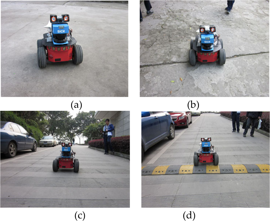
Four typical situations in practice: a robot is (a) walking on a flat road; (b) walking on a rough road; (c) walking on a slope and (d) passing a speed-control hump.

In Fig. 1(a), a robot is walking on a path having plain surface while in Fig. 1(b), it is walking on a road of rough surface. In Fig. 1(c) the robot is going straight downhill on a slope and in Fig. 1(d) it is passing a speed-control hump. These reveal the diverse situations in outdoor environment. Because of these various features, the following phenomena will inevitably occur: (i) the bad influence of vibration on equipments is bigger when the robot runs on a rough road compared to a plain one, and more energy consumption rate is destined since of the bigger surface resistance [26]; (ii) on the same slope, different energy consumption rates occur since the robot may be going uphill or downhill; (iii) drastic vibration occurs while the robot is passing over a speed-control hump compared to walking on ordinary road surface. As a result, the same road or different roads with the same length may cost different energy consumption and have influences of different level on the robot's body.

The analysis above shows that path length will no longer be suitable for evaluating the paths in outdoor environment, since extra energy consumption rate and influence of vibration on robot exist. As mentioned in Sect. 1, this paper endeavors to determine the optimal path using the idle time as the decision factor. From a different angle, we say that less idle time means the prolonged working-time. This conforms to the target that maximizing the rate of working. Hence, the main task is to clarify how the road attributes are employed to analyze the impact on idle time.

In this paper, the road in the environment is divided into multiple segments, whose attributes can be pre-collected. We first find out each path accessible to a certain dock, and compute the cost by summing the costs of the multiple road segments consisting this path. The optimal return-path with minimum idle time will be selected out. Therefore, in this paper, great efforts are made to deduce the quantitative relation between the idle time and the multiple attributes of road.

3. The Model of Working Environment

This section establishes the model of working environment by using a metric topological map. First, some assumptions are made:

There has H docks placed in the environment, which are noted as D₀, D₁,…, D_h,…,D_H–1 respectively. For example, in Fig. 2, D_h is a dock.

The road is partitioned into M segments. Each segment P_m (m = 0,1,…, M −1) has four attributes: p_ml,p_mr,p_mg and p_mh, where p_ml (unit: m) represents the length of P_m,p_ml (unit: m/km) is the surface roughness, and p_mh implies how many speed-control humps are fixed on this segment. p_mg (unit: rad) is the actual road grade of P_m, and –π/2 < p_mg < π/2. The four properties can be understood more clearly by the profile of a segment shown in Fig. 3.

Figure 2.

The model of working environment. D_h is a dock, P_m shown as a green line is a road segment. Each blue line represents a speed-control hump. The shadow implies that it is a rough segment. The regions with oblique lines represent obstacles.

Figure 3.

The attributes p_ml,p_mr,p_mg and p_mh of a segment P_m.

Specifically, the sign of p_mg is decided by the coordinates of the two endpoints. In the coordinate system shown in Fig. 2, for P_m,A(x, y) represents one endpoint that has smaller abscissa value or smaller ordinate value and the same abscissa value with the other endpoint. We note the other point as B(x, y). According to Fig. 3, for P_m in Fig. 2, the sign of p_mg is decided by

{\begin{cases} p_{m g} \geq 0, A (x, y) corresponds    to A^{'} actually \\ p_{m g} < 0, A (x, y) corresponds    to B^{'} actually \end{cases}

(1)

Observed from (1), if p_mg > 0, the robot is uphill actually when going from A to B or else downhill.

The cost that the robot will pay for passing each segment includes two parts: energy consumption c_e and the influence of vibration on robot body c_b that describes the probability of robot's equipment failure. The cost C then can be described as

C = (c_{e}, c_{b})

(2)

4. The Implementation of the Strategy

In this section, the force analysis when the robot is walking on a road segment is carried out first, then the mathematical models of c_e and c_b are established based on the road attributes. At last the strategy of determining the optimal return-path is described in detail using c_e and c_b.

4.1 The Force Analysis of the Mobile Robot

A longitudinal robot model is built to analyze the forces shown in Fig. 4. The robot is constrained by five forces: the engine force F_engine, the rolling resistance F_roll, the brake force F_brake, the air drag F_air and the gravity induced force F_gravity respectively [27].

Figure 4.

Force analysis of the mobile robot when passing a road segment.

Given a robot walking at low speed and without braking, the impact of F_air and F_brake are omitted, then we obtain

{\begin{cases} F_{a i r} = 0 \\ F_{b r a k e} = 0 \end{cases}

(3)

With Fig. 4, F_roll can be expressed as

F_{r o l l} = γ_{r} m_{r} g \cos (p_{m g})

(4)

where γ_r is the coefficient of rolling resistance that is proportional to p_mr. Let ρ(ρ > 0) be the proportion, i.e., γ_r = ρρ_mr, then

F_{r o l l} = ρ p_{m r} m_{r} g \cos (p_{m g})

(5)

In addition, F_gravity is induced by gravity G, and the relationbetween F_gravity and p_mg is

F_{g r a v i t y} = m_{r} g \sin (p_{m g})

(6)

where m_r is the weight of the robot and g is the gravitational constant.

Assume that the robot walks at a constant velocity, that is to say, the acceleration is zero, and then with (3) we obtain

F_{e n g i n e} = F_{r o l l} + F_{g r a v i t y}

(7)

4.2 Computation of the Idle Time

This section will first deduce the mathematical models of c_e and c_b according to the attributes and force analysis above, and then based upon the models we compute the idle time.

4.2.1 Mathematical Model of c_e

Define $W_{p_{m l}}$ as the total work the robot does when moving for distance p_ml dragged by F_engine, and assume no energy consumption for making turns, then

W_{p_{m l}} = F_{e n g i n e} p_{m l}

(8)

According to (5), (6) and (7) additionally, we have

W_{p_{m l}} = ρ p_{m r} m_{r} g \cos (p_{m g}) p_{m l} + m_{r} g \sin (p_{m g}) p_{m l}

(9)

In this paper, the energy the robot needs to drive motors is supplied by batteries. We assume the energy consumption is proportional to the total work, i.e., $c_{e} \propto W_{p_{m l}}$ . Thus, we describe c_e using $W_{p_{m l}}$ and a positive coefficient λ as

c_{e} = λ W_{p_{m l}}

(10)

As c_e is the result of long-term accumulation of energy consumption, the energy spent on passing a single speed-control hump can be ignored. We define r_e (unit: V/m) as the energy consumption rate of walking on road, which means the average voltage decrease (unit: V) of passing per meter long road. Therefore, for passing a road segment P_m with attribute p_ml,c_e is calculated as

c_{e} = r_{e} p_{m l}

(11)

According to (9), (10) and (11), we get

r_{e} = ρ p_{m r} λ m_{r} g \cos (p_{m g}) + λ m_{r} g \sin (p_{m g})

(12)

Let κ; = λm_rg, then (12) becomes

r_{e} = κ ρ p_{m r} \cos (p_{m g}) + κ \sin (p_{m g})

(13)

We will discuss two situations in terms of p_mg and p_mr:

p_mg = 0 and p_mr = μ_f.

First, we consider that a road has attributes p_mg = 0 and p_mr = μ_f. According to (13), we obtain the energy consumption rate $r_{e_μ_{f}}$ of this situation:

r_{e_μ_{f}} = κ ρ μ_{f}

(14)

Define $r_{e_p_{m r}}$ as the energy consumption rate for passing any segment of p_mg = 0 and p_mr, then with (14) we have

r_{e_p_{m r}} = κ ρ p_{m r} = \frac{p_{m r}}{μ_{f}} r_{e_μ_{f}}

(15)

p_mg = ϕ_g (ϕ_g ≠ 0) and p_mr = μ_f.

Define $r_{e_μ_{f} ϕ_{g}}$ as the energy consumption for a segment having attributes p_mg = ϕ_g and p_mr = μ_f, then with (13) we have

r_{e_μ_{f} ϕ_{g}} = κ ρ μ_{f} \cos ϕ_{g} + κ \sin ϕ_{g}

(16)

then with (14) and (16), we have

κ \sin ϕ_{g} = r_{e_μ_{f} ϕ_{g}} - r_{e_μ_{f}} \cos ϕ_{g}

(17)

According to (13)–(17), for any segment having attributes p_mg and p_mr, we have

r_{e} = \frac{r_{e_μ_{f}}}{μ_{f}} p_{m r} \cos (p_{m g}) + \frac{r_{e_μ_{f} ϕ_{g}} - r_{e_μ_{f}} \cos ϕ_{g}}{\sin (ϕ_{g})} \sin (p_{m g})

(18)

With given values μ_f and ϕ_g, if $r_{e_μ_{f}}$ and $r_{e_μ_{f} ϕ_{g}}$ are measured experimentally, the energy consumption rate r_e for passing any segment P_m of attributes p_mg and p_mr can be obtained.

Let $Δ r_{e_r} = \frac{r_{e_μ_{f}}}{μ_{f}} and Δ r_{e_g} = \frac{r_{e_μ_{f} ϕ_{g}} - r_{e_μ_{f}} \cos ϕ_{g}}{\sin (ϕ_{g})}$ , (18)

Becomes

r_{e} = Δ r_{e_r} p_{m r} \cos (p_{m g}) + Δ r_{e_g} \sin (p_{m g})

(19)

With (11) and (19), the energy consumption c_e of passing P_m is obtained

c_{e} = (Δ r_{e_r} p_{m r} \cos (p_{m g}) + Δ r_{e_g} \sin (p_{m g})) p_{m l}

(20)

4.2.2 Mathematical Model of c_b

The vibration on robot is caused by lots of factors such as the nonlinearity of robot body, speed-control hump and the road surface roughness [26]. Here, we mainly focus on the latter two factors. Define c_{b_r} as the influence caused by passing road surface and r_{b_r} as the average influence of passing per meter long road, then

c_{b_r} = r_{b_r} p_{m l}

(21)

A system's reliability is usually indicated by the Mean Time Between Failures (MTBF). Here, we define the Mean Length Between Maintenances (MLBM) in a similar way to describe the quality of connections among devices in the robot. Here, MLBM implies the average length of path the robot has traveled between two successive maintenances. Hence, the practical meaning of r_{b_r} is the average probability value leading the robot to be repaired when the robot passes per meter long road with certain speed. We use L_MLBM (unit: m) to express the value of MLBM. Assume that L_MLBM is measured to be L m, i.e., L_MLBM = L m, then we obtain

r_{b_r} = \frac{1}{L_{M L B M}} = \frac{1}{L} m^{- 1}

(22)

If the average influence is measured to be $r_{b_μ_{f}}$ for P_m of given surface roughness p_mr = μ_f, then

r_{b_r} = \frac{p_{m r}}{μ_{f}} η r_{b_μ_{f}}

(23)

where η(η > 0) implicates the proportional relation between the influence degree and surface roughness.

For a slope, the extra influence caused by road grade is ignored since no extra vibration will occur compared with a road whose road grade is zero. Hence we set the extra influence of slope r_{b_s} to be zero, i.e., r_{b_s} = 0.

The speed-control humps will bring about vertical vibration with much bigger amplitude compared to road surface. Define r_{b_h} as the average probability causing the robot to be repaired while passing a speed-control hump, then the total influence c_{b_h} caused by speed-control humps in P_m is

c_{b_h} = p_{m h} r_{b_h}

(24)

With (21), (23) and (24), we obtain the cost c_b of P_m:

c_{b} = c_{b_r} + c_{b_h} = \frac{r_{b_μ_{f}}}{μ_{f}} η p_{m r} p_{m l} + p_{m h} r_{b_h}

(25)

4.2.3 Computing the Idle Time

The final purpose of various kinds of planners or optimizations is to maximize the working time. However, in this paper, we minimize the idle time (noted as T_IDLE) including recharging time T_C and repairing time T_R to achieve this purpose indirectly.

Define T_C (unit: s) as the time spent on recharging to compensate the energy consumption c_e, then

T_{C} = \frac{c_{e}}{v_{c h a r g e}}

(26)

where v_charge (unit: V/s) is the charging speed that can be derived by

v_{c h a r g e} = \frac{V_{f u l l} - V_{l o w}}{T_{C}}

(27)

where V_low and V_full are the initial voltage value and the eventual value after fully charged respectively. In practice, v_charge can be measured experimentally.

In engineering, the Mean Time To Repair (MTTR) is usually used to describe the resumption performance of production. Here, we describe the cost c_b using MTTR. Let T_MTTR represent the MTTR of our robot and note T_R (unit: s) as the repairing time induced by c_b then we have

T_{R} = c_{b} T_{M T T R}

(28)

Then T_idle is the sum of T_C and T_R, namely,

T_{I D L E} = T_{C} + T_{R} = \frac{c_{e}}{v_{c h a r g e}} + c_{b} T_{M T T R}

(29)

Since c_e and c_b are two elements of C, so, if we use function f (C) to describe the relation between T_IDLE and C, i.e.,

T_{I D L E} = f (C) = f (c_{e}, c_{b}) = \frac{c_{e}}{v_{c h a r g e}} + c_{b} T_{M T T R}

(30)

4.3 Determining the Optimal Return-path

Based on the mathematical model of c_e,c_b and T_IDLE, the details of the procedure of determining the optimal return-path are described:

Step 1: Find out all the accessible paths to dock D₀ from the current position where the robot begins to return. Calculate the cost and idle time for each return-path and figure out the optimal return-path to dock D₀.

Assume that there has N different return-paths accessible to dock D₀, which are noted as $R_{D_{0} 0}$ , $R_{D_{0} 1}$ ,…, $R_{D_{0} n}$ ,…, $R_{D_{0} (N - 1)}$ , and the costs are $C_{R_{D_{0} 0}}$ , $C_{R_{D_{0} 1}}$ ,…, $C_{R_{D_{0} n}}$ ,…, $C_{R_{D_{0} (N - 1)}}$ resepctively. Note that each return-path is constituted by a sequence of segments. As an example, for a certain $R_{D_{0} n}$ ( $n = 0, 1, …, N - 1$ ), assume that it is constituted by G (0 < G ≤ M) segments and the order is P₀, P₁,…, P_g,…,P_G–1, then we express $R_{D_{0} n}$ as

R_{D_{0} n} = {P_{0}, P_{1}, …, P_{g}, …, P_{G - 1}}

(31)

For a segment P_g (g = 0,1,…, G–1), we note its cost as

C_{P_{g}} = (c_{e_P_{g}}, c_{b_P_{g}})

(32)

Thus, $C_{R_{D_{0} n}}$ ( $n = 0, 1, …, N - 1$ ) is the sum of $C_{P_{g}}$ :

C_{R_{D_{0} n}} = (c_{e_R_{D_{0} n}}, c_{b_R_{D_{0} n}}) = (\sum_{g = 0}^{G - 1} c_{e_P_{g}}, \sum_{g = 0}^{G - 1} c_{b_P_{g}})

(33)

We use $T_{I D L E_R_{D_{0} n}}$ to describe the idle time caused by $R_{D_{0} n}$ , then according to (30) and (33), we have

T_{I D L E_R_{D_{0} n}} = f (C_{R_{D_{0} n}}) = f (\sum_{g = 0}^{G - 1} c_{e_P_{g}}, \sum_{g = 0}^{G - 1} c_{b_P_{g}})

(34)

After computing the idle for each return-path $R_{D_{0} n}$ , we select out the optimal one and note it as $R_{D_{0}}$ , The criterion of selection is

T_{I D L E_R_{D_{0}}} = m i n {T_{I D L E_R_{D_{0} n}} | n = 0, 1, …, N - 1}

(35)

where the decision function min that will appear in (36) and (37) again means selecting the one with minimum value.

Step2: Figure out the respective optimal return-path to each dock D_h (h = 0, 1,…, H −1).

After performing the same process for the h'th (h = 0, 1,…, H −1) dock, H −1 optimal return-paths to the other docks are derived, which are marked as $R_{D_{1}}$ , $R_{D_{2}}$ ,…, $R_{D_{h}}$ ,…, $R_{D_{H - 1}}$ . For each $R_{D_{h}}$ ( $h = 0, 1, …, H - 1$ ), we have

T_{I D L E_R_{D_{h}}} = m i n {T_{I D L E_R_{D_{h} n}} | n = 0, 1, …, N - 1}

(36)

Setp 3: From $R_{D_{0}}, R_{D_{1}}, \dots, R_{D_{h}}, \dots, R_{D_{H - 1}}$ , we determine the optimal return-path, and note it as $R_{D_{O P}}$ . This optimal return-path is what we want finally, and is selected by

T_{I D L E_R_{O P}} = m i n {T_{I D L E_R_{D_{h}}} | h = 0, 1, …, H - 1}

(37)

5. Simulation, Results and Discussions

This section will first determine the values of parameters by experiments, then the simulation, results and discussions will be presented.

5.1. Determination of the Values of Parameters Experimentally

Here we will compute the values of relevant parameters appeared in Sect. 3 and Sect. 4 through experiments.

$r_{e_μ_{f}}$ and $r_{e_μ_{f} ϕ_{g}}$ .

First, we measure the values of $r_{e_μ_{f}}$ and $r_{e_μ_{f} ϕ_{g}}$ appeared in (18) in Sect. 4.2 in order to compute r_e.

Assume that V_start is the voltage value when the robot begins to work, and V_end the value after running at the average speed $\overset{―}{v}$ for time $\overset{―}{t}$ , then r_e (unit: V/m) is calculated as

r_{e} = \frac{V_{s t a r t} - V_{e n d}}{\overset{―}{v} \overset{―}{t}}

(38)

Actually, some researches have tried to classify the terrain based on vibrations induced by wheel-terrain interaction [24]. Similarly, in this paper, observed from the real environment, the road surfaces are divided into two kinds, i.e., the flat surface and the rough surface, which are shown in Fig. 1(a) and Fig. 1(b) respectively. We use μ_f and μ_r to describe the surface roughness of these two typical roads respectively. The energy consumption rates $r_{e_μ_{f}}$ and $r_{e_μ_{f} ϕ_{g}}$ are estimated in the following.

A Pioneer3-AT robot produced by MobileRobot Inc. is utilized in the experiment [28]. Three lead acid cells are employed to provide energy for the robot, and the full voltage V_full; is observed to be 12.7V. In practice, to ensure that the robot has enough power to go to the nearest dock wherever it begins to return, the threshold voltage V_law warning the robot to return for recharging is set to be 11.3V. In the experiments, the robot starts to run at full voltage, and keeps running at the average speed of $\overset{―}{v} = 0.75 m / s$ till the voltage valye decreases to 11.3V. After testing many times on flat road of roughness μ_f, the average continuous running time $\overset{―}{t_{f}}$ is measured to be about 2.67 hours. Hence, $r_{e_μ_{f}}$ is derived:

r_{e_μ_{f}} = \frac{12.7 V - 11.3 V}{0.75 m / s \times 2.67 h \times 3600 s / h} \approx 0.1942 \times 10^{- 3} V / m

(39)

The same tests are repeated on a rough road of roughness μ_r, and we get $\overset{―}{t_{r}} \approx 2.07 h$ , therefore,

r_{e_μ_{r}} = \frac{12.7 V - 11.3 V}{0.75 m / s \times 2.07 h \times 3600 s / h} \approx 0.2505 \times 10^{- 3} V / m

(40)

Actually, according to (15), $r_{e_μ_{r}} = \frac{μ_{r}}{μ_{_{f}}} r_{e_μ_{f}}$ , Therefore, with (39) and (40), the relation between μ_f and μ_r is derived:

μ_{r} = \frac{r_{e_μ_{r}}}{r_{e_μ_{f}}} μ_{f} = \frac{0.2505 \times 10^{- 3}}{0.1942 \times 10^{- 3}} μ_{f} \approx 1.2899 μ_{f}

(41)

In addition, we do the similar experiments on a slope of surface roughness μ_f, road grade ϕ_g ≈ 0.087rad and length L = 100m. The robot is running uphill with he average speed of $\overset{―}{v} = 0.75 m / s$ . After testing several times, we get the mean value of $r_{e_μ_{f} ϕ_{g}}$ :

r_{e_μ_{f} ϕ_{g}} \approx 0.2034 \times 10^{- 3} V / m

(42)

$r_{b_μ_{f}}$ and r_{b_h}.

The experiment carried out on the flat road of surface roughness μ_f announces that, at the average speed of v = 0.75m/s, the robot needs to be repaired after four weeks continuous working of five hours a day and seven days a week. According to (22), $r_{b_μ_{f}}$ is

r_{b_μ_{f}} = \frac{1}{7 \times 4 \times 5 h \times 0.75 m / s \times 3600 s / h} \approx 0.2646 \times 10^{- 5} m^{- 1}

(43)

Another test on a path of surface roughness μ_r, and the days are measured to be 13, so $r_{b_μ_{r}}$ is

r_{b_μ_{r}} = \frac{1}{13 \times 5 h \times 0.75 m / s \times 3600 s / h} \approx 0.5698 \times 10^{- 5} m^{- 1}

(44)

With (41), (43) and (44), the parameter η in (23) is calculated as

η = \frac{r_{b_μ_{r}} μ_{f}}{r_{b_μ_{f}} μ_{r}} = \frac{0.5698 \times 10^{- 5}}{0.2645 \times 10^{- 5} \times 1.2899} \approx 1.6701

(45)

For r_{b_h}, if tested that the robot has to be maintained after passing a speed-control hump for Γ times successively, then

r_{b_h} = \frac{1}{Γ}

(46)

The experiment is implemented on flat road where a speed-control hump is placed. The robot passes the speed-control hump back and forth at the average speed of $\overset{―}{v} = 0.75 m / s$ . The result is Γ ≈ 1300, thus

r_{b_h} = \frac{1}{1300} \approx 0.7692 \times 10^{- 3}

(47)

v_charge and T_MTTR.

In experiment, it will take about 2.5 hours for charging from 11.3V to 12.7V for the Pioneer3-AT robot, i.e., T_c = 2.5h. With (27), we obtain the charge speed

v_{c h a r g e} = \frac{13.7 V - 11.3 V}{2.5 h \times 3600 s / h} \approx 0.1556 \times 10^{- 3} V / s

(48)

In addition, the time spent on repairing our robot is 4 hours once on average, hence, T_MTTR appeared in (28) is

T_{M T T R} = 4 h \times 3600 s / h = 1.44 \times 10^{4} s

(49)

5.2. Results and Discussions

The topological map (noted as G) shown in Fig. 5 is built in accordance with the real environment. In addition, the attributes of the multiple road segments are gathered in Table 1.

Figure 5.

The topological map built based on the real working environment.

Table 1.

The attributes of each segment in map G.

P _m	(p_mlmp_mr,p_mg,p_mh)	P _m	(p_ml,p_mr,p_mg,p_mh)
P ₀	(119.6, μ_f, 0,0)	P ₁	(155.0, μ_f,0.05,0)
P ₂	(119.0, μ_r, 0,0)	P ₃	(97.5, μ_f,0,0)
P ₄	(71.0, μ_f, 0.18,0)	P ₅	(75.3, μ_f,0,0)
P ₆	(75.3, μ_f, 0,0)	P ₇	(84.2, μ_f, 0.12,0)
P ₈	(83.0, μ_f, 0,0)	P ₉	(96.9, μ_f, −0.06,01)
P ₁₀	(150.7, μ_r, −0.09,0)	P ₁₁	(48.8, μ_r, 0.52,0)
P ₁₂	(117.4, μ_f, 0.21,1)	P ₁₃	(102.0, μ_f, 0.08,1)
P ₁₄	(53.2, μ_r, 0.21,1)	P ₁₅	(101.9, μ_f, 0.16,0)
P ₁₆	(100.2, μ_r, 0,0)	P ₁₇	(84.2, μ_f, 0,1)
P ₁₈	(124.1, μ_f, 0,0)	P ₁₉	(124.0, μ_f, 0,1)
P ₂₀	(115.2, μ_f, 0,0)	P ₂₁	(84.6,μf −0.09,0)
P₂₂	(116.0,μ_f, −0.07,0)	P ₂₃	(119.0, μ_f, −0.08,0)
$P_{S_{R} O}$	(57.0, μ_f, −0.08,0)	$P_{S_{R} P}$	62.0, μ_f, −0.08,0)

In G, the robot is at the point S_R where the power is checked lower than the threshold voltage. As there are three docks, we first find out all the accessible return-paths to docks D₀, D₁ and D₂, and calculate the cost to each dock respectively. Then we select the respective optimal return-path to each dock by applying the strategy proposed. The constitution of each return-path, the total path length (L_T for short), the cost and idle time are listed out in Table 2. Finally, the final optimal one is derived by comparing the idle time of each return-path.

Note that in Table 1, there are 24 segments existing in the working environment. In additional, $P_{S_{n} O}$ represents the segment from point S_R to point O, and $P_{S_{n} P}$ is the segment from S_R to P.

According to the map G, 39 different accessible return-paths to dock D₀ can be found, among which the optimal one $R_{D_{0}} = {P_{S_{R} O}, P_{21}, P_{0}}$ is picked out. As listed in Table 2, the cost $C_{R_{D_{0} n}}$ is (0.0520,1.1543 ×10⁻³) and the idle time $T_{I D L E_R_{D_{0}}}$ is 350.897s. The optimal return-paths to docks D₁ and D₂ are also shown in Table 2, with the respective cost and idle time. Observed from Table 2, if the decision factor was path length, the optimal return-path would be $R_{D_{2}}$ which has the shortest length 246.4m. However, this path will cause more idle time than $R_{D_{0}}$ practically, the extra idle time is

Δ T_{I D L E} = 368.496 s - 350.897 s = 17.599 s

(50)

Table 2.

The optimal return-path to each dock D_h (h = 0,1,2) as well as the constitution of each $R_{D_{h}} (h = 0, 1, 2)$ , the total path length L_T, the cost and the idle time.

D _h	D ₀	D ₁	D ₂
$R_{D_{h}}$	${P_{S_{R} O}, P_{21}, P_{0}}$	${P_{S_{R} P}, P_{19}, P_{9}}$	${P_{S_{R} O}, P_{16}, P_{17}}$
L_T/m	262.1	282.9	246.4
(c_e,c_b)	(0.0520, 1.1543 ×10⁻³)	(0.0543, 2.7886 ×10⁻³)	(0.0529, 1.9864 ×10⁻³)
T_IDLE/s	350.897	389.347	368.496

The comparison shows that the strategy proposed in this paper is more effective than the traditional ones taking the path length as the decision factor.

The application of this strategy will have notable effect in the long run rather than judged by a single returning process. Statistically, if the robot returns to recharge four times a day on average and ΔT_IDLE = 17.599s is taken as an example, the total idle time T_SAVE (unit: hour) being saved in a year (given 360 days) owing to the implementation of this strategy is calculated as

T_{S A V E} = \frac{17.599 s \times 4 \times 360}{3600 s / h} = 7.04 h

(51)

Given T_MTTR = 4h, this value shows that the robot can be absent from maintaining N times in a year, and

N = \frac{T_{S A V E}}{T_{M T T R}} = \frac{7.04 h}{4 h} = 1.76

(52)

The saved idle time, or the time of missing operation due to maintenance, manifests the important significance in practice.

6. Conclusion and Future Work

We have proposed a strategy of optimal return-path determination for mobile robot recharging in outdoor environment in consideration of road attributes, and described the decision mechanism afterwards. The strategy is implemented and compared with the traditional method in simulation. The results verify the effectiveness and show the superiority of our strategy, and the practical significance has been clarified by the reported analysis. In a furture work, the taking into account of the stochasticity of parameter values will be introduced in order to make the model more suitable for real case. We will apply this strategy on our patrol robot that works in a transformer substation.

Footnotes

7.

This research was sponsored by project No. CDJXS11171158 supported by the Fundamental Research Funds for the Central Universities and the Key Project of Science and Technology Committee of Chongqing (CSTC, 2009AB2139). The authors are also thankful to the anonymous reviewers for their comments and suggestions.

References

Wang

K. Z.

Liang

H. B.

, and Xian

X. D.

, “Implementation of a robot inspection system for substation equipment based on pioneer 3-AT,” ICIC Express Letters, Part B: Applications, vol. 2, no. 1, pp. 221–226, 2011.

Kesavadas

, “Automated guided vehicles/self guided vehicles.” UB, North Campus, 2007. [Online]. Available: http://wings.buffalo.edu/eng/mae/courses/460-564/AGV.pdf.

Chella

and Macaluso

, “The perception loop in cicerobot, a museum guide robot,” Neurocomputing, vol. 72, no. 4–6, pp. 760–766, 2009.

Mei

Y. G.

Y. H.

Y. C.

, and Lee

C. S. G.

, “Deployment of mobile robots with energy and timing constraints,” IEEE Transactions on robotics, vol. 22, no. 3, pp. 507–522, 2006.

Silverman

M. C.

Nies

Jung

, and Sukhatme

G. S.

, “Staying alive: A docking station for autonomous robot recharging,” in IEEE International Conference on Robotics and Automation, (Washington, D. C.), pp. 1050–1055, 2002.

Aylett

, Robots: Bringing Intelligent Machines to Life. Barron's Educational Series, 1 ed., 2002.

Wawerla

and Vaughan

R. T.

, “Near-optimal mobile robot recharging with the rate-maximizing forager,” in In European Conference on Artifical Life, (Lisbon, Portugal), pp. 776–785, 2007.

Cook

A. F.

IV and Wenk

, “Link distance and shortest path problems in the plane,” Computational Geometry: Theory and Applications, vol. 44, pp. 442–455, 2011.

Liang

T. C.

Liu

J. S.

Hung

G. T.

, and Chang

Y. Z.

, “Practical and flexible path planning for car-like mobile robot using maximal-curvature cubic spiral,” Robotics and Autonomous Systems, vol. 52, pp. 312–335, 2005.

10.

Liu

and Zhou

, “Motion planning for human-robot interaction based on stereo vision and sift,” in Proceedings of the 2009 IEEE International Conference on Systems, Man, and Cybernetics, (San Antonio, TX, USA), pp. 830–834, 2009.

11.

K. L.

Chung

C. Y.

Liao

Y. L.

, and Guo

J. H.

, “Searching algorithm based path planning of mobile robots,” ICIC Express Letters, Part B: Applications, vol. 2, no. 1, pp. 273–278, 2011.

12.

Yuan

M. X.

Wang

S. A.

C. Y.

, and Jian

C. N.

, “A novel immune network strategy for robot path planning in complicated environments,” Journal of Intelligent & Robotic Systems, vol. 60, pp. 111–131, 2010.

13.

Mei

Y. G.

Y. H.

Lee

C. S. G.

, and Hu

Y. C.

, “Energy-efficient mobile robot exploration,” in Proceedings of the 2006 IEEE International Conference on Robotics and Automation, (Orlando, Florida), pp. 505–511, 2006.

14.

Sun

and Reif

, “On energy-minimizing paths on terrains for a mobile robot,” in IEEE International Conference on Robotics and Automation, (Taipei, Taiwan), pp. 3782–3788, 2003.

15.

Aleksandrov

Maheshwari

, and Sack

J. R.

, “Determining approximate shortest paths on weighted polyhedral surfaces,” Journal of the ACM, vol. 51, no. 1, pp. 25–53, 2005.

16.

Chen

D. Z.

Daescu

, and Xu

, “Determining an optimal penetration among weighted regions in tow and three demensions,” Journal of Combinatorial Optimization, vol. 5, no. 1, pp. 59–79, 2001.

17.

Gaw

and Meystel

, “Minimum-time navigation of an unmanned mobile robot in a 2-1/2d world with obstacles,” in Proc. 1986 IEEE International Conference on Robotics and Automation, (San Francisco, CA), pp. 1670–1677, 1986.

18.

Sun

and Reif

J. H.

, “On finding energy-minimizing paths on terrains,” IEEE Transcations on Robotics, vol. 21, no. 1, pp. 102–114, 2005.

19.

Sun

and Reif

J. H.

, “On finding approximate optimal paths in weighted regions,” Journal of Algorithms, vol. 58, pp. 1–32, 2006.

20.

Guo

P. L. E. J. D.

, and Dong

Y. Z. Y.

, “Performance-based rough terrain navigation for nonholonomic mobile robots,” in The 29th Annual Conference of the IEEE Industrial Electronics Society, (Virginia, United States), pp. 2881–2886, 2003.

21.

Rowe

N. C.

and Ross

R. S.

, “Optimal grid-free path planning across arbitrarily contoured terrain with anisotropic friction and gravity effects,” IEEE Transcations on Robotics and Automation, vol. 6, no. 5, pp. 540–553, 1990.

22.

Cherif

, “Motion planning for all-terrain vehicles: A physical modeling approach for coping with dynamic and contact interaction constraints,” IEEE Transcations on Robotics and Automation, vol. 15, no. 2, pp. 202–218, 1999.

23.

Kobilarov

M. B.

and Sukhatme

G. S.

, “Near time-optimal constrained trajectory planning on outdoor terrain,” in Proceddings of the 2005 IEEE International Conference on Robotics and Automation, (Barcelona, Spain), pp. 1833–1840, 2005.

24.

Brooks

Karl

, and Dubowsky

, “Vibration-based terrain analysis for mobile robots,” in Proceedings of the 2005 IEEE International Conference on Robotics and Automation, (Barcelona, Spain), pp. 3415–3420, 2005.

25.

Dupont

E. M.

Moore

C. A.

, and Roberts

R. G.

, “Terrain classification for mobile robots traveling at various speeds: An eigenspace manifold approach,” in IEEE International Conference on Robotics and Automation, (Pasadena, CA, USA), pp. 3284–3289, 2008.

26.

Bogsjö

Podgórski

, and Rychlik

, “Models for road surface roughness,” tech. rep., Department of Mathematical Sciences, Division of Mathematical Statistics, Chalmers University of Technology and University of Gothenburg, 2010. [Online]. Available: http://www.math.chalmers.se/Math/Research/Preprints/2010/42.pdf.

27.

Sahlholma

and Johansson

K. H.

, “Road grade estimation for look-ahead vehicle control using multiple measurement runs,” Control Engineering Practice, no. 18, pp. 1328–1341, 2010.

28.

MobileRobot Inc., Pioneer3 Operations Manual, 2006. [Online]. Available: http://www.ist.tugraz.at/attach/Publish/Kmr06/pioneer-robot.pdf.

Determination of An Optimal Return-Path on Road Attributes for Mobile Robot Recharging

Abstract

Keywords

1. Introduction

2. Problem Statement and Motivation

4.1 The Force Analysis of the Mobile Robot

4.2.1 Mathematical Model of c e

5.1. Determination of the Values of Parameters Experimentally

Footnotes

7.

References

4.2.1 Mathematical Model of c_e