
Abstract
Exact motion planning for hyper-redundant robots under complex constraints is computationally intractable. This paper does not deal with the optimization of motion planning algorithms, but rather with the simplification of the configuration space presented to the algorithms. We aim to reduce the configuration space so that the robot's embedded motion planning system will be able to store and access an otherwise immense data file. We use a n-DCT compression algorithm together with a Genetic based compression algorithm, in order to reduce the complexity of motion planning computations and reduce the need for memory. We exemplify our algorithm on a hyper-redundant worm-like climbing robot with six degrees of freedom (DOF).
1. Introduction
1.1 Hyper-redundant robots
Hyper-redundant robots have a very large degree of kinematic redundancy. Examples of such robots include snakebots, i.e., biomorphic snake-like robots such as the AmphiBot [1] and the 30-DOF planar manipulator [2]. Another example is swarm robots i.e., the coordination of multi-robot systems which consist of large numbers of mostly simple physical robots (e.g. [3]). A swarm in which each member possesses 5 degrees of freedom can easily give rise to an entity with over a hundred DOF. The humanoid robot is yet another example of a hyper-redundant robot. The robot's overall appearance is based on that of the human body, allowing interaction with human tools and environments.
The preceding examples of hyper-redundant robots can give rise to astronomical configuration spaces. Moreover, the complexity of the configuration space is a major setback for analysing the system (see [4]).
1.2 Motion planning algorithms
Many examples of motion planning algorithms in the configuration space are known. Informally, these may be categorized into three main groups: Potential-field algorithms [5]; Sampling-based algorithms [6] and Grid-based algorithms [7]. Having calculated a connectivity graph a common method for solving a path within it is the breadth-first search algorithm (A*). Yet applying such motion planners for high-dimensional systems (with a satisfying resolution) under complex constraints is computationally intractable if introduced as is.
1.3 Problem statement
Occasionally, it is too hard to accurately formulate the obstacle space (or the weight function that should be optimized) and researchers are compelled to use a simplified formulation. In other cases (especially for redundant mechanisms) obstacle data and weight functions are acquired via sensors (or simulation) alone, making the data volume too big to store and manipulate. This paper aims to reduce the configuration space memory capacity so that a robot's embedded motion planning system will be capable of storing and accessing an otherwise immense data file. We will not deal with the optimization of motion planning algorithms and will use these algorithms for exemplifying alone.
As far as the author's knows, the approach taken in this paper for dealing with the immense computational volume of robots' configuration spaces has never been dealt with before in literature.
We first note that most motion planners require data strictly in the neighbourhood of a given configuration. Thus, it suffices to (decompress and) access a particular region of interest (ROI) and not the entire configuration space data file. Furthermore, note that for most robots there is a certain weight function defined in the configuration space, which should be optimized when considering a motion path (e.g. for the truss climbing robot, depicted in Figure 1, this function may simply be the torque exerted upon the base). In addition, for most robots each configuration should be assigned with an additional binary value, which indicates if the configuration is physical or not (e.g. self collisions and obstacle-robot collisions). Thus, our algorithm should (1) have a good compression ratio of a multidimensional data table; (2) be able to rapidly access a relevant region of interest by decompressing it from the pre-compressed configuration space; (3) compress binary data defined in the configuration space; (4) be able to rapidly access the binary data.

The worm-like Climbing Robot

Characteristic motion for avoiding obstacles
2. Climbing Robot
We shall exemplify our algorithm on a six degrees of freedom biomimic climbing robot (depicted in Figure 1). This robot is an inchworm inspired truss-climbing serial robot comprising six revolute joints, all aligned in the vertical plane. Equipped with small footpads at both ends of its body, an inchworm will firmly attach its front end and bring its hind end forward, then firmly attach its hind end and extend the remainder of its body forward. In order to emulate the inchworm's movements the robot possesses magnetic end-effectors at both its ends, which, upon activation, can be attached to a steel truss. The robot's joints are actuated by HSR 5990TG HighTec servo motors capable of motion and 3[Nm] torque when actuated by a voltage of 7.4[V]. Initially one end-effector is attached to the truss, whilst the free deactivated end-effector is at its lowest possible position. The free end-effector must attach to the truss at a higher point and overcome any given obstacles. The torque imposed on the motor closest to the fixed end-effector must be minimized in order to avoid excessive torque. It is reasonable to assume that this will also locally minimize the torques imposed on all the motors.
Our system has a 6-dimensional configuration space. In order for the configuration space to be of a reasonable size we defined only nineteen voxels per axis, corresponding to a 10o resolution in the robot's revolute joints (each joint is capable of 180o of motion). However, adding extra nodes could easily result in a sizeable configuration space. For example, our configuration space will contain approximately 5.107 elements for 10o resolution, whereas a 1o resolution in the robot's revolute joints would imply 3·1013 elements.
3. DCT Based Compression Algorithm
In order to compress the configuration space and then decompress specific regions of interest, we initially divide the configuration space into basic building blocks. There are various techniques that can be used for data compression (see [8, 9] for extensive surveys on data compression techniques). Compression methods can be divided into two main categories:
Lossless data compression methods - these methods are rather limited and even sophisticated ones (e.g. [10, 11]) can only compress data by a limited factor proportional to the data's entropy.
Lossy data compression - these, on the other hand, can dramatically reduce the size of a given file. The degree of compression is adjustable, allowing for a tradeoff between the data size and accuracy. Our goal is to find a close approximation of the optimal path that the robot should transverse. Hence, we can employ a lossy compression method with a highest possible compression ratio, which would still yield reasonable results.
We shall use the DCT compression technique (as used in the JPEG standard): our compression algorithm initially decompresses the torque map into building blocks. By torque map we mean the configuration space weight function that computes the stall torque needed to maintain a given configuration (see section 2). Each building block contains N = 8 d voxels, where d is the dimension of the configuration space. Naturally one can think of other block sizes (i.e.,2 d 4 d ), or even blocks which are not d dimensional square, s (e.g. in our example resolution requirements are greater for the base motor angle then that of the distal motor), yet for simplicity we limit the discussion to square blocks. The algorithm computes the DCT coefficients matrix of each block by implementing a DCT transformation sequentially in each dimension. Given a block B (of N voxels), the DCT transformation of B can be computed in O(N log(N)) runtime [12]. Intuitively, since a low pass filter eliminates minute characteristics (see Figure 3), a “smooth enough” configuration space will be well compressed under DCT compression.
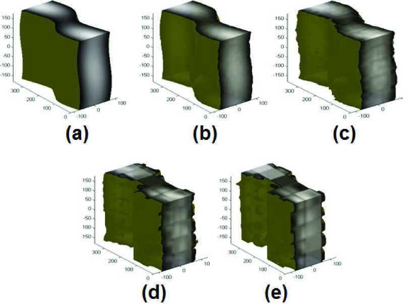
The torque function in configuration space of a three DOF climbing robot is depicted under different compression levels: (a) original data with memory volume of 64Kb; (b) 9Kb, MSE=2.86E-4; (c) 2Kb, MSE=0.002; (d) 0.6Kb, MSE=0.008; (e) 0.2Kb, MSE=0.0154
A well known quantification of image smoothness is Shannon's entropy, defined as Σ pi log pi 2, where pi denotes the probability for two i-distant voxels being identical (see [13]). Figure 4 exemplifies how a given configuration space calculated for varying resolutions becomes smooth as the resolution refines. So, refining calculations may increase the raw data volume on the one hand, while assisting the compression process on the other. High frequency coefficients in a building block translate to abrupt changes in the torque map. Obviously, this is not physical, so one may quantize the DCT coefficient block by storing only the AC coefficients “close enough” to the DC coefficient in the DCT block. The remaining coefficients, after the quantization, are set to zero. This also rescales the coefficients, ensuring an even smaller volume.

A four degree torque map entropy in different resolutions calculated from Δθ = 5 up to Δθ = 40.
We decode the required block by simply reversing the previous stages. In practice the block size (N) has a fixed size, which depends on the dimension of the configuration space, while the number of blocks depends on the configuration space resolution. Therefore, in order to accelerate the DCT transformation hardware parallel implementations were suggested [14–16].
3.1 The Quantization Matrix
An important step in the compression process is quantization. If the DCT coefficients were stored using lossless compression, only images with high periodicity would benefit from the compression algorithm. This is because certain frequencies would be significant, while the rest would have an amplitude of zero. Referring to 2D image processing language, the JPEG compression standard takes advantage of the human eye's relative insensitivity to high frequencies in order to compress images. By choosing a quantization matrix, e.g. a fixed set of 8 d elements, as divisors for the DCT coefficient dividends, we expect that the quotients of most of the high frequency coefficients will be of a negligible magnitude. Hence, via entropy coding, the image can be significantly compressed. Similarly, when compressing configuration spaces for motion planning, we are not preoccupied with high frequency changes, therefore we can use a quantization matrix whose coefficients are proportional to their rectilinear distance from the origin. The DC coefficient will be divided by 1, the neighbouring coefficients by 2 and so on. In fact we may expect high frequencies of negligible magnitudes, since the torque doesn't vary significantly with small perturbations of the robot's configuration.
4. Individual Compressions
There may be cases in which the map that needs to be compressed is not available in some forbidden configurations. For example, in our inchworm the torque map can be calculated for the entire configuration space including obstacle colliding configurations. This cannot be done in a configuration space lacking an analytic weight function (such is the case when data is collected from sensors). These configurations may take a large portion of the configuration space (see [4]). Again, in our inchworm inspired robot the forbidden region comprises 28% of the total space. Building blocks consisting of solely permitted (forbidden) configurations are compressed with great accuracy, however, if no special measures are taken, blocks that intersect the boundary of the free space and the forbidden region will be compressed with low accuracy due to the discontinuities at the boundaries. Thus, we should differentiate our treatment of the free space and the obstacle region using distinct compression techniques for each, considering their different nature.
Yet, simply applying the DCT technique outlined previously is problematic due to the discontinuities at the boundary of the obstacle. Obviously, this could be solved by defining a continuous (virtual) extension of the smooth data at the obstacle region while the obstacle region is compressed independently. There are several smoothing schemes that can be applied before compressing the configuration space. A quick yet naive approach is assigning all voxels of an obstacle region with the average value of the obstacle free space voxels bounding that area. Another method involves traversing through the forbidden region, assigning each forbidden node with the average of its neighbours' values. This technique has a high overhead since it requires sampling the same node a multiple number of times, until it has a sufficient amount of neighbours possessing a valid value. This method, however, has better smoothing capabilities than the previous one. It should be noted that applying a smoothing scheme results in a longer compression stage. This is not critical as our goal is to reduce the runtime at the decompression stage, which is unaffected by this enhancement.
4.1 Obstacle Region Compression
As noted above, binary information should be stored regarding each node character (either permitted or forbidden). There are several compression algorithms that can be used to compress the obstacle space. We now shall review some: (1) The chain code [17] is a lossless compression algorithm used for monochrome images can be adapted. This algorithm is highly effective for compressing the obstacle region since it is effective for images consisting of a large number of connected components; (2) Quad tree (generally 2n-tree) compression algorithms [18, 19] are slightly more suitable for the task of obstacle compression and may be generalized for multidimensional data. In order to improve the compression ratio one may allow obstacles to be slightly larger than their actual size. This one-way controlled error method allows one to trim a branch in the compression tree if only a few of its values are valid (i.e., almost all the nodes are obstacles). In our experience, this method significantly improves the obstacle region compression ratio and rarely discredits a valid solution; (3) Locating primitives [20] involves searching for specific shapes, such as spheres or capsules, which require the storage of several values such as two spherical centres and a radius. Since we expect the forbidden space to be grouped in clusters, this algorithm can be very efficient. It should be noted that while disregarding some of the free space is acceptable, disregarding some of the obstacle region is not allowed since the robot must not collide with any obstacle. Following this one could relax the problem, making it more efficient. A simpler version of this algorithm can be implemented by searching for multi-dimensional Cartesian cuboids. This way only the opposing vertices need to be stored. The disadvantage, of course, is the low efficiency of capturing cuboids, which is not aligned with the Cartesian axis (see [21]). Once the maximal cuboid has been found it must be removed from the space in order for others cubes not to intersect it. Otherwise, future cuboids that overlap previously found cuboids may be returned; (4) Probabilistic clustering, which randomly samples forbidden configurations. These can then be convexed in order to form a set of obstacle polytopes. Obviously, we need these polytopes to be as tight as possible within the obstacle manifold, leaving minimal obstacle space free. In order to do so one can apply a genetic algorithm (GA): First construct a population of such polytope spaces (which covers all obstacles in the configuration space) following the above procedure. Next, a fitness function grades each solution in the population and the GA optimizes the solution.
We exemplify this method on a 3-DOF robot. The result is depicted in Figure 5. The simplest, yet most efficient, way of coding the obstacle space is by using known geometric constraints within the workspace and translating those to the configuration space. Indeed, in our example these constraints are explicitly known, allowing us to apply the latter.

a. The real obstacle manifolds. b. A 500 randomly selected forbidden configurations where generated. c. These form an unsatisfying solution after the convex hull process (compare with Figure 5(a)). d. Using GA with population of 5 for 10 generation improves the solution
5. Experimentation
We shall now present some of the experiments done to prove the efficiency of our approach. We compare the compressed data with the original data by calculating the mean square error (MSE) and the data volume after quantization (see tables 1 and 2).
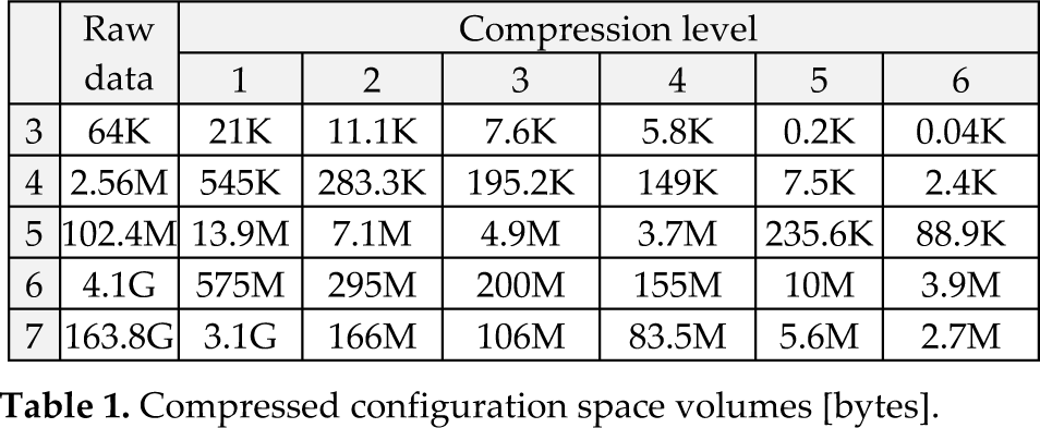
Compressed configuration space volumes [bytes].
MSE of the decompressed configuration space data normalized to the maximal (torque) value.

We used both schemes (4) and (5) from section 4.1 to compress forbidden space. Both presented essentially identical results. As for the smooth data, the algorithm divides the configuration space into (N/8)n building blocks, where n is the configuration space dimension and N is the number of voxels in each dimension (which in our case amounts to 5″ blocks). Each block is applied to a multidimensional DCT using MATLAB (see [22]). Elements in the quantization matrix A are valued:

(though different norms for the quantization matrices can be applied). In order for all DCT coefficients to vary within a given range we first subtract the mean value of that given block from each of its elements.
As the number of neighbouring voxels rises with the configuration space dimension, so does the autocorrelation. This in turn results in an improved compression ratio, as demonstrated in Figure 6.
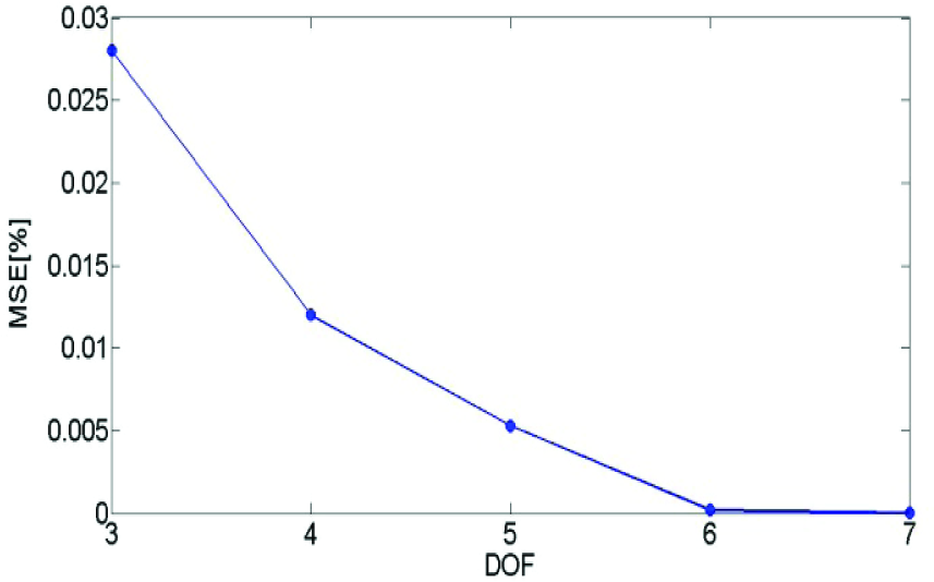
The MSE of the decompressed configuration space for varying DOF's climbing robot using a fixed threshold post quantization.
Tables 1 and 2 list a set of experiments for 3 to 7 degrees of freedom robots with thresholds varying from 0.01 to 20 (these where chosen to exemplify a large compression spectrum). Indeed, as figures in tables 1 and 2 demonstrate, the configuration space memory volume can be radically reduced by a factor of five orders of magnitude (× 105) when the dimension exceeds six and still maintain a reasonable accuracy.
To illustrate the usability of the decompressed data we used the naive Road Map algorithm in solving a motion planning problem for the 6 DOF case. The algorithm randomly and uniformly chooses a set of 50 anchoring points in the free space and calculates the weight (if it exists) between all pairs. This is done by checking the distance from all the neighbours of a current configuration in free space to the goal configuration and picking the closest neighbour, or setting the pair as not connected if the above is not found. For comparison, the same anchoring points are given for the original and restored data. Figure 7 compares motion planning using raw data configuration space and restored configuration space data as described above. Notice that the chosen roadmap vertices are all identical (for both experiments) but one. Since a lossy compression is performed (88kB remains of the 47MB raw data), the differences between the two data sets caused the last tree-edge to weigh more in terms of the torque map. This in turn, makes the Dijkstra algorithm pick an extra vertex (see Figure 7(1)). Calculating the power of local consumption differences in the experiment yields

6. Conclusions
Redundant mechanisms that lack an analytic weight function over their configuration space (or such with an obstacle space that is hard to mathematically formulate) often acquire their data via sensors (or simulation). For most robots, common weight functions such as energy or torques are smooth in the sense of Shannon's entropy and hence are compressible (see Section 3).
Experimentation indicates that configuration spaces' volumes may be compressed (using well known compression methods) in orders of magnitude, while maintaining an applicable accuracy (see Section 5). Binary data can be compressed and then integrated separately (Section 4). This approach is expected to be beneficial for embedded control systems where storage volumes are an expensive resource, while parallel computing may rapidly compress and de-compress data while the shortest path is computed. It should be noted that the compression process is time consuming (although only needed to be executed once). For example, a 6 DOF configuration space compression took hours to perform. Future work may address this issue by means of parallel computing. We may also make use of compression ratios varying with configurations (see Section 3) in order to further compress the data and speed up the compression process.