
Abstract
This paper aims to demonstrate a clear relationship between Lagrange equations and Newton-Euler equations regarding computational methods for robot dynamics, from which we derive a systematic method for using either symbolic or on-line numerical computations. Based on the decomposition approach and cross-product operation, a computing method for robot dynamics can be easily developed. The advantages of this computing framework are that: it can be used for both symbolic and on-line numeric computation purposes, and it can also be applied to biped systems, as well as some simple closed-chain robot systems.
Keywords
1. Introduction
When looking at robotics research, dynamic modelling is basically a form of artwork. The complexity of a dynamic model concerns the degrees of freedom (DOFs) of a machine or a robot and the dynamic model of a low DOFs robot can be easily developed, but dynamic models for a high DOFs robot are difficult to derive by hand. The drawbacks to creating the models by hand are: difficulty of maintenance, complexity of proofreading the dynamic model and inflexibility. The biped robot is the target of a complex dynamic system study [1] that also reveals a demand for a computer-aided systematic derivation tools for robotics.
Using an auto-deriving tool to obtain a dynamic model of a robot is very economical. Tošic [2] proposed the benefits of a symbolic simulation of an engineering system, while Cetinkunt [3] proposed a symbolic modelling of the dynamics of robotic manipulators on the numerical tool REDUCE. Since the coding of REDUCE is based on C and Fortran, modifying the system model by simply changing the symbol is rather difficult. Vibet demonstrated the symbolic tool FORM [4], which automatically generates the dynamic equations of the manipulator. The MACSYMA tool was then introduced to mechanical engineering education [5], providing the steps for determining a system dynamics model, but it does not support online simulations that integrate both system models and control rules.
Numerous contributions in both algorithms and their computational efficiency have been made in the field of robot dynamics [6–9]. The need for an online computing [6] method is motivated by simulation studies of the dynamics of a robotic system with large DOFs. While computation efficiency continues to be crucial for the simulation and control of increasingly complex mechanisms operating at higher speeds, other aspects of the dynamics problem are also vital. Algorithms should be formulated under a simple framework to enable ease of development, modification, extension and understanding.
This paper aims to demonstrate a clear relationship between Lagrange equations and Newton-Euler equations regarding the computational methods for robot dynamics, from which we derive a systematic method using either symbolic or on-line numerical computations. First, this study reviews the Lagrange formulation, as well as its symbolic generation method, which is suitable for studying a low-DOF robotic system. Second, based on the decomposition approach and cross-product operation, a computing framework can be easily developed to calculate the inertia matrix, the Coriolis and centrifugal matrix, and the gravity force vector of robot dynamics equations. The advantages of this computing method are that: it can be used for both symbolic and the on-line numeric computation purposes, and it also can be applied to a closed-chain robot system. We present several robotic system examples to demonstrate the versatility of the proposed method.
2. Decomposition method
Assume that a robot system has a generalized coordinate with n DOFs and let q = [q1 q2 ṫ qn]T. The equation of robot motion [9] can be written as

where the inertia matrix D is an n×n positive-definite symmetric matrix, C is an n×n Coriolis and centrifugal matrix, and G is an n×1 gravity force vector. The control input u = u1 u2 ṫ un] T is the vector of joint input forces or torques, and ui ≡ 0, if the i-th joint is not actuated. Significantly, C is not unique, and S = Ḋ − 2C is a skew-symmetric matrix caused by the null energy property.
2.1 Lagrange formulation approach
The total kinetic energy K of a robot consists of the rotational kinetic energy Kωi and the translational kinetic energy Kvi of each link. The total potential energy P consists of the potential energy Pi of each link; and therefore,

and

The kinetic energies Kωi and Kvi, and potential energy Pi of each link can be calculated as stated below. Let mi be the mass of link i and Ii be the inertia of link i expressed in the body-attached frame. Let Ri be the rotational matrix, ωi be the angular velocity and pci be the CoM (Centre of Mass) of link i. The angular velocity of link i can thus be expressed as

where

The potential energy of link i can be obtained by
where g is the acceleration of gravity and e3 = [0 0 1]T. The velocity of the CoM of link i can be computed by

where

From the Lagrange formulation, we have
and

The D, C and G matrices of the robot's equations of motion are then


and

2.2 Newton-Euler formulation approach
The decomposition of the robot's equations of motion can also be conducted using the Newton-Euler approach. The angular acceleration of link i is expressed as

where

and hence,

Since
which is the same as

Therefore, Dωi and Cωi can be obtained respectively using:
and

where
The acceleration of CoM of link i is
where
and hence,
Since

which is also the same as

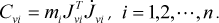
Therefore, the Dvi, Cvi and Gi matrices can be obtained by

and

2.3 Extended coordinate system
The Cartesian coordinates of the base point, [x0 y0 z0]
T
, are frequently added to form an extended set of generalized coordinates for the robot systems. Let qe = [x0 y0 z0 q1 ṫ qn]
T
be the extended coordinate system and next define the total mass

where
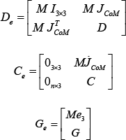
and

3. Procedures for computing the dynamic equations of a serial-link robot
Let mi be the mass of link i, Ii be the inertia of link i expressed in the body-attached frame and then q = [q1 q2 ṫ qn] T be the joint coordinate vector, where n is the number of joints. For simplicity, it is assumed that the relative motion of link i with respect to link (i-1) is either the rotational (revolute joint) or the translational (prismatic joint) motion with one of the basic axes in the local body frame from the set {± x-axis, ± y-axis, and ± z-axis} and is denoted by symbol ρi, where ρi ∈ {+Rx, −Rx, +Ry, −Ry, +Rz, −Rz, +Tx, −Tx, +Ty, −Ty, −Tz, −Tz}.
Define three basic rotational matrices: Rx(qi), Ry(qi), and Rz(qi), as shown below
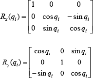
and

The procedures for computing the dynamic equation of a serial-link robot are thus as follows:
Step 1: Computing the rotational matrix of link i, Ri, i = 1, 2, ṫ, n
Let R0 = I3×3, and

Let ai and ti be the vectors of the corresponding rotational and translational axes of link i with respect to link (i-1), and then
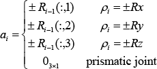
and
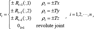
where R(:, k), k = 1,2,3 represents the k-th column of the matrix R.
Step 2: Computing the angular Jacobian matrix of link i, ωi = J ωiq̇, i = 1,2, ṫ, n
Let ω0 = 03×1, and

The angular Jacobian matrix of link i, Jωi, is
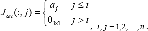
where Jωi (:, j) represents the j-th column of matrix Jωi and the total rotational kinetic energy K ω is obtained from
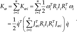
Matrix Dωi is formed by

Step 3: Differentiation of the angular Jacobian matrices The angular acceleration of link i is obtained as

where

Matrix Cωi is set up by

Step 4: Computing the linear Jacobian matrix of the CoM of link i, ṗci = Jviq̇, i = 1,2, ṫ, n
First, compute the joint position and CoM position of link i, pi and pci, i = 1, 2, ṫ, n. The linear Jacobian matrix of the CoM of link i,

The total translational kinetic energy Kv and the total potential energy P are obtained as

and

The matrices Dvi and Gi are set up as
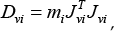
and

Step 5: Differentiation of the linear Jacobian matrices The linear acceleration of the CoM of link i is obtained as

where
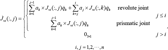
The matrix Cvi is equal to
Step 6: Putting it all together
The D, C, and G matrices of the robot's equations of motion are


and

4. Illustrated examples
4.1 Example 1: A 3 DOFs spherical robot
Figure 1 shows an example of a simple 3-DOF spherical robot system with both revolute and prismatic joints, and generalized coordinate q = [q1 q2 r] T , and is presented to verify the proposed computing method. The system parameters of the spherical robot are shown in Table 1 and the control input vector u = [u1 u2 u3]T. For a link with two joints, a virtual link with zero mass and/or zero inertia can be inserted for easy programming. The proposed method and the Lagrange method are shown to obtain the same equations of motion as follows
System parameters of the 3-DOF spherical robot system.


Example of a 3-DOF spherical robot system.

where

and

where ci = cos(qi), si = sin(qi), and i = 1,2.
4.2 Example 2: A 3-DOF robot system
Figure 2 presents an example of a 3-DOF robotic pendulum system with the generalized coordinate q = [q1 q2 q3]T. Table 2 lists the system parameters of this example and the control input vector u = [u1 u2 u3]T. The proposed method and the traditional Lagrange method are shown to obtain the same equations of motion,
System parameters of a 3-DOF robotic pendulum system.

Example of a 3-DOF robotic pendulum system.

4.3 Example 3: A 10-DOF biped robot
This example considers a 10-DOF fully actuated 3D biped with feet, as shown in Figure 3. The 3D biped robot consists of 7 links: a torso and two legs and two feet. Each leg has a knee and an equal length for the shin and thigh. The 10 actuators are installed as follows: two at the hip, one at the knee and two at the ankle. Table 3 lists the system parameters of this example.
System parameters of a biped robot.


Biped coordinate system when the left foot is the stance foot.
Let n = 10, the generalized coordinate q = [q1 q2 ṫ q10] T , and the control input vector u = [u1 ṫ u10]T. In the single-support phase, the biped's dynamic equation can be obtained as

where

and

Aside from the equations of motion, significant amounts of important data for the analysis of the biped's walking ability are also computed with minimal additional effort. For example, the biped ground reaction force F = [Fx Fy Fz] T and the zero moment point (ZMP) during the single-support phase [xzmp yzmp] T can be set up as:

and

where g is the gravity acceleration, pci = [xi, yi, zi] T is the centre of mass of the i-th link, and τi = [(τi) x , (τi) y , (τi) z ] T is the moment of the i-th link. For authentication, the 10-DOF biped robot online simulation work has been implemented on MATLAB. After symbolic calculation, we transfer the dynamic equations into C-Mex files to improve the efficiency of the biped robot walking simulation.
4.4 Example 4: A simple 2-DOF closed-chain robot
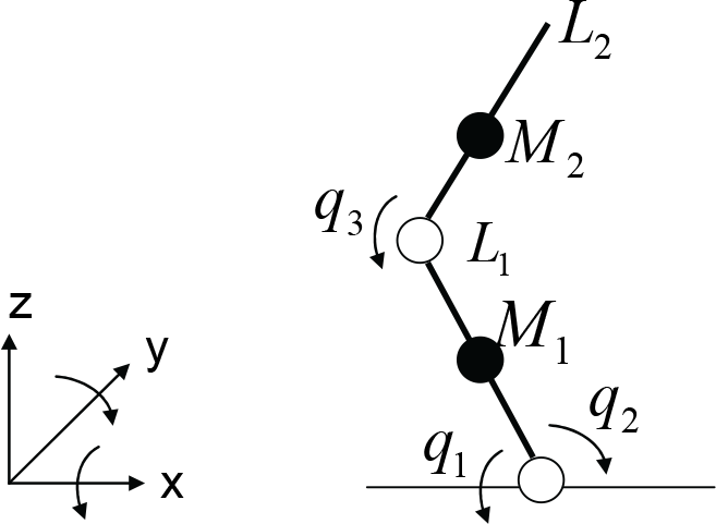
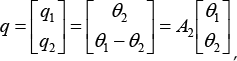
We can also apply the proposed method to calculate the equations of motion for simple closed-chain robotic systems. Figure 4 shows an example of a 2-DOF four-bar linkage robot system, where Link 1 and Link 4 are parallel links and their absolute angle θ1 is controlled by the input torque u1. Similarly, Link 2 and Link 3 are parallel links and their absolute angle θ2 is controlled by the input torque u2. The four-bar robot system can be treated as 2 serial-chain robot systems. The first serial-chain robot consists of Link 1 and Link 2 with generalized coordinates

An example of a 2-DOF four-bar linkage robot system.

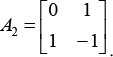
where

Similarly, the second serial-chain robot consists of Link 4 and Link 3 with generalized coordinates
where
For the first robot system, the system matrices D1, C1 and G1 can be calculated using the above method. For the second robot system, the matrices D2, C2 and G2 can be similarly obtained. The equations of motion for the four-bar linkage can thus be determined as:
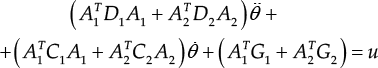
and hence
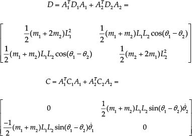
and

5. Conclusion
This paper has developed a decomposition and cross-product-based method to compute robot dynamics, offering several examples that demonstrate the versatility of the proposed method. The focus of this paper is first to establish a clear relationship between Lagrange equations and Newton-Euler equations, and second to develop an extremely intuitive and systematic method to compute the inertia matrix, the Coriolis and centrifugal matrix, and the gravity force vector of robot dynamics equations.
Footnotes
6. Acknowledgements
The work of C.L. Shih is supported by the Taiwan National Science Council (NSC) under Grant NSC 100-2221-E-011-020.