
Abstract
This paper discusses the stabilization and position tracking control of the linear motion of an underactuated spherical robot. Including the actuator dynamics, the complete dynamic model of the robot is deduced, which is a third order, two-variable nonlinear differential system that holds underactuation, strong coupling characteristics brought by the mechanism structure of the robot. Different from traditional treatments no linearization is applied, whereas a single-input multiple-output PID (SIMO_PID) controller is proposed with a neural network controller to compensate the actuator nonlinearity. A six-input single-output CMAC_GBF (Cerebellar Model Articulation Controller with General Basis Function) neural network is employed, while the Credit Assignment (CA) learning method is adopted to obtain faster convergence rate than the classical backpropagation (BP) learning method. The proposed controller can be generalizable to other single-input multiple-output system with good real-time capability. MATLAB simulations are used to validate the control effects.
Introduction
A spherical robot is a new type of mobile robot that has a ball-shaped outer shell to include all its mechanisms, control devices and energy sources inside it. This structural characteristic of a spherical robot helps protect the internal mechanisms and the control system from damage. At the same time, the appearance of a spherical robot brings a couple of challenging problems in modeling, stabilization and position tracking (path following). Two difficulties hinder the progress of the control of a spherical robot. One is the highly coupled dynamics between the shell and inner mechanism, and another is that although different spherical robots have different inner mechanism including rotor type, car type, slider type, etc (Joshi, Banavar and Hippalgaonka, 2010), most of them have the underactuation property, which means they can control more degrees of freedom (DOFs) than drive inputs. There are still no proven general useful control methodologies for spherical robots, although researchers attempted to develop such methodologies. Li and Canny (Li and Canny, 1990) proposed a three-step algorithm to solve the motion planning problems of a sphere, the position coordinates of the sphere can converge to the desired values in three steps. That method is complete in theory, but it can only be applied to spherical robots capable of turning a zero radius as the configurations are constrained. Mukherjee and Das et al. (Das and Mukherjee, 2004), (Das and Mukherjee, 2006) proposed a feedback stabilization algorithm for four dimensional reconfiguration of a sphere. By considering a spherical robot as a chained system Javadi et al. (Javadi and Mojabi, 2002) established its dynamic model with the Newton method and discussed its motion planning with experimental validations. As compared to other existing motion planners, this method requires no intensive numerical computation, whereas it is only applicable for their specific spherical robot. Bhattacharya and Agrawal (Bhattacharya and Agrawal, 2000) deduced the first-order mathematical model of a spherical robot from the non-slip constraint and angular momentum conservation and discussed the trajectory planning with minimum energy and minimum time. Halme and Suomela et al. (Halme, Schonberg and Wang, 1996) analyzed the rolling ahead motion of a spherical robot with dynamic equation, but they did not consider the steering motion. Bicchi, et al. (Antonio B. et. al., 1997), (Antonio and Alessia, 2002) established a simplified dynamic model for a spherical robot and discussed its motion planning on a plane with obstacles. Joshi and Banavar et al. (Joshi, Banavar and Hippalgaonka, 2009) proposed a path planning algorithm for a spherical mobile robot. Liu and Sun et al. (Liu, Sun and Jia, 2008) deduced a simplified dynamic model for the driving ahead motion of a spherical robot through input-state linearization and derived the angular velocity controller and angle controller respectively with full feedback linearized form.
Until now, for the control of spherical robots researchers mainly focused on the stabilization and motion planning of the “ball-plate” system, whereas the inner mechanism dynamics of a specific spherical robot was rarely considered and the underactuation characteristics of the spherical robot was not explored enough. In view of that case, the representive linear motion control of an underactuated spherical robot BHQ-1 developed in our lab is researched in this paper including the stabilization and position tracking issues. The remainder of this paper is organized as follows: In section 2, after a brief introduction of a spherical robot BHQ-1 the linear motion dynamic model with actuator dynamics of the robot is deduced. In section 3, the neural network control strategy is proposed. Four simulations are given in section 4. Section 5 concludes the paper.
Linear Motion Dynamics Model of BHQ-1
Preliminaries of BHQ-1
The mechanical structure of BHQ-1 is shown in Fig. 1. BHQ-1 consists of two motors, a hollow shaft, a counter-weight pendulum, a camera and a shell. The hollow shaft connected with the shell at two ends through ball bearings serves as a frame to install other devices. The output axle of motor 1 is fixed to the shell and the output axle of motor 2 is fixed to the pendulum by a link. The camera can be used to take photos of environments.
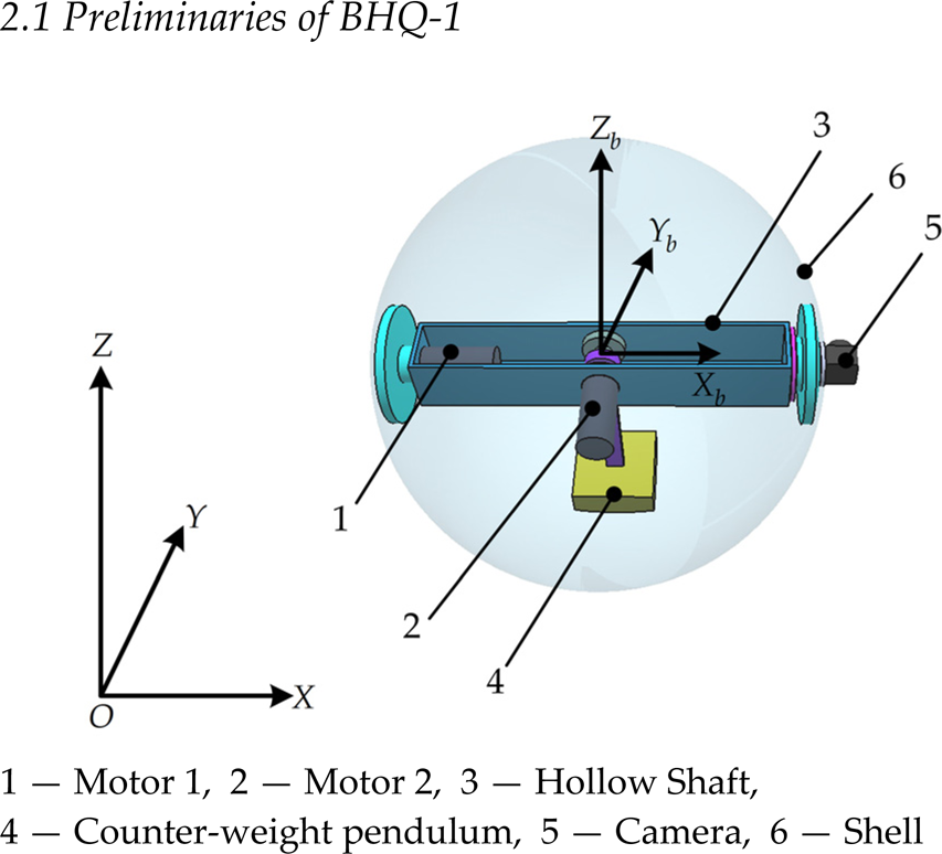
Structure of BHQ-1
The moving principle of BHQ-1 is as follows. When motor 1 rotates around axis X b and motor 2 keeps static, the rotation of the pendulum and the hollow shaft around axis X b changes the gravity center of the robot and produces a gravity torque that makes the robot move forward or backward. When both motor 1 and motor 2 rotate, the pendulum and the hollow axle will tilt and produce a gravity torque to make the robot veer. As a consequence, driven by two motors, the spherical robot can move and veer as anticipated. Therefore we can control the motion of the robot by controlling the two motors.
The spherical robot is modeled as a system with three components: the sphere shell, the inner drive unit (IDU) and the counter-weight pendulum. The friction of the internal mechanism and the sliding friction at the contact point between the outer shell and the floor are neglected. An important situation should be highlighted: If motor 1 provides more torque than what is necessary to hold the counter-weight pendulum at a horizontal position, the pendulum will deviate from the horizontal position or even rotate full circles within the sphere. When this occurs, the robot is uncontrollable (Tiu, Sun and Jia, 2008). For clarity, we assume that critical situation will not occur. The linear motion dynamics model of BHQ-1 is deduced under the following assumptions: 1) The spherical robot rolls following a straight-line without slipping; 2) No frictional forces exist in the internal mechanism; 3) The center of mass of the robot is consistent with the geometric center of the shell; 4) The counterweight pendulum is simplified as a particle hanging to the geometric center of the shell by a massless link; 5) The spherical shell has no thickness and its mass distributes evenly.
Fig. 2 depicts a simplified planar model of BHQ-1, where the coordinate ∑ o {X, Y} is fixed to the ground; V0 denotes the selected zero potential surface. The dynamic equations are derived by calculating the Tagrangian L = T − P of this system, where T and P refer to the kinetic energy and potential energy of the system, respectively.

Simplified planar model of BHQ-1
The kinetic energy of the system is computed as follows:
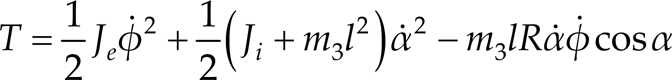
Where,

The potential energy is described as

Taking the swing angle of the pendulum, α, and the rolling angle of the robot, φ, as two generalized coordinates.

It is important to note that the input torque x of driving motor 1 works as an active inner force. By this notation, the Euler-Lagrange motion equations for the simplified system model are deduced as:

Under the pure rolling condition, we have
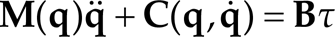
Where

The relationship between the rolling angle of the robot, φ, the motor-shaft position, q m , and the swing angle of the pendulum α is given by

For armature-controlled DC motors, the electrical model of driving motor 1 is characterized by
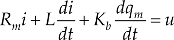
Where, i denotes the motor armature current.
Furthermore, the input torque produced by driving motor 1 is related to the armature current by
Where, K t > 0 is a constant. Substituting equation (8) into equation (7) yields

Where

Remark: The indicated inverse in equation (10) exists due to the physical nature of N and K t .
Substituting equation (5) and equation (6) into equation (9), the combined robot dynamic model yields

Where,

q(3) denotes the third partial time derivative of q.
Controller Design
Equation (5) presents an underactuated system with one input, τ, and two outputs, α and x. Respecting for the underactuated control of system (5), we employ a single-input two-output PID controller (Kishida Y. et. al., 1999) as shown in Fig. 3, which extends the PID controller for the single-input single-output case.

Scheme of the SIMO_PID controller
In Fig. 3, x d and α d represent the desired robot position and swing angle of the pendulum respectively. Using the SIMO_PID controller, the system with dynamic equation (5) can be controlled well. If considering the actuator dynamics, this control strategy exhibits poor performance for the required control input is changed to be the voltage instead of the torque whereas the voltage has strong coupling with the velocity due to the DC motor dynamics. In view of that case, a neural network compensation scheme (NNCS) as shown in Fig. 4 is proposed under the inspiration of reference (Jung, Cho and Hsia, 2007). Although Jung (Jung Cho and Hsia, 2007) put forward a decentralized neural network reference compensation technique (RCT) with good experimental results of the position tracking of a two-axis inverted pendulum system, that RCT was designed as based on the BP neural network that serves as a compensator for all the six components of two parallel PID controllers. The BP neural network (NN) has a complex 12 × 9 × 6 structure which results in large calculation cost and low real-time capability. Comparing with that RCT, the proposed NNCS has a simplified structure, which combines the SIMO_PID controller with a six-inputs one-output NN for compensating the uncertainties.

NN compensation control strategy for the linear motion control of BHQ-1
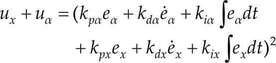
In Fig. 4, the control input u is composed of the pendulum angle control input uα, the robot position control input u x and the neural network compensation control input u n as

with the notation

Where, the pendulum angle GITOr eα, eα = α d − α, the robot position error e x , e x = x d − x.
When a neural network servers as a controller, the learning algorithm is critical for efficient online learning and control. Online learning and control is more preferred in a real control system design. For the linear motion control of BHQ-1, we employ a CMAC_GBF (Chiang and Tin, 1996) (Cerebellar Model Articulation Controller with General Basis Function) with the credit assignment (CA) learning technique (Su, Tao and Hung, 2003) as the NN, considering the advantages of CMAC_GBF such as speed, guaranteed learning convergence, capability of derivative, etc.
CMAC_GBF Structure
The CMAC_GBF neural network represents one kind of associative memory technique. In the addressing technique, each state variable (input) is quantized and the problem space is divided into discrete states. A vector of quantized input values specifies a discrete state and is used to generate addresses for retrieving information from memory for this state. The input vector,
Element y
s
of the output vector
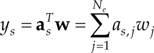
Where, N
e
is the number of elements in a complete block,
In CMAC_GBF, a general basis function b i (·) is used to replace the constant value stored in every hypercube. The value w i stored in a hypercube in a differentiable CMAC_GBF can be expressed as W i (x s ) = v i b i (x s ), and the output is rewritten as following:

A Gaussian function is adopted as the basis functions,

with the notation

Where m ij is the mean and σ ij is the variance, N v represents the number of variables in the target function. Consequently, the weight function is

The output from the CMAC with the Gaussian basis function can be mathematically expressed as

The error-feedback method is adopted for online learning of the CMAC_GBF. The control input u in equation (12) is chosen as the reference signal. Let the objective function be given by
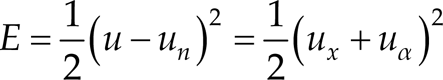
with the notation
At the convergence of (u − u n ) such as u n = u, all tracking errors are zero, that is to say, only CMAC_GBF provides the control input for the desired robot position and swing angle of the pendulum.
Differentiating equation (20) with respect to v i yields the gradient

The updated amount for v i can be set equal to

Where, f(i) is the trained times of ith hypercube, k denotes the addressed hypercubes for a state, μ v refers to the learning rate for v under the CA technique. Equation (23) suggests that the effects of error correcting depend on the inverse of learning times. The assumption is that the more times the memory has been trained, the more accurate the store value should be.
The means and variances of the Gaussian functions can also be adjusted to increase the approximation capability. The updating rules for these two parameters can be derived as:


where μσ, μ m are the learning rate for the variances and means under CA.
The simulation studies are performed in MATTAB, where the dynamic equation (5) and equation (11) as well as controllers described by Fig. 3 and Fig. 4 have been implemented. As discussed above, dynamics equation (11) includes the actuator dynamics but dynamics equation (5) does not. Those simulation studies are organized as following:
The simulation results are obtained by using the actual parameters of BHQ-1 prototype, which include:

The parameters of PID controllers are constant in all simulation studies, which are
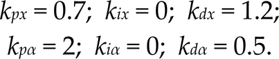
The parameters of CMAC_GBF are chosen as
The initial robot position and initial swing angle of pendulum of BHQ-1 are the same in the simulations: x(0) = 1, α(0) = 0. For the simulations of stabilization, the reference position and reference swing angle are: x d (t) = 0, α d (t) = 0; while x d (t) = 0.5t, α d (t) = 0 for the simulations of position tracking control, that is to say the robot runs at a constant speed 0.5m/s.
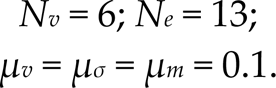
Fig. 5 shows the results of simulation study (a) and Fig. 6 presents the results of simulation study (b). In both Fig. 5 and Fig. 6, the dashed lines represent the reference motion and the solid lines refer to the simulated motion of BHQ-1.

Simulation study (a)
Simulation study (b)
From Fig. 5 it can be seen that SIMO_PID can realize the stabilization with a small overshoot occurring at about 7s. However, under the consideration of actuator dynamics (7), SIMO_PID shows poor control performance, it fails to stabilize the robot to a desired point as shown in Fig. 6. Without the actuator dynamics, the dynamic model of BHQ-1 is similar to the dynamic model of well-known cart-pendulum, crane, etc. Once considering the inner drive motor dynamics, the model becomes very complex, which turns to be a third order system. According to the mechanism structure of BHQ-1, the coupling relation between the two generalized freedoms (x and α) also becomes much more complex as depicted in equation (6) and equation (9). As a result that simulation study (b) also turns out that SIMO_PID takes no effect for that complex system.
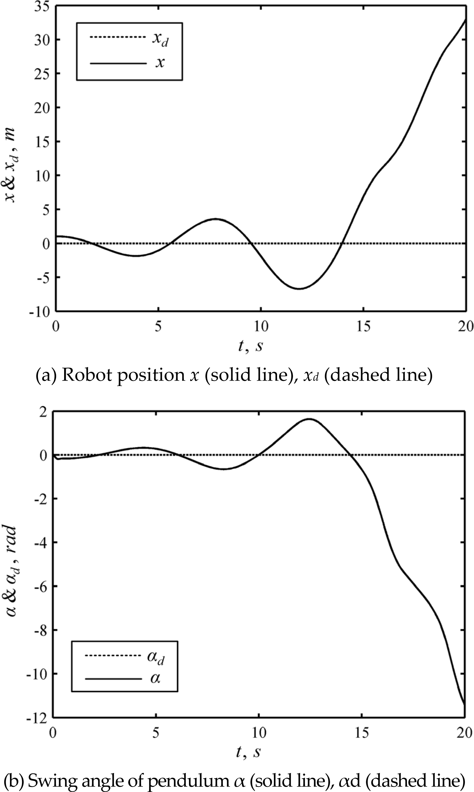
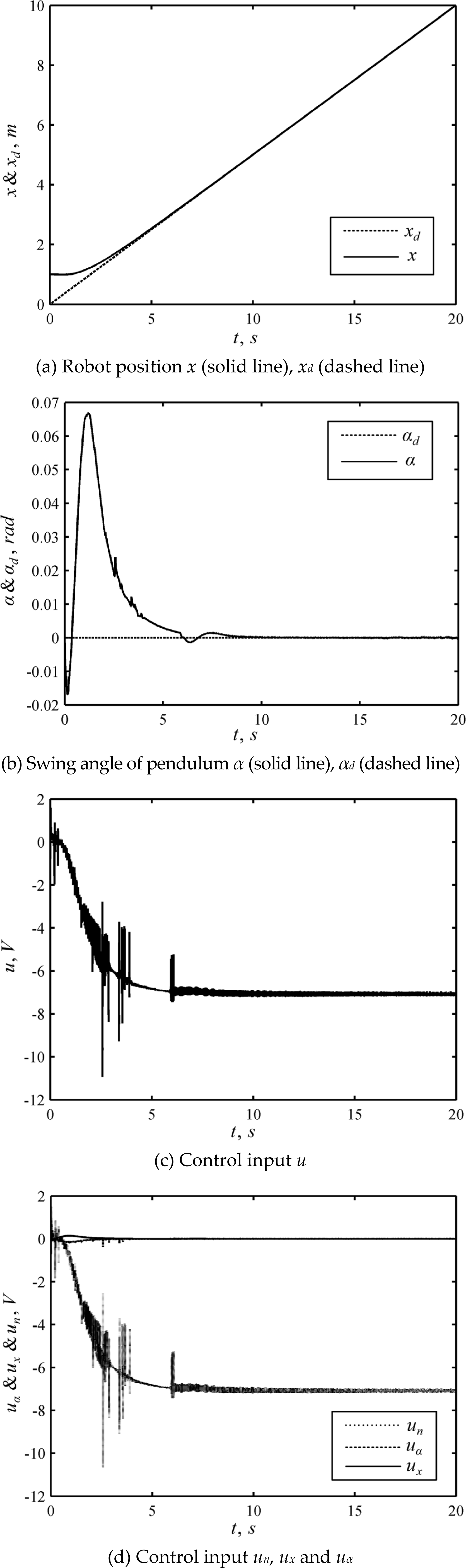
Under the control law (12), simulation studies are carried out for the stabilization and position tracking control of the dynamic model (11) and simulation results are shown in Fig. 7 and Fig. 8 respectively. Figures 7(a), 7(b) and 8(a), 8(b) show the reference motions and the simulated motions. Fig. 7(c) and Fig. 8(c) show the total control input. Figures 7(d) and 8(d) show more information such as the control input of PID controller for the robot position u x , control input of PID controller for the swing angle of pendulum uα and the control input of NN compensation u n .
Simulation study (c)
Simulation study (d)
In Figures 7(a), 7(b), 8(a) and 8(b), although a big initial error exists (e x (0) = 1, eα(0) = 0), the robot position x and the swing angle of pendulum α are successfully controlled to the desired motion with no overshoot. The response time is acceptable, which is less than 5s. With the NN compensation, the proposed controller (Fig. 4) exhibits its validity and good control performance. In Fig. 7(c) and Fig. 8(c), although the control input is not smooth, it is practically the motor armature input voltage which can vary instantaneously. From Fig. 7(d) and Fig. 8(d), it can be seen that after a learning process of short duration, the CMAC_GBF provides the main control input, which shows that the CMAC_GBF with CA learning method has a fast convergence rate and excellent learning precision.
In this paper, the stabilization and position tracking control of an underactuated spherical robot BHQ-1 moving straightly on a horizontal plane are researched. First the dynamic model is built without considering the actuator dynamics and a SIMO_PID controller is applied. Then, when the actuator dynamics is included, the SIMO_PID controller fails to control this complex system. In view of that case, a CMAC_GBF neural networks based compensation control scheme is proposed. Detailed design of the CMAC_GBF with CA learning method is presented. Furthermore, four simulation studies are performed to show the efficiency of this proposed control strategy with elaborate comparions. Future research on this method includes the real experiments on the BHQ-1 prototype and its generalization to the steering motion control of the spherical robot.
Footnotes
5.
This work is supported in part by National Natural Science Foundation of China under grant No. 50705003, National High Technology Research and Development Program of China under grant No. 2007AA04Z252 and “Blue Star Program” of Beijing University of Aeronautics and Astronautics.