Sage Journals: Discover world-class research

Abstract

This paper proposes a piecewise acceleration-optimal and smooth-jerk trajectory planning method of robot manipulator. The optimal objective function is given by the weighted sum of two terms having opposite effects: the maximal acceleration and the minimal jerk. Some computing techniques are proposed to determine the optimal solution. These techniques take both the time intervals between two interpolation points and the control points of B-spline function as optimal variables, redefine the kinematic constraints as the constraints of optimal variables, and reformulate the objective function in matrix form. The feasibility of the optimal method is illustrated by simulation and experimental results with pan mechanism for cooking robot.

Keywords

Optimal trajectory planning Cooking robot Pan mechanism

1. Introduction

Optimal trajectory planning is an active research field in robot manipulator. Most researches about the optimal trajectory planning aim at minimizing the execution time [1, 2], energy consumed [3, 4], and jerk [5, 6], under different conditions of several geometric, kinematic and dynamic constraints. Robot manipulators with high acceleration are urgently demanded in advanced manufacture fields, such as packaging and assembly of micro-electronic manufactures [7]. High acceleration means that robot manipulator completes pick-and-place operation in the shortest possible cycle time. On the other hand, high acceleration also will generate non-smooth jerk trajectories. High acceleration and non-smooth jerk is one pair of sharp contradiction. In addition, different segments of the path in some engineering applications will have different purposes, for example, shaping machine requires a smooth trajectory at the stage of slow cutting stroke, while a high velocity at the stage of quick return. In order to increase the efficiency of robot manipulator, the path should be divided into different segments based on the task of robot manipulator. Little research has been conducted to a piecewise acceleration-optimal and smooth jerk trajectory planning method.

The trajectory planning not only deals with the determination of the path, but also provides the velocity/acceleration profiles (or the time history of the robot's joints) [8]. Another less explored aspect of optimal trajectory planning is the determination of the velocity/acceleration profiles for the predefined path. Under such condition of the unchangeable path, the trajectory planner can only determine the velocity/acceleration values in the predefined path in order to improve the performance of robot manipulator. Such an aspect of optimal trajectory planning can be much more worthwhile in many robotic applications. For example, in machining applications, the velocity of the workpiece in the predefined path may have influences on the processing quality of the components.

Several researchers have investigated the optimal trajectory planning methods in recent years. Boryga etc. [9] put forward an optimal trajectory planning mode with higher-degree polynomials. The linear acceleration profiles of end-effectors were planned through the polynomials of degree 9, 7 and 5, and the minimal jerk was taken as an objective function. Gallina etc. [10] proposed a new technique for the optimal trajectory planning of a mobile robot. The trajectory was represented by a parametric curve consisting in sums of harmonics. Gasparetto etc. [11] proposed an optimal trajectory planning method, where the objective function containing a term proportional to the integral of the squared jerk and a second term proportional to the total execution time is considered. The proposed method did not consider the path in segments based on the task of robot manipulator. In order to generate a smooth jerk, Olabi etc. [12] presented a federate optimal trajectory planning method based on a parametric interpolation of the geometry in the operational space. Van Dijk etc. [13] developed a method for determining time-optimal trajectories for industrial manipulators along a predefined path, which accounts for actuator velocity, acceleration and jerk limits. Constantinescu etc. [14] discussed a method for determining smooth, time-optimal and path-constrained trajectory. The desired smoothness of the trajectory is imposed through limits on the actuator jerks. The time-optimal control objective is cast as an optimization problem by using cubic splines. Verscheure etc. [15] focused on time-optimal and time-energy optimal trajectory planning. Lou etc. [16] investigated and implemented three optimal trajectory planning methods based on dynamics limits. Saravanan etc. [17] applied a new general methodology to the optimal trajectory planning of industrial robot manipulator, which took the control points of the B-spline as the optimal variables and a multi-criterion cost function as the objective function. However, they ignored the importance of the time interval between two interpolation points. Vaz etc. [18] formulated robot trajectory planning as a semi-infinite programming problem and took the control points of B-spline as the optimal variables.

With a general literature survey, it come out that although more emphases have been laid on the multi-objective function in the whole path, the piecewise optimal method having multi-objective function is rarely applied in these researches. Another less explored but important objective function is the acceleration and jerk values in the predefined path. In addition, some of them only regard the control points of B-spline function as the optimal variables. Accordingly, the main goal of this paper is to propose a piecewise acceleration-optimal and smooth-jerk trajectory planning method, which takes both the time interval between two interpolation points and the control points of B-spline function as the optimal variables.

The remainder of the paper is organized in the following manner. In Section 2, the mathematical formulation of the optimal trajectory planning problem is developed. In Section 3, solution techniques for the formulated optimization problem are proposed to determine the optimal solution. Section 4 includes an illustrative example that demonstrates the utility of the optimal problem formulation and the feasible of applying these solution techniques for determining solutions. A few of cuisine experiments are carried out to verify the effectiveness of the optimal results. Some concluding remarks are included in the final section.

2. Optimal problem formulation

High acceleration and non-smooth is one pair of sharp contradiction in some engineering applications [7]. For purpose of solving the contradiction, trajectory will be divided into the “acceleration/deceleration” and “smooth” segments based on the task of robot manipulator. During the “acceleration/deceleration” segment, the maximum acceleration will be considered as the objective function. During the “smooth” segment, the expression of the smooth jerk will be added to the objective function. In the end, the objective function is given by the sum of two terms having opposite effects: the first term is proportional to the reciprocal of the integral of the squared acceleration during the “acceleration/deceleration” segment; the second term is proportional to the integral of the squared jerk during the “smooth” segment. Reducing the first term will lead to non-smooth jerk trajectory, while reducing the second term will lead to a faster trajectory. The trade-off between the two terms can be performed by suitably adjusting the weights of the two terms: a larger weight related to the jerk term will lead to smoother, while a larger weight related to the acceleration term will lead to faster trajectory.

On the basis of the above analysis, the piecewise acceleration-optimal and smooth trajectory planning problem can be formulated as follows:

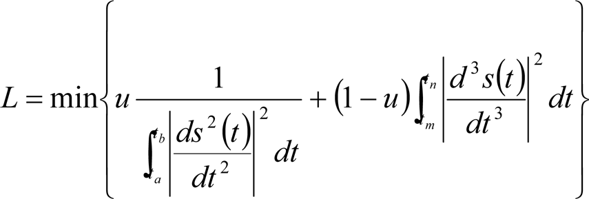
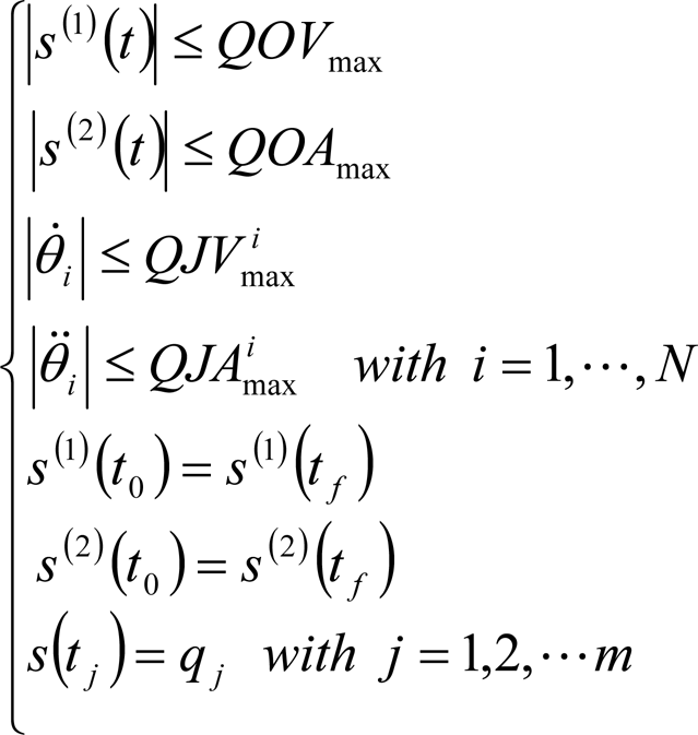
L = \min {u \frac{1}{\int_{t_{a}}^{t_{b}} {| \frac{d s^{2} (t)}{d t^{2}} |}^{2} d t} + (1 - u) \int_{t_{m}}^{t_{n}} {| \frac{d^{3} s (t)}{d t^{3}} |}^{2} d t}

(1)

Subject to the following constraints:

{\begin{cases} | s^{(1)} (t) | \leq Q O V_{\max} \\ | s^{(2)} (t) | \leq Q O A_{\max} \\ | {\dot{θ}}_{i} | \leq Q J V_{\max}^{i} \\ | {\ddot{θ}}_{i} | \leq Q J A_{\max}^{i} w i t h i = 1, \dots, N \\ s^{(1)} (t_{0}) = s^{(1)} (t_{f}) \\ s^{(2)} (t_{0}) = s^{(2)} (t_{f}) \\ s (t_{j}) = q_{j} w i t h j = 1, 2, \dots m \end{cases}

(2)

where U is the wei ght of the first term; s⁽¹⁾ (t), s⁽²⁾ (t) are the velocity and acceleration profiles of the trajectory; ${\dot{θ}}_{i}, {\ddot{θ}}_{i}$ are the angular velocity and acceleration of the ith joint; N is the number of the joints; QOV_max, QOA_max are the velocity and acceleration bound vectors; QJVⁱ_max, QJAⁱ_max are the velocity and acceleration bound values of the ith joint; t_a, t_b are the initial and final time values during the “acceleration/ deceleration” segment; t_m, t_n are the initial and final time values during the “smooth” segment; t₀, t_f are the initial and final time values of trajectory; m is the number of the interpolation points; and q_j are the interpolation points.

3. Solution techniques for optimal trajectory planning problem

3.1 Variables determination and constraints redefinition

The problem of computing a trajectory through multipoint can be solved by means of polynomial functions, orthogonal and trigonometric polynomials function, B-spline functions, and son on. Although B-spline function requires more information such as degree of the curve and a knot vector, and in general involve a more complex theory than other functions, it possess many advantages that offset this shortcoming. Firstly, some continuous derivatives and integral operators can be computed with relative ease from its spline coefficients. Further B-spline function can provide more control flexibility than other interpolation functions. In order to compute continuous derivatives up to four orders in this paper, the trajectories will be represented by B-spline function. For top-notch optimal performance, both the control points of B-spline function and the time interval between two interpolation points are chosen as the optimal variables. Thus, the optimal variables can be defined as follows:

X = {h_{0}, \dots, h_{n - 1}, p_{0}, \dots, p_{m}}

(3)

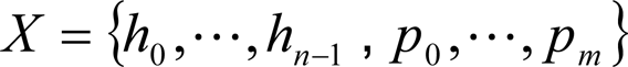
where h_i are time intervals between any adjacent two interpolation points; p_j are the control points of B-spline function; m and n are the numbers of the interpolation points and control points, respectively.

Definition 1. [19] The first and second derivatives of B-spline function s(t) can be obtained by differentiating the basis functions B^p_j(t).

{\begin{cases} s^{(1)} (t) = \sum_{j = 0}^{m - 1} \frac{p}{t_{j + p + 1} - t_{j + 1}} (p_{j + 1} - p_{j}) B_{j}^{p - 1} (t) \\ s^{(2)} (t) = \sum_{j = 0}^{m - 2} \frac{p - 1}{t_{j + p + 1} - t_{j + 2}} (\frac{p}{t_{j + p + 2} - t_{j + 2}} (p_{j + 2} - p_{j + 1}) - \frac{p}{t_{j + p + 1} - t_{j + 1}} (p_{j + 1} - p_{j})) B_{j}^{p - 2} (t) \end{cases}

(4)

where p_j is the control point; B^p−1_j (t) are the basis function of degree p − 1.

In order to implement easily the optimal formulation in computer, constraints inequalities (2) should be redefined as constraints of optimal variables of B-spline function. Given the velocity and acceleration bound vectors QOV_max and QOA_max, the first and second formulations in inequalities (2) can be expressed as follows:

{\begin{cases} {‖ s^{(1)} ‖}_{2} = \max_{j = 0, \dots, m - 1} | \frac{p}{t_{j + p + 1} - t_{j + 1}} (p_{j + 1} - p_{j}) | \leq Q O V_{\max} \\ {‖ s^{(2)} ‖}_{2} = \max_{j = 0, \dots, m - 2} | K_{j} p_{j} + K_{j + 1} p_{j + 1} + K_{j + 2} p_{j + 2} | \leq Q O A_{\max} \end{cases}

(5)

where

\begin{array}{l} K_{j} = \frac{p (p - 1)}{(t_{j + p + 1} - t_{j + 2}) (t_{j + p + 1} - t_{j + 1})}; \\ K_{j + 1} = \frac{- p (p - 1)}{(t_{j + p + 1} - t_{j + 2})} (\frac{1}{t_{j + p + 2} - t_{j + 2}} + \frac{1}{t_{j + p + 1} - t_{j + 1}}); \\ K_{j + 2} = \frac{p (p - 1)}{(t_{j + p + 1} - t_{j + 2}) (t_{j + p + 2} - t_{j + 2})} \end{array}

Given the velocity and acceleration bound vectors QJV_max and QJA_max of the joints, we also can formulate the following constraint inequalities about the third and forth formulations in inequalities (2).

{\begin{cases} \max_{j = 0, \dots, m} | p_{j} | \leq ‖ J^{- 1} ‖ Q J V_{\max} \\ \max_{j = 1, \dots, m - 1} (\frac{p}{t_{j + p + 1} - t_{j + 1}} (p_{j + 1} - p_{j})) \leq ‖ J^{- 1} ‖ Q J A_{\max} \end{cases}

where

{\begin{cases} \max_{j = 0, \dots, m} | p_{j} | \leq ‖ J^{- 1} ‖ Q J V_{\max} \\ \max_{j = 1, \dots, m - 1} (\frac{p}{t_{j + p + 1} - t_{j + 1}} (p_{j + 1} - p_{j})) \leq ‖ J^{- 1} ‖ Q J A_{\max} \end{cases}

(6)

where J is the Jacobian matrix of robot manipulator.

The fifth and sixth formulations in constraints inequalities (2) describe the periodic conditions on the velocity and acceleration. Given the interpolation points q_i(i = 1,···,m) and the control point's vector P = [p₀, p₁, ···, p_m−1, p_m]^T, the last three formulations in constraints inequalities (2) can be obtained as follows:

{\begin{cases} K_{0}^{(1)} p_{0} + K_{1}^{(1)} p_{1} + K_{m - 1}^{(1)} p_{m - 1} + K_{m}^{(1)} p_{m} = 0 \\ K_{0}^{(2)} p_{0} + K_{1}^{(2)} p_{1} + K_{2}^{(2)} p_{2} + K_{m - 2}^{(2)} p_{m - 2} + K_{m - 1}^{(2)} p_{m - 1} + K_{m}^{(2)} p_{m} = 0 \\ \sum_{j = 0}^{m} p_{j} B_{j}^{p} (t_{i}) = q_{i} w i t h i = 1, \dots, m \end{cases}

(7)

Since any time intervals between a pair of consecutive via-points can not be run at infinite acceleration and jerk, another type of constraint about any time interval h_i can be expressed as follows:

{\begin{cases} h_{i} > \max_{i = 0, \dots, n - 1} {\frac{| s^{(2)} (t_{i + 1}) - s^{(2)} (t_{i}) |}{Q O A_{\max}}} \\ h_{i} > \max_{i = 0, \dots, n - 2} {\frac{| s^{(3)} (t_{i + 1}) - s^{(3)} (t_{i}) |}{Q O J_{\max}}} \end{cases}

(8)

3.2 Reformulation of optimal objective function

For the convenience of the programming, the objective function in Eq. (1) defined in terms of B-spline can be formulated as follows:

L = \min {\frac{1}{t r (P^{T} C^{T} A C P)} + \frac{1 - u}{6 u} t r (P^{T} D^{T} B D P)}

(9)

being

\begin{array}{l} P = {[p_{0}, p_{1}, \dots, p_{m - 1}]}^{T} \\ A = d i a g {\int_{u_{0}}^{u_{n}} {| B_{j}^{2} (t) |}^{2} d u}, j = 0, 1, \dots, m - 1 \\ B = [\begin{matrix} 2 t_{2, 0} & t_{2, 1} & 0 & \dots & 0 \\ t_{2, 1} & 4 t_{3, 1} & t_{3, 2} & 0 & ⋮ \\ 0 & t_{3, 2} & 4 t_{4, 2} \\ ⋮ & 0 & t_{4, 3} & ⋱ & t_{m - 2, m - 3} & 0 \\ t_{m - 2, m - 3} & 4 t_{m - 1, m - 3} & t_{m - 1, m - 2} \\ 0 & \dots & 0 & t_{m - 1, m - 2} & 2 t_{m, m - 2} \end{matrix}] \\ C = [\begin{matrix} \frac{- p}{t_{p + 1, 1}} & \frac{p}{t_{p + 1, 1}} & 0 & \dots & 0 \\ 0 & \frac{- p}{t_{p + 2, 2}} & \frac{p}{t_{p + 2, 2}} & 0 & ⋮ \\ ⋮ & ⋱ \\ 0 \\ 0 & 0 & \frac{- p}{t_{p + m, m}} & \frac{p}{t_{p + m, m}} \end{matrix}] \\ D = [\begin{matrix} c_{0, 1} & c_{0, 2} & c_{0, 3} & 0 & \dots & 0 \\ 0 & c_{1, 1} & {ci}_{1, 2} & c_{1, 3} & 0 & ⋮ \\ ⋮ & ⋱ & 0 \\ 0 & \dots & 0 & c_{m - 2, 1} & c_{m - 2, 2} & c_{m - 2, 3} \end{matrix}] \end{array}

where

\begin{array}{l} c_{k, 1} = \frac{6}{t_{k + 4, k + 2} t_{k + 4, k + 1}}, \\ c_{k, 2} = - \frac{6}{t_{k + 4, k + 2}} (\frac{1}{t_{k + 4, k + 1}} + \frac{1}{t_{k + 5, k + 2}}), \\ c_{k, 3} = \frac{6}{t_{k + 4, k + 2} t_{k + 5, k + 2}}, t_{i, j} = t_{i} - t_{j}, \end{array}

and tr(P^TC^TACP);tr(P^TD^TBDP) are the trace of the matrix P^TC^T ACP and P^TD^T BDP, respectively.

3.3 Optimization methods

The optimal trajectory planning problem of a robot manipulator is a constrained nonlinear optimization problem. Some constraint equations have no explicitly analytical expressions with respect to the optimal variables. Furthermore, there may many local minima in the feasible search region. Some conventional optimization algorithms, e.g., the sequential quadratic programming (SQP) method, are known to converge to local minima. Compared with SQP, genetic algorithms (GA) can avoid the problems associated with local optima [20]. However, it should be known that the ability of local searching in GA is weak so that it would lead to convergence slow. It would be a good choice to design a hybrid GA by combining standard GA with other robust and fast algorithms. For strong ability of complex function approximation and remarkable speed in simulation, ANN will be chosen to be combined with standard GA to generate a hybrid GA-ANN algorithm, where ANN is utilized to represent expressions of the solutions, and the objective function is solved using GA. The combination of ANN and GA has been widely used in the field of materials science [21], chemical engineering [22, 23], robot manipulators [24], and heat transfer [25, 26]. In this section, three conventional and evolutionary optimization methods are utilized to solve the minimization problem formulated in Eq. (9), which is subjected some kinematic constraints in Eqs. (5), (6), (7) and (8).

3.3.1 Conventional optimal technique

The conventional iterative optimal techniques, such as sequential quadratic programming (SQP) have been widely applied to solve nonlinearly constrained optimization problems. As a form of the gradient-based optimal technique, SQP performs well in local search problems. But it can not assure that the calculated solution values are the global optimal value because of its relatively weak global search ability. Moreover, the optimal performance of SQP greatly depends on the choice of the initialization values. Improper initial values will lead to local optima or even infeasible solutions. The fmincon function in MATLAB'S OPTIMIZATION TOOLBOX, which uses the SQP method to perform nonlinear constrained optimization and support linear and nonlinear constraints, will be utilized to generate the optimal value of the optimal trajectory planning problem in this paper.

3.3.2 Genetic algorithm (GA)

Genetic algorithms, as a powerful and broadly applicable search method, follow the Darwinian evolutionary principle of “survival-of-the- fittest,” where strong traits are retained in the population and weak traits are eliminated. Thus, genetic algorithms can avoid the problems associated with local optima. There are three operations in genetic algorithms, such as selection, crossover and mutation. The parameters of genetic algorithms utilized in this paper are shown in Tab.1.

Table 1.
Parameters of genetic algorithm utilized in this paper

Genetic parameters Values

Population size 20

Uniform crossover (%) 80

Jump mutation rate (%) 1

Creep mutation (%) 2

Generation 500

Genetic parameters	Values
Population size	20
Uniform crossover (%)	80
Jump mutation rate (%)	1
Creep mutation (%)	2
Generation	500

3.3.3 Optimal method for hybrid GA-ANN algorithm

ANN model in the hybrid GA-ANN algorithm is designed and implemented using software developed in MATLAB 6.5 package. The back-propagation algorithm is used to minimize the instantaneous error in a particular training pattern. Additionally, the input parameters of the model are the optimal variables in this paper, and the output of the ANN is the optimal objective function. The ideal ANN model is considered to be obtained with single hidden layer and 15 neurons in it. The tansig and logsig function are employed as the activation functions between input-hidden layer and hidden-output layer, respectively.

4. An illustrative example

One example is provided to demonstrate the effectiveness of the piecewise acceleration-optimal and smooth trajectory planning method. Chinese culinary arts have a long history and are famous all over the world. Chinese dishes appeal to the senses through their color, aroma, taste, and appearance. However, its cooking process is extraordinarily complicated [27, 28]. For purpose of replacing the chef's cooking process motions by using the intelligent cooking equipment, we proposed a cooking robot including a pan mechanism, as shown in Fig. 1 [29, 30]. It consists of a moving platform and a 2-DOF pan mechanism. The 2-DOF pan mechanism, whose kinematics model is shown in Fig. 1(b), is fixed to the moving platform. The moving platform can move using a group of ball screws and a pair of linear guides. The 2-DOF pan mechanism is composed of nine bars (1) ∼ (8) and (9). The motion of the pan can be obtained through the two input angles θ₁ and θ₂, respectively. A fixed global reference frame G: OXY is located at the point A₂.

The most significant featured motion of the cooking process in Chinese cuisine is the motion of turning over the cuisine being cooked [30]. It can cause cuisines to continuously change position relative to pan, such as “ascent-descent”. Nevertheless, these position changes need to be accomplished through the variable acceleration motion of pan mechanism, which will be determined and optimized by the optimal trajectory planning method. Furthermore, the reduction of vibration, stemmed from the variable acceleration motion, will also be considered in the optimal trajectory planning method. Hence, it is of utmost importance to determine the acceleration and generate a smooth trajectory through the optimal trajectory planning method.

Figure 1.

Cooking robot and pan mechanism: (a) cooking robot; (b) kinematics model of pan mechanism

Table 2.

Values of the interpolation points and kinematics constraints

Interpolation points
	1	2	3	4	5	6
Values (mm/s)	241.46	687.2	146.24	394.16	256.63	241.46
Kinematics constraints
Velocity (mm/s)	Acceleration (mm/s²)	Jerk (mm/s³)
800	8400	200000

4.1 Prototype and parameters

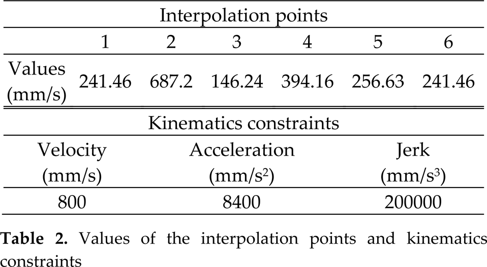
To facilitate the analysis, the dimensions of pan mechanism are given as follows: A₁B₁=0.11m, A₂B₂=0.019m, A₃B₃=0.08m, B₁C₁=0.14m, B₂C₂=0.096m, B₃C₃=0.23m, C₂B₁=0.08m, C₃C₁=0.07m. As shown in Fig. 2(a), its prototype was developed, and its path is shown in Fig. 2(b). The “ascent” segment is defined as the curve from A to B, while the “descent” segment is the curve from B to A. The values of the interpolation points and kinematic constraints are listed in Table 2.

Figure 2.

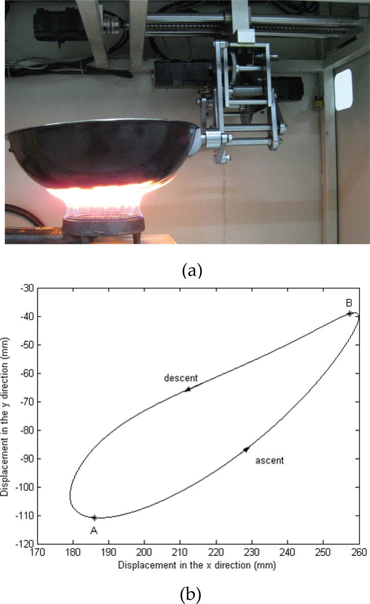
Prototype and path: (a) prototype of pan mechanism; (b) predefined path of pan mechanism

4.2 Numerical optimal results

The optimal result histories of the fmincon function, GA method and hybrid GA-ANN algorithm are shown in Fig. 3. The chief findings from Fig. 3 are as follows: (1) there are the same convergence pattern in both GA method and hybrid GA-ANN algorithm, i.e., both are in lower region. And the convergence velocity of hybrid GA-ANN is higher than other two methods. (2) In terms of objective function value, both GA method and hybrid GA-ANN algorithm provide the lowest optimal values in comparison with the fmincon function. Due to an unsuitable initial value, the fmincon function may converge to local minima. (3) Considerable reduction in computational time is achieved for the hybrid GA-ANN algorithm in comparison with other two methods. From the above analysis results, a conclusion can be drawn that hybrid GA-ANN algorithm is a superior method in terms of computational effort and solution accuracy.

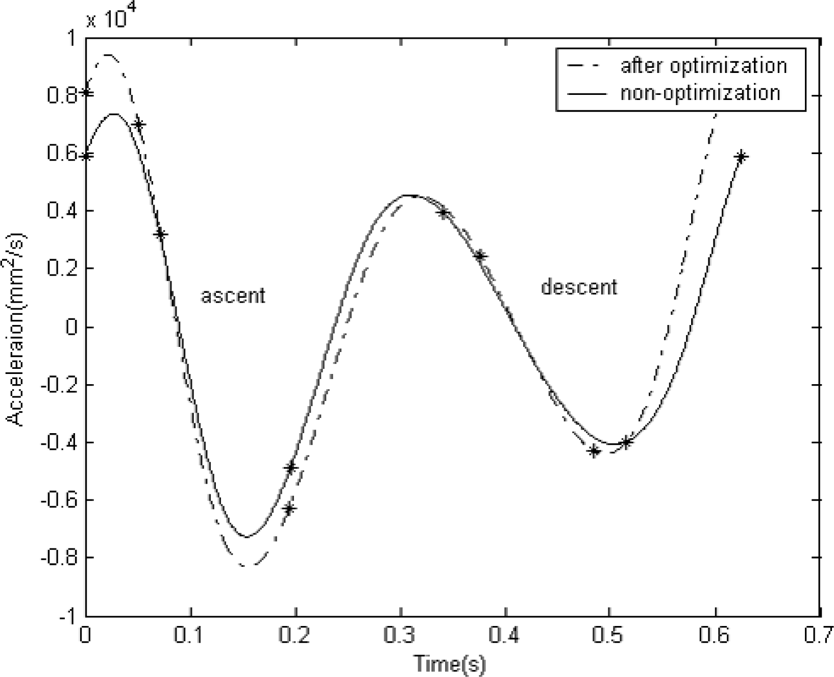
Then, the optimal results of acceleration using the hybrid GA-ANN algorithm are shown in Fig. 4. The labels “*” represent the interpolation points. During the “ascent” segment, the acceleration after optimization is higher than the initial acceleration, which is helpful to turn over the cuisine being cooked. During the “descent” segment, the total time is shortened through optimization, which will prevent the cuisine being cooked from adhering to the pan. We can draw a conclusion from Fig. 4 that during the “ascent” segment, the acceleration after optimization is more favorable for the motion of turning over the cuisine being cooked, and during the “descent” segment, the less time after optimization will prevent the cuisine being cooked from adhering to the pan.

Jerk values with the optimal objective function including jerk term and excluding jerk term are shown in Fig. 5. We can intuitively observe from Fig. 5 that the jerk values with the optimal objective function including jerk term are less and smoother than those with the optimal objective function excluding jerk term. Smoother jerk values will reduce the vibration of the cooking robot.

Figure 3.

Optimal result histories using three optimization methods

Figure 4.

Optimal results of acceleration

Figure 5.

Jerk values with the optimal objective function including jerk term and excluding jerk term

In the end, we can draw a conclusion that during the “ascent” segment, the acceleration after optimization is more favorable for the motion of turning over the cuisine being cooked, and during the “descent” segment, the less time after optimization will prevent the cuisine being cooked from adhering to the pan.

4.3 Experimental results

In order to testify the effectiveness of the optimal results, a few cuisine experiments, as shown in Fig. 6 have been conducted with fried green beans. Cuisines in Fig. 6(b) are turned over higher than those in Fig. 6(a). Thus, the optimal results will improve the quality of the cooking.

Figure 6.

Dish-cooking experiments with fried green beans: (a) the non-optimal velocity; (b) the optimal velocity

As shown in Fig. 7, a test system for measuring the acceleration of pan mechanism is composed of acceleration sensor, charge amplifier, signal adjust circuit and data acquisition card, and so on. From Fig. 7(a), it is observed that the acceleration sensor is installed at the center of pan. Fig. 8 shows the acceleration signal of pan mechanism obtained by the test system. Although there existing some measuring errors caused by installation clearance, the following common characteristics between the theoretical values in Fig. 4 and the experimental values in Fig. 8 can be obtained: (1) there existing a maximal acceleration during the “ascent” segment, which results in the motion of turning over the cuisine being cooked. (2) The acceleration values during the “ascent” segment after optimization are greater than the initial acceleration.

Figure 7.

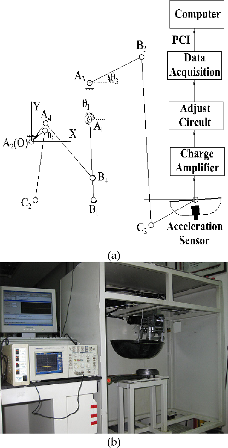
Test system of pan mechanism: (a) schematic diagram of test system; (b) experimental system

Figure 8.

Acceleration signal obtained by the test system

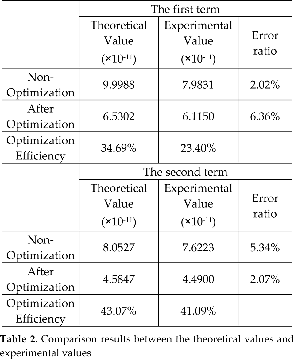
The comparison results between the theoretical values and experimental values are shown in Tab.3. Both the theoretical values and experimental values after optimization are superior to those initial values. And, the optimization efficiency is improved by approximately 40%. Hence, we can draw a conclusion from the comparison results that these optimization results will provide a powerful support to the motion of turning over the cuisine being cooked, however, the error rates between the theoretical values and experimental values are still very great.

Table 2.

Comparison results between the theoretical values and experimental values

	The first term
	Theoretical Value (x10⁻¹¹)	Experimental Value (x10⁻¹¹)	Error ratio
Non-Optimization	9.9988	7.9831	2.02%
After Optimization	6.5302	6.1150	6.36%
Optimization Efficiency	34.69%	23.40%
	The second term
	Theoretical Value (x10⁻¹¹)	Experimental Value (x10⁻¹¹)	Error ratio
Non-Optimization	8.0527	7.6223	5.34%
After Optimization	4.5847	4.4900	2.07%
Optimization Efficiency	43.07%	41.09%

5. Conclusion

A piecewise acceleration-optimal and smooth-jerk trajectory planning problem for robot manipulator along a predefined path was defined as an optimal B-spline function that takes both the time interval and the control points as the optimal variables, and results in minimal jerk value and maximal acceleration value. Some computing techniques were proposed to determine the optimal solution. These techniques transformed the kinematics constraints into the constraints of the optimal variables, and reformulated the objective function as matrix form.

A few of cuisine experiments were carried out to verify the effectiveness and feasibility of the optimal results. Future works will include utilizing the techniques developed here as the basis for solving other application, so as to validate the generality of the algorithm. Substantial further work will be paid to the control scheme for the robotic manipulator and further adjust the optimal parameters in a certain field.

Footnotes

6.

The work was supported by the National Natural Science Foundation of China (Grant No. 60875060,51175105).

References

Constantinescu

Croft

E.A.

, “Smooth and time-optimal trajectory planning for industrial manipulators along specified paths,” Journal of Robotic Systems, vol. 17(5), pp.233–249, 2000.

Pateloup

Duc

and Ray

, “Corner Optimization for pocket machining,” International Journal of Machine Tools and Manufacture, vol. 44(12–13), pp. 1343–1353, 2004.

Saramago

S.F.P.

Steffen

, “Optimal trajectory planning of robot manipulators in the presence of moving obstacles,” Mechanism and Machine Theory, vol.35, pp.1079–1094,2000.

Kim

H.J.

Kim

B.K.

, “Minimum-energy trajectory planning on a tangent for battery-powered three-wheeled omni-directional mobile robots,” in: International Conference on Control Automation and Systems (ICCAS), Gyeonggi-do, 2010, pp.1701–1706.

Huang

P.F.

Y.s.

, and Liang

, “Global Minimum-Jerk Trajectory Planning of Space Manipulator,” International Journal of Control, Automation, and Systems, vol. 4 (4), pp. 405–413, 2006.

Gasparetto

Zanotto

, “A technique for time-jerk optimal planning of robot trajectories,” Robotics and Computer-Integrated Manufacturing, vol. 24 (3), pp.415–426, 2008.

Nabat

Krut

Company

Poignet

and Pierrot

, “On the Design of a Fast Parallel Robot Based on Its Dynamic Model,” Experimental Robotics, vol. 39, pp. 409–419, 2008.

Raza

U.R.

Stéphane

Damien

Philippe

, “Multiobjective Path Placement Optimization of Parallel Kinematics Machines Based on Energy Consumption, Shaking Forces and Maximum Actuators Torques: Application to the Orthoglide,” Mechanism and Machine Theory, vol.45(8), pp. 1125–1141, 2010.

Boryga

Graboś

, “Planning of manipulator motion trajectory with higher-degree polynomials,” Mechanism and machine theory, vol. 44, pp. 1400–1419, 2009.

10.

Gallina

and Gasparetto

, “A technique to analytically formulate and to solve the 2-Dimensional constrained trajectory planning problem for a mobile robot,” Journal of Intelligent and Robotic System, vol. 27(3), pp. 237–262, 2000.

11.

Gasparetto

and Zanotto

, “A new method for smooth trajectory planning of robot manipulators,” Mechanism and machine theory, vol. 42, pp. 455–471, 2007.

12.

Olabi

Béarée

Gibaru

and Damak

, “Feedrate planning for machining with industrial six-axis robots,” Control Engineering Practice, vol. 18, pp. 471–482, 2010.

13.

van Dijk

N.J.M.

van de Wouw

Nijmeijer

, and Pancras

W.C.M.

, “Path-constrained motion planning for robotics based on kinematics constraints,” in: Proceedings of the ASME International Design Engineering Technical Conferences & Computers and Information in Engineering Conference, Las Vegas, 2007, pp. 1071–1080.

14.

Constantinescu

and Croft

E.A.

, “Smooth and time-optimal trajectory planning for industrial manipulators along specified paths,” Journal of robotic systems, vol. 17(5), pp. 233–249, 2006.

15.

Verscheure

Demeulenaere

Swevers

Schutter

Diehl

, “Time-Energy Optimal Path Tracking for Bobots: a Numerically Efficient Optimization Approach,” in: Proceeding of the 10th International Workshop on Advanced Motion Control, Trento, 2008, pp.727–732.

16.

Lou

Y.J.

Feng

and Wang

M.Y.

, “Trajectory planning and control of parallel manipulators,” in: IEEE International Conference on Control and Automation, Christchurch, pp. 1013–1018, 2009.

17.

Saravanan

Ramabalan

and Balamurugan

, “Evolutionary optimal trajectory planning for industrial robot with payload constraints,” International Journal Advanced Manufacturing Technology, vol. 38, pp. 1213–1226, 2008.

18.

Vaz

A.F.

Fernandes

E.M.G.P.

Gomes

M.S.F.

, “Robot trajectory planning with semi-infinite programming,” European Journal of Operational Research, vol. 153(3), pp. 607–617, 2004.

19.

Simon

, “Data smoothing and interpolation using eighth order algebraic splines,” IEEE Transactions on Signal Processing, vol. 52(4), pp. 1136–1144, 2004.

20.

Holland

, Adaptation in natural and artificial systems. Ann Arbor, MI: The University of Michigan Press, 1975.

21.

Sun

Zeng

W.D.

Liang

X.B.

Zhang

J.W.

, “A hybrid approach for processing parameters optimization of Ti-22Al-25Nb alloy during hot deformation using artificial neural network and genetic algorithm,” Intermetallics, vol. 19, pp. 1014–1019, 2011.

22.

Huang

Zhan

X.L.

Chen

F.Q.

D.W.

, “Catalyst design for methane oxidative coupling by using arti&cial neural network andhybridgenetic algorithm,” Chemical Engineering Science, vol. 58, pp. 81–87, 2003.

23.

Ahmad

A.L.

Azid

I.A.

Yusof

A.R.

Seetharamu

K.N.

, “Emission control in palm oil mills using artificial neural network and genetic algorithm,” Computers and Chemical Engineering, vol. 28, pp. 2709–2715, 2004.

24.

Gao

Zhang

Y.J.

, “Design optimization of a spatial six degree-of-freedom parallel manipulator based on artificial intelligence approaches,” Robotics and Computer-Integrated Manufacturing, vol. 26, pp. 180–189, 2010.

25.

Peng

Ling

, “Optimal design approach for the plate-fin heat exchangers using neural networks cooperated with genetic algorithms,” Applied Thermal Engineering, vol. 28, pp.642–650,2008.

26.

Kadiyala

P. K.

Chattopadhyay

, “Optimal location of three heat sources on the wall of a square cavity using genetic algorithms integrated with artificial neural networks,” International Communications in Heat and Mass Transfer, vol. 38, pp. 620–624, 2011.

27.

Tang

J.H.

Zhao

X.Y.

Liu

X.Y.

, “On the Current Situation and Prospect of the Study of AIC,” Culinary Science Journal of Yangzhou University (in Chinese), vol. 2, pp. 24–26, 2007.

28.

Hou

, “The trends of industrialized development for Chinese cuisine and its principle,” Culinary Science Journal of Yang Zhou University(in Chinese), vol. 20, pp. 7–10, 2003.

29.

Chen

Deng

and Xu

, “Conceptual analysis and design of the 2T1R mechanism for a cooking robot,” Robotcs and Autonomous Systems, vol. 59, pp. 74–83, 2011.

30.

Chen

Deng

Z.Q.

, “Dynamic Modeling and Performance Analysis of a 3-DOF Pan Mechanism for a Cooking Robot,” Mechanics Based Design of Structures and Machines, vol. 38(2), pp. 243–260, 2010.

A Piecewise Acceleration-Optimal and Smooth-Jerk Trajectory Planning Method for Robot Manipulator along a Predefined Path

Abstract

Keywords

1. Introduction

2. Optimal problem formulation

3.1 Variables determination and constraints redefinition

3.3.1 Conventional optimal technique

3.3.2 Genetic algorithm (GA)

Table 1. Parameters of genetic algorithm utilized in this paper Genetic parameters Values Population size 20 Uniform crossover (%) 80 Jump mutation rate (%) 1 Creep mutation (%) 2 Generation 500

4. An illustrative example

Footnotes

6.

References

Table 1.
Parameters of genetic algorithm utilized in this paper

Genetic parameters Values

Population size 20

Uniform crossover (%) 80

Jump mutation rate (%) 1

Creep mutation (%) 2

Generation 500