Sage Journals: Discover world-class research

Abstract

This paper presents an alternative approach to implementing a stereo camera configuration for SLAM. The approach suggested implements a simplified method using a single RGB-D camera sensor mounted on a maneuverable non-holonomic mobile robot, the KCLBOT, used for extracting image feature depth information while maneuvering. Using a defined quadratic equation, based on the calibration of the camera, a depth computation model is derived base on the HSV color space map. Using this methodology it is possible to build navigation environment maps and carry out autonomous mobile robot path following and obstacle avoidance. This paper presents a calculation model which enables the distance estimation using the RGB-D sensor from Microsoft .NET micro framework device. Experimental results are presented to validate the distance estimation methodology.

Keywords

Mobile Robot Nonholonomic RGB-D Sensors Self-localization SLAM

1. Introduction

One of the fundamental problems in mobile robot autonomous navigation is map decomposition and building. Thrun [1] in his 1997 paper talks about two major mapping methods for autonomous robots, which are grid-based and topological methods. Building maps as a mobile robot traverses a navigation environment, while using a partially composed map to maintain localization is better known as Simultaneous Localization and Mapping (SLAM). The most common methods of building localization maps are using occupancy grids [2], feature building [3], and raw sensor telemetry [4]. In Elfes [2] 1989 paper, an occupancy grid method is presented using multi sensors to build multidimensional random fields that maintain stochastic estimates of an occupancy state. In Leonard [3] et al.'s 1992 paper on feature building for dynamic maps for autonomous mobile robots, a critical point is made on sensor problems coming from noise and importance on the validation of sensor measurements. This paper uses a similar approach to that presented by Fang [4] et al, by using a raw sensor approach acquiring telemetry information via a monocular vision sensor. The approach presented by this paper uses a similar method, utilizing raw sensor telemetry via an inexpensive off the shelf RGB-D camera. An RGB-D camera is a projective sensor that measures the bearing of image features and returns an image with depth telemetry, normally using an HSL or HSV color map. Using the depth information from the RGB-D sensor, it is possible to build a navigation map, which in turn can be used for mapping, sensing, localizing, and environment modeling.

The focus of the map building and localization methodology is for small form factor mobile robots using the Microsoft .NET Micro Framework [5], where the map building and localization methods are programmed using the limitations of the Windows Presentation Foundation (WPF) [6]. The methodologies were tested on Netdruino Plus [7] and the GHI ChipworkX Development System [8].

The motivation for developing these methodologies stems from the platform limitations of OpenKinect [9] and Robot Operating System (ROS) [10] on .NET Micro Framework microcontrollers. An alternative to the RGB-D camera is the implementation of a stereo camera configuration [11], which utilizes two CMOS RGB cameras, to produce 3D reconstructions of the environment in its visual range. The idea behind using a single RGD-D camera is to simplify the stereo camera approach, and reduce the computation time to extract depth information from an image and use this image for SLAM.

Figure 1.

The Netduino Plus: A Microsoft .Net Micro Framework Microcontroller

2. The KCLBOT: A Self-Localizing Mobile Robot

2.1 A Maneuverable Non-holonomic Mobile Robot

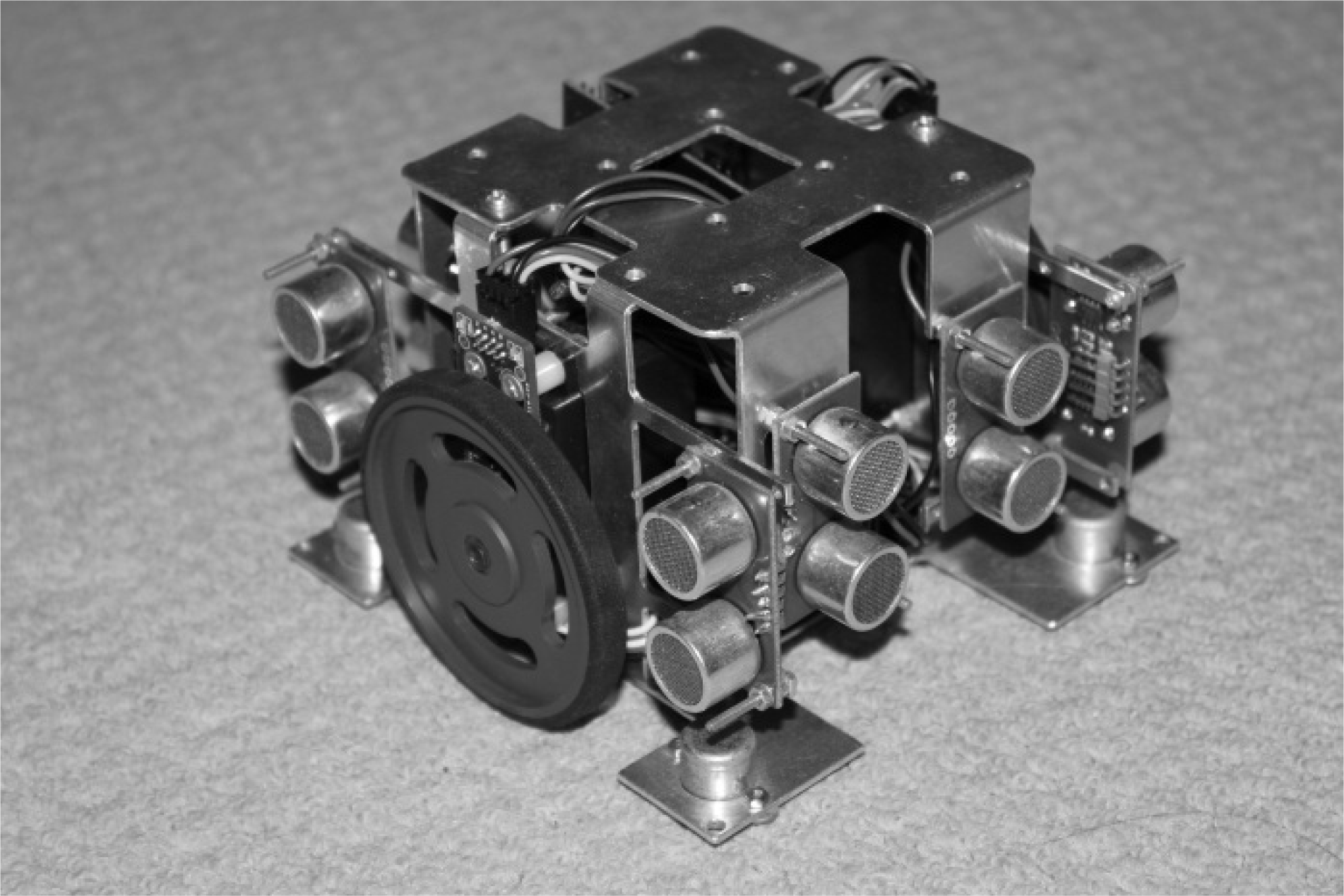
The KCLBOT [12] is a non-holonomic two wheeled autonomous maneuverable mobile robot. The mobile robot is built around the specifications for ‘Micromouse Robot’ and the ‘RoboCup’ competition. These specifications contribute to the mobile robot's form, factor and size. This mobile robot holds a complex electronic system to support on-line path planning, self-localization, and even SLAM, which is made possible by the on-board sensor array. The mobile robot is loaded with eight Robot-Electronics SRF05 ultrasonic rangers [13]. The drive system of the mobile robot is supported by Nubotics WC-132 WheelCommander Motion Controller [14] and two WW-01 WheelWatcher Encoders [14]. The motors for the mobile robot are modified continuous rotation servo motors; these are required for the WheelCommander Motion Controller. The rotation of the mobile robot is measured by the Robot-Electronics CMPS03 Compass Module [13].

The combination of hardware electronics and drive mechanics makes the KCLBOT, as represented in Fig. 2, an ideal platform for the self-localization methodology.

In the maneuverable classification of mobile robots [15], the vehicle is defined as being constrained to move in the vehicle's fixed heading angle. For the vehicle to change maneuver configuration, it needs to rotate about itself. As the vehicle traverses on a two-dimensional plane, both left and right wheels follow a path that moves around the instantaneous center of curvature at the same angle, which can be defined as, and thus the angular velocity of the left and right wheel rotation is deduced as follows:

Figure 2.

The KCLBOT: A Non-holonomic Maneuverable Mobile Robot.

{\dot{θ}}_{L} = ω (i c c_{r} - \frac{L}{2})

(1)

{\dot{θ}}_{R} = ω (i c c_{r} + \frac{L}{2})

(2)

where L is the distance between the centers of the two rotating wheels, and the parameter icc_r is the distance between the mid-point of the rotating wheels and the instantaneous center of curvature. Using the velocities (1) and (2) of the rotating left and rights wheels, ${\dot{θ}}_{L}$ and ${\dot{θ}}_{R}$ respectively the instantaneous center of curvature, icc_r and the curvature angle, ω, can be derived as follows:

i c c_{r} = \frac{L ({\dot{θ}}_{R} + {\dot{θ}}_{L})}{2 ({\dot{θ}}_{R} - {\dot{θ}}_{L})}

(3)

ω = \frac{({\dot{θ}}_{R} - {\dot{θ}}_{L})}{L}

(4)

Using (3) and (4), two singularities can be identified. When ${\dot{θ}}_{R} = {\dot{θ}}_{L}$ , the radius of instantaneous center of curvature, ice_r, tends towards infinity and this is the condition when the mobile robot is moving in a straight line. When ${\dot{θ}}_{R} = - {\dot{θ}}_{L} {\dot{θ}}_{R} = - {\dot{θ}}_{L}$ , the mobile robot is rotating about its own center, and the radius of instantaneous center of curvature, icc_r, is null.

When the wheels on the mobile robot rotate, the quadrature shaft encoder returns a counter tick value; the rotation direction of the rotating wheel is given by a positive or negative value returned by the encoder. Using the numbers of tick counts returned, the distance travelled by the rotating left and right wheel can be deduced in the following way:

d_{L} = \frac{L_{t i c k s} π D}{L_{r e s}}

(5)

d_{R} = \frac{R_{t i c k s} π D}{R_{r e s}}

(6)

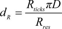
where L_ticks and R_ticks represent the number of encoder pulses counted by the left and right wheel encoders, respectively, since the last sampling and D is defined as the diameter of the wheels. With resolution of the left and right shaft encoders, L_res and R_res, respectively, it is possible to determine the distance travelled by the left and right rotating wheel, d_L and d_R. This calculation is shown in (5) and (6).

In the field of robotics, holonomicity [16] is demonstrated as the relationship between the controllable and total degrees of freedom of the mobile robot, as presented by the mobile robot configuration in Fig. 3. In this case, if the controllable degrees of freedom are equal to the total degrees of freedom, then the mobile robot is to be defined as holonomic. Otherwise, if the controllable degrees of freedom are less than the total degrees of freedom, it is non-holonomic. The maneuverable mobile robot has three degrees of freedom, which are its position in two axes and its orientation relative to a fixed heading angle. This individual holonomic constraint is based on the mobile robot's translation and rotation in the direction of the axis of symmetry and is represented as follows:

Figure 3.

The KCLBOT in X, Y, and Z Planar Environment.

{\dot{y}}_{c} \cos (φ) - {\dot{x}}_{c} \sin (φ) - d \dot{φ} = 0

(7)

where X_c and Y_c are Cartesian-based coordinates of the mobile robot's center of mass, and ϕ describes the heading angle of the mobile robot, which is referenced from the global x-axis. To conclude, (7) presents the pose of the mobile robot. The mobile robot has two controllable degrees of freedom, which control the rotational velocity of the left and right wheels and, adversely with changes in rotation, the heading angle of the mobile robot is affected. These constraints are as follows:

{\dot{y}}_{c} \sin (φ ​) + {\dot{x}}_{c} \cos (φ ​) + L φ = r {\dot{θ}}_{r}

(8)

{\dot{y}}_{c} \sin (φ ​) + {\dot{x}}_{c} \cos (φ ​) - L φ = r {\dot{θ}}_{l}

(9)

where ${\dot{θ}}_{r}$ and ${\dot{θ}}_{l}$ , are the angular displacements of the right and left mobile robot wheels, respectively, and where r describes the radius of the mobile robot's driving wheels. As such, the two-wheeled maneuverable mobile robot is a non-holonomic system. To conclude, (8) and (9) specify the angular velocity of the mobile robot's left and right wheels.

2.2 Self-Localization Using a Dual-Shaft Encoder Configuration

By using the quadrature shaft encoders that accumulate the distance travelled by the wheels, a form of position can be deduced by deriving the mobile robot's (x, y) Cartesian position and the maneuverable vehicle's orientation ϕ, with respect to time. The derivation starts by defining and considering s(t) and ϕ(t) to be function of time, which represents the velocity and orientation of the mobile robot, respectively. The velocity and orientation are derived from differentiating the position form as follows:

\frac{d x}{d t} = s (t) . \cos (φ (t))

(10)

\frac{d y}{d t} = s (t) . \sin (φ (t))

(11)

The change in orientation with respect to time is the angular velocity ω, which is defined in (4) and can be specified as follows:

\frac{d φ}{d t} = ω = \frac{{\dot{θ}}_{r} - {\dot{θ}}_{l}}{b}

(12)

When (12) is integrated, the mobile robot's angle orientation value ϕ(t) with respect to time is achieved. The mobile robot's initial angle of orientation ϕ(0) is written as ϕ₀ and is given as follows:

φ (t) = \frac{({\dot{θ}}_{r} - {\dot{θ}}_{l}) t}{b} + φ_{0}

(13)

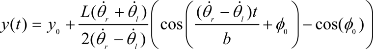
The velocity of the mobile robot is equal to the average speed of the two wheels and this can be incorporated into (10) and (11), as follows:

\frac{d x}{d t} = \frac{{\dot{θ}}_{r} + {\dot{θ}}_{l}}{2} \cos (φ (t))

(14)

\frac{d y}{d t} = \frac{{\dot{θ}}_{r} + {\dot{θ}}_{l}}{2} . \sin (φ (t))

(15)

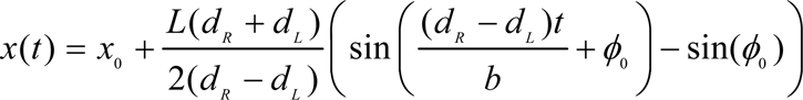
The next step is to integrate (14) and (15) to the initial position of the mobile robot, which is as follows:

x (t) = x_{0} + \frac{L ({\dot{θ}}_{r} + {\dot{θ}}_{l})}{2 ({\dot{θ}}_{r} - {\dot{θ}}_{l})} (\sin (\frac{({\dot{θ}}_{r} - {\dot{θ}}_{l}) t}{b} + φ_{0}) - \sin (φ_{0}))

(16)

y (t) = y_{0} + \frac{L ({\dot{θ}}_{r} + {\dot{θ}}_{l})}{2 ({\dot{θ}}_{r} - {\dot{θ}}_{l})} (\cos (\frac{({\dot{θ}}_{r} - {\dot{θ}}_{l}) t}{b} + φ_{0}) - \cos (φ_{0}))

(17)

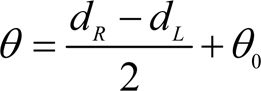
Equations (16) and (17) describe the mobile robot's position, where x(0) = x₀ and y(0) = y₀ are the mobile robot's initial positions. The next step is to represent (13), (16) and (17) in terms of the distances that the left and right wheels have traversed, which are defined by d_R and d_L. This can be achieved by substituting ${\dot{θ}}_{r}$ and ${\dot{θ}}_{l}$ in (13), (16) and (17) for d_R and d_L, respectively, and also dropping the time constant t to achieve the following:

θ = \frac{d_{R} - d_{L}}{2} + θ_{0}

(18)

x (t) = x_{0} + \frac{L (d_{R} + d_{L})}{2 (d_{R} - d_{L})} (\sin (\frac{(d_{R} - d_{L}) t}{b} + φ_{0}) - \sin (φ_{0}))

(19)

y (t) = y_{0} + \frac{L (d_{R} + d_{L})}{2 (d_{R} - d_{L})} (\cos (\frac{(d_{R} - d_{L}) t}{b} + φ_{0}) - \cos (φ_{0}))

(20)

Implementing (18), (19), and (20) provides a solution to the relative position of a maneuverable mobile robot. This is a possible solution to the self-localization problem but is subject to accumulative drift of the position and orientation with no method of re-alignment. The accuracy of this method is subject to the sampling rate of the data accumulation, such that if small position or orientation changes are not recorded, the position and orientation will be erroneous.

3. Navigation Environment Building Using a RGB-D Visual Sensor

3.1 A RGB-D Image Capture using Microsoft's Kinect™ Sensor

In early November 2010, Microsoft released the Kinect™ sensor, which has the capability of RGB and RGB-D image capture. Exploiting the pre-released drivers for this device, it is possible to export and manipulate both the RGB and RGB-D images for mapping, sensing, locating and modeling for SLAM.

The Kinect™ depicted in Fig. 4, which is mounted on the KCLBOT, is built around PrimeSense's PS1080 SoC [2]. The PS1080 acts as a controller for the IR light source in order to build the input image with IR light coding depth information. The light coding in this case is mapped on HSV [17]. The device is configured such that a standard CMOS image sensor receives the projected IR light source and transforms the image to produce a depth image. The sensor has a field of view of 58° Horizontal (H), 40° Vertical (V), and 70° Diagonal (D). The sensor allows for a maximum image depth size of VGA, which is a resolution of 640×480 and has maximum image throughput frame rate of 60fps. Finally, the operational range of the sensor is limited to a minimum of 0.8m and to a maximum of 3.5m.

Figure 4.

The Kinect™ Mounting Configuration on the KCLBOT.

As depicted in Fig. 5, the sensor is able to acquire RGB and RGB-D images, where the RGB-D images are used for environment building.

Figure 5.

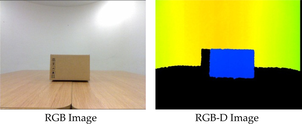
RGB and RGB-D Sensor Images.

3.2 Distance Estimation Using an RGB-D Sensor

Before the RGB-D images can be used for environment map building, the depth information from the image needs to be computed. To achieve this, a function needs to be derived to convert the RGB color values to Hue. Once the Hue value is acquired, it can be used to compute relative distance estimation. Using the model presented by Joblove and Greenberg [17], the following equation is implemented.

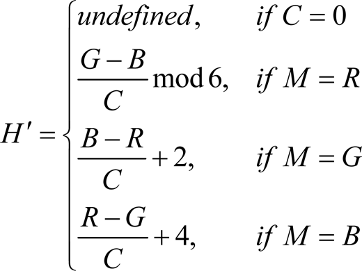
H^{'} = {\begin{array}{l} u n d e f i n e d, & i f C = 0 \\ \frac{G - B}{C} \mod 6, & i f M = R \\ \frac{B - R}{C} + 2, & i f M = G \\ \frac{R - G}{C} + 4, & i f M = B \end{array}

(21)

Here (21), the formula specifies the transpose of Hue value, using C = M − m, which specifies the chroma value and where M = max(R,G,B) and m = min(R,G,B) specify the maximum and minimum values of the RGB color, respectively.

The conversion function used to convert the transpose of Hue (21) to the Hue value needed, is as follows.

H = 60 ° . H^{'}

(22)

Now that a conversion for Hue from RGB has been defined, a function to convert the Hue values to distance is required. To achieve this, sample images are captured from the sensor, using a static object with a known distance from the sensor.

Using the images presented in Fig. 6, the average RGB values from the static object are extracted and converted to a Hue valuation.

Figure 6.

Sample RGB-D Distance Estimation Images.

The values required to build a Hue to distance function are presented in Table 1.

Table 1.

Sample RGB-D Distance Estimation Results

Sample	R	G	B	Hue	Distance (cm)
1	0	60	255	225.88°	81.67
2	2	162	255	202.06°	95.60
3	0	249	255	181.41°	110.60
4	0	255	31	127.29°	162.81

d = 0.0032 H^{2} - 1.9492 H + 359.26

(23)

Using Table 1, a distance estimation function is presented by (23).

Using the quadratic equation that describes distance as a function of Hue, a behavior graph is produced, and presented in Fig. 7. Based on this graph, when distance is less than 80cm or greater than 350cm, the slope of the curve changes more significantly. This conforms to the manufacturer's specifications on the limitations of distance estimation above and below these distance ranges.

Figure 7.

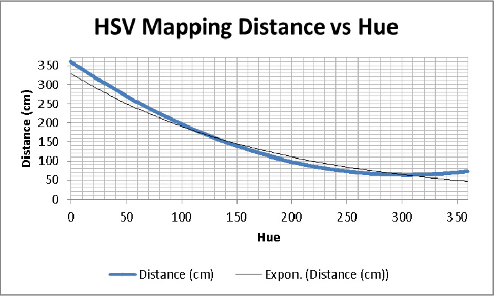
HSV Exponential Mapping of Distance vs. Hue.

3.3 Experiment Statistical Analysis

To validate the distance estimation equation presented in (23), the RGB-D sensor is used to capture 220 image samples of a static object between a distance range of 80 to 300cm, with sample steps on 1cm. This selection was made based on the behavior of the curve presented in Fig. 7. At the same time as the image is captured, an empirical measurement of distance is taken. The empirical measurement has a tolerance of 0.5mm error. The images are processed on the Microsoft .NET Micro Framework microcontroller and stored on a database on the microcontroller board, for analysis.

Table 2.
Statistical analysis of experimental data

Method Evaluation

Mean −0.06732103

95% Confidence Interval for Mean (LB) −0.09335622

95% Confidence Interval for Mean (UB) −0.04128584

5% Trimmed Mean −0.06671140

Median −0.05426171

Variance 0.022

Standard Deviation 0.147663453

Standard Error Mean 0.013154906

Minimum −0.390004

Maximum 0.197844

Range 0.587848

Interquartile Range 0.24780

Skewness −0.033

Kurtosis −0.933

Method	Evaluation
Mean	−0.06732103
95% Confidence Interval for Mean (LB)	−0.09335622
95% Confidence Interval for Mean (UB)	−0.04128584
5% Trimmed Mean	−0.06671140
Median	−0.05426171
Variance	0.022
Standard Deviation	0.147663453
Standard Error Mean	0.013154906
Minimum	−0.390004
Maximum	0.197844
Range	0.587848
Interquartile Range	0.24780
Skewness	−0.033
Kurtosis	−0.933

The results presented in Table 2 show statistical analyses of the 220 samples taken from the microcontroller. The mean value is relatively low and for more accuracy because the data might be skewed the median value is more useful and is comparably low. The confidence intervals which represents two standard deviations from the mean, equivalently present a low error rate.

The histogram in Fig 8 demonstrates that the error is roughly normally distributed between −0.3 to 0.2 and shows some anomaly below −0.3.

Figure 8.

The Frequency vs. Error Histogram

The boxplot presented in Figure 9 visually shows the distance from 0 to the mean, which is −0.067. It also presents the interquartile range, which is 0.248 and minimum (−0.39) and the maximum (0.198) values.

Figure 9.

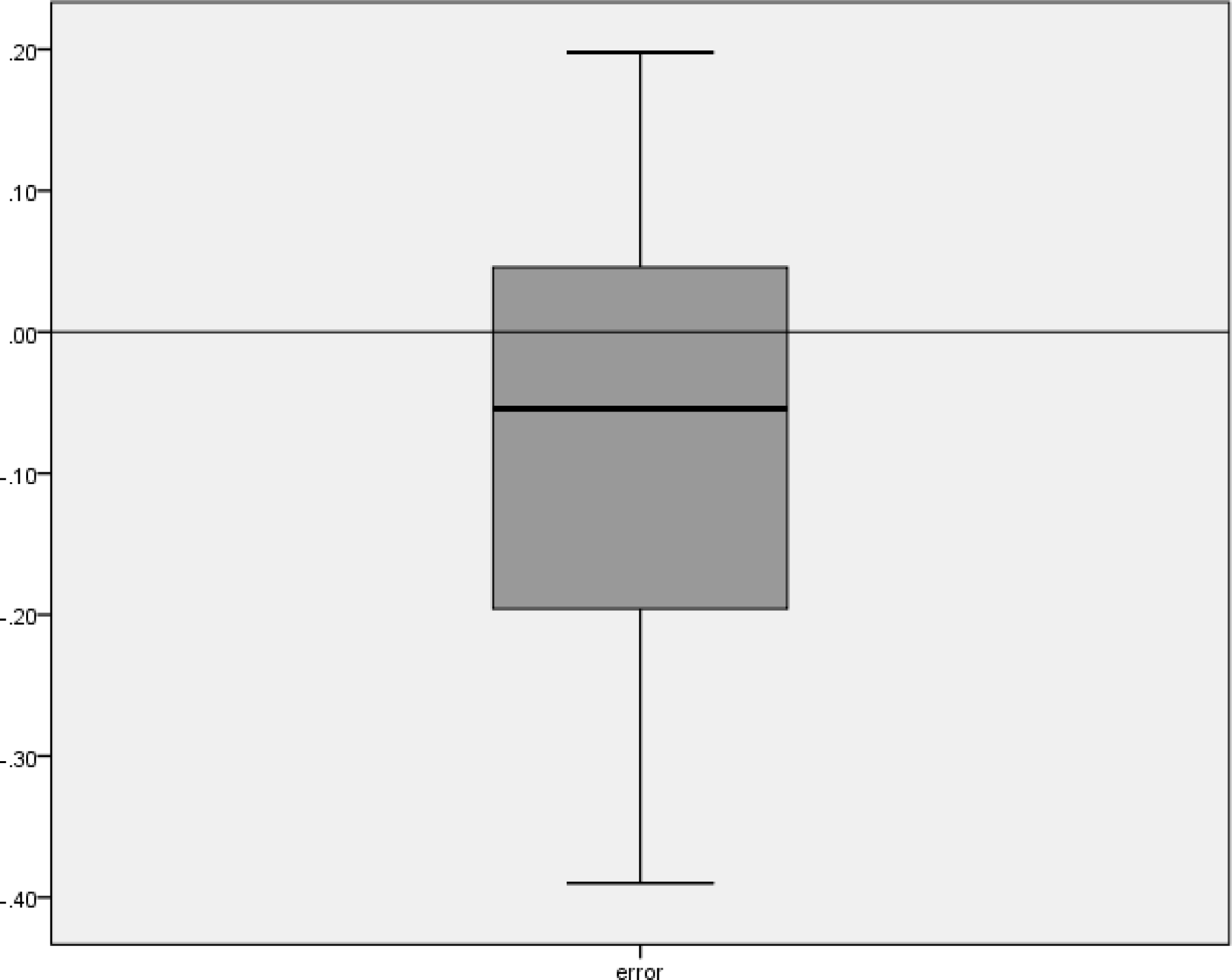
Boxplot of the experiment data

The Q-Q plot depicted in Figure 10 presents the performance of the observed values against the expected values. This demonstrates that the errors are approximately normally distributed centrally, with anomalies at both tail ends.

Figure 10.

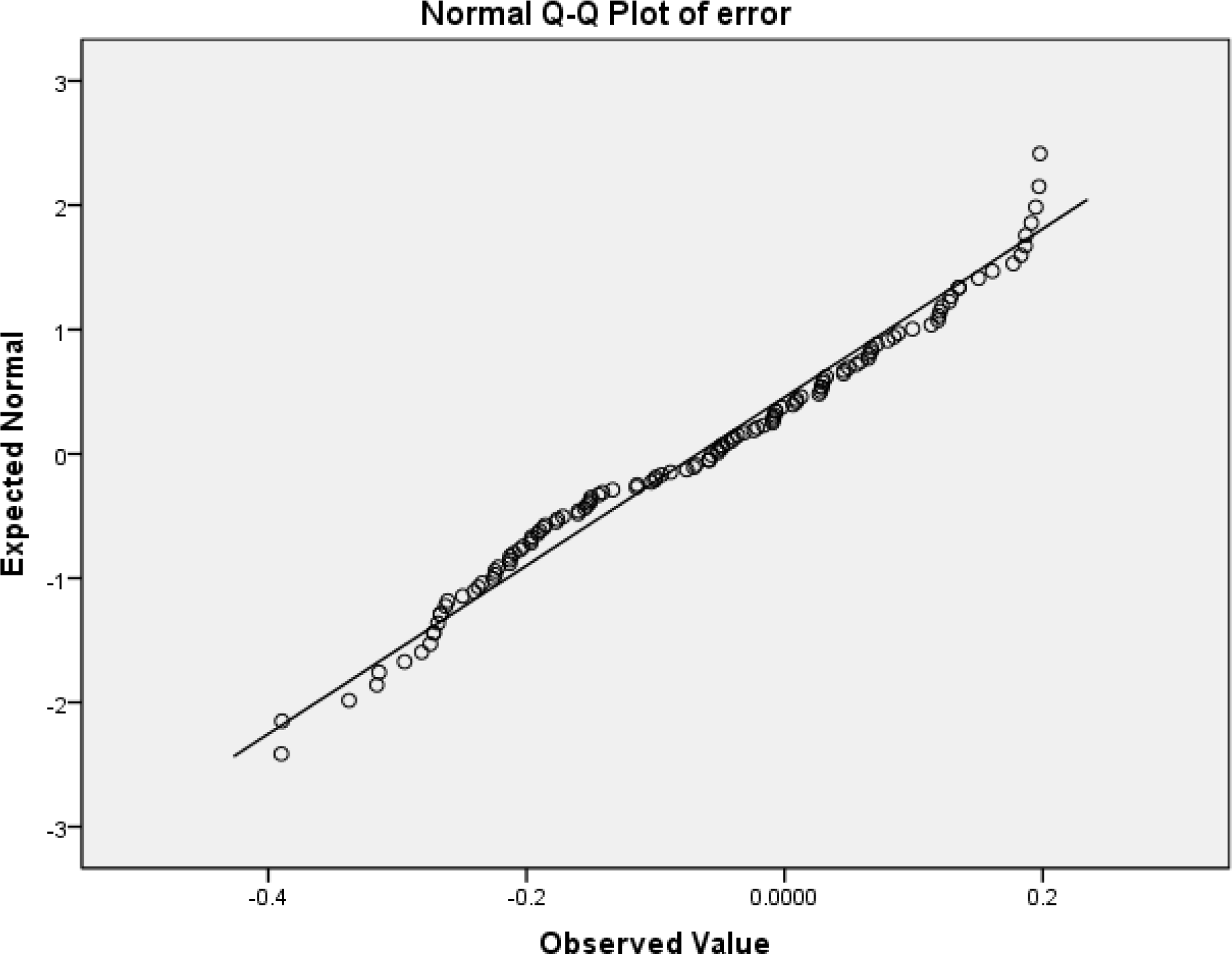
Normal Q-Q plot of error

3.4 Experiment Validation

Using the statistical analysis presented in the previous section, a non-parametric test is required to validate the practical effectiveness of the distance estimation equation (23). The ideal analysis test for a non-parametric independent one sample set of data is the Kolmogorov-Smirnov test [18] for significance.

The empirical distribution function F_n for n independent and identically distributed random variables observations X_i is defined as follows:

F_{n} (x) = \frac{1}{n} \sum_{i = 1}^{n} I_{X_{i} \leq x}

(24)

Where I _{X_ix} describes the indicator function, which is equal to 1 if X _t  X and is equal to 0 otherwise.

The Kolmogrov-Smirnov statistic [18] for a cumulative distribution function F(X) is as follows:

D_{n} = \sup_{x} | F_{n} (x) - F (x) |

(25)

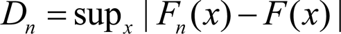
Where Sup_x describes the supremum of the set of distances. For the analysis test to be effective to be able to reject a null hypothesis, a relatively large number of data is required.

Under the null hypothesis that the sample originates from the hypothesized distribution F(X), the distribution is described as follows:

\sqrt{n} D_{n} \overset{n \to \infty}{\to} \sup_{t} | B (F (t)) |

(26)

Where B(t) describes the Brownian bridge [19].

If F is continuous, then under the null hypothesis √nD_n converges to the Kolmogorov distribution, which does not depend on F . The analysis test is constructed by using the critical values of the Kolmogorov distribution. The null hypothesis is rejected at level α if √nD_n > K _a, where K _a is calculated from the following:

\Pr (K \leq K_{a}) = 1 - α

(27)

It should also be noted that the asymptotic power of this analysis test is 1.

For the experimental data presented in this paper the null hypothesis is that the distribution of error is normal with a mean value of −0.06732 and a standard deviation of 0.14766. Based on significance level of 0.05, a significance of 0.44 is returned using the one sample Kolmogorov-Smirnov test (28). The strength of the returned significance value allows us to retain the null hypothesis and say that the distribution of error is normal with a mean value of −0.06732 and a standard deviation of 0.14766.

4. Environment Building

Before the autonomous mobile robot can complete any path planning or path following tasks, it requires sufficient information about the environment that it will be traversing. To provide the mobile robot with this information, the detail from the RGB-D camera is used to make a plot of the terrain, mapping the unobstructed space the mobile robot can utilize.

Before the RGB-D image can be used, the noise, resolved as black pixels in the range of #E4ElC0h to #FFFFFFh, needs to be removed from the image. This is achieved by converting the RGB-D image to gray scale [20]. This process is carried out to protect natural colors in the #E4ElC0h to #FFFFFFh range. In the RGB color model, a color image can be represented by the following intensity function:

I_{R G B} = (F_{R}, F_{G}, F_{B})

(29)

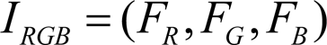
In (29), F_R is the intensity of the pixel (x,y) in the red channel, F_G is the intensity of pixel (x,y) in the green channel, and F_B is the intensity of pixel (x,y) in the blue channel. Using only the brightness information, the color image can be transformed into a gray scale image [20].

The equation that converts a color pixel to a gray scale pixel is presented below (25).

I_{G S} = 0.333 F_{R} + 0.5 F_{G} + 0.1666 F_{B}

(30)

After the image has been converted to gray scale, as depicted in Fig. 11, the black pixels are filtered out of the image.

Once the image has been stripped of the black noise pixels, as depicted in Fig. 12, the color detail is required for mapping the traversable environment.

The RGB-D depth color information from Fig. 11 is remapped onto the gray scale filtered image; the result is presented in Fig. 13.

Figure 11.

Conversion from RGB-D to Gray Scale.

Figure 12.

Conversion from RGB-D to Gray Scale.

Figure 13.

Remapping Color on Filtered Gray Scale Image.

R_{x} (θ) = [\begin{matrix} 1 & 0 & 0 \\ 0 & \cos (θ) & - \sin (θ) \\ 0 & \sin (θ) & \cos (θ) \end{matrix}]

(31)

O u t p u t_{p i x e l} = [\begin{matrix} x_{p i x e l} & R G B ​ - ​ D_{p i x e l} & - y_{p i x e l} \end{matrix}]

(32)

The input matrix (31) is multiplied by the rotation matrix [21] from (32), where θ = 90°, to produce a topological view of the traversable space.

O u t p u t_{p i x e l} = [\begin{matrix} x_{p i x e l} & R G B ​ - ​ D_{p i x e l} & - y_{p i x e l} \end{matrix}]

(33)

Using the first two components of (33), a 2-dimensional traversable space plot is produced, where the RGB–D_pixel is calculated using (23).

The generation of a topological view of the available navigation space, as presented in Fig. 14, provides the mobile robot with sufficient information for path planning and obstacle avoidance.

Figure 14.

Environment Map Generation from RGB-D Image.

Using a simple Bezier path [22], the KCLBOT is instructed to traverse a defined path and capture sample images using the RGB-D camera. Using the mobile robot's ability to self-localize, implementing (18), (19), and (20), while capturing and superimposing the converted images, using (33), an environment map is constructed.

The initial results presented in Fig. 15, provide the mobile robot with detailed information of the environment and it can easily estimate the Euclidean distance to all obstacles in range.

Figure 15.

Environment Map Generation from Path Following.

Using the depth information from equation (34) and mapping depth on the pixels of the image in Fig 13 it is possible to build a 3D reconstruction of the environment, which is demonstrated in Fig 16.

Figure 16.

Single sample 3D image reconstruction

5. Conclusion

The introduction of the affordable off-the-shelf RGB-D camera sensor, which captures images with depth information mapped in the HSV range, makes SLAM possible with minimal computation. This is validated by the experimental results presented in Fig. 11. The only concern of note at this stage is the tolerance levels presented by the distance estimation behavior graph in Fig. 6. The limitation is that obstacles 0.8m away from the sensor will not be resolved accurately. This is only a concern for navigation in small spaces but if the navigation area is large and open spaces are available, the sensor will prove to be a valuable tool for SLAM.

The experiment results and statistical analysis is valuable for anyone wanting to adopt a similar monocular sensor approach. The retention of the null hypothesis validates the use of the sensor and the performance is acceptable for small form factor mobile robots requiring environment mapping.

References

Thrun

, Learning Metric-Topological Maps for Indoor Mobile Robot Navigation. Journal on Artificial Intelligence, 1998. 99(1): p. 22–71.

Elfes

, Using Occupancy Grids for Mobile Robot Perception and Navigation. Computer Journal, 1989. 22(6): p. 47–57.

Leonard

Durrant-Whyte

, and Cox

, Dynamic Map Building for an Autonomous Mobile Robot. The International Journal of Robotic Research, 1992. 11: p. 286–298.

Fang

, and Dai

A Multi-Sensor Fusion SLAM Approach for Mobile Robots. in 2005 IEEE International Conference on Mechatronics and Automation. 2005.

Microsoft .NET Micro Framework. Available from: http://www.microsoft.com/en-us/netmf/default.aspx.

Windows Presentation Foundation (WPF).

Netdruino Plus. Available from: http://www.netduino.com/netduinoplus.

GHI ChipworkX Development System. Available from: http://www.ghielectronics.com/catalog/product/125.

OpenKinect. Available from: http://www.openkinect.org.

10.

Robot Operating System (ROS). Available from: http://www.ros.org.

11.

Chilian

, and Hirschmuller

Stereo camera based navigation of mobile robots on rough terrain. in International Conference on Intelligent Robots and Systems.

12.

Georgiou

KCLBOT. 2010; Available from: http://www.kclbot.com.

13.

Mobile Robot Distance & Orientation Sensors. Available from: http://www.robot-electronics.co.uk.

14.

Mobile Robot Navigation Sensors.

15.

Campion

Bastin

, and D'Andrea-Novel

, Structural Properties and Classification of Kinematic and Dynamic Models of Wheeled Mobile Robots. IEEE Transactions on Robotics and Automation, 1996. 12(1).

16.

Kolmanovsky

I.a.M. N.

, Developments in nonholonomic control problems. IEEE Control Systems Magazine, 1995: p. 20–36.

17.

Joblove

, and Greenberg

Color spaces for computer graphics. in 5th Annual Conference on Computer Graphics and Interactive Techniques.

18.

Zhang

Wang

Liang

, and Li

, Fast and Robust Spectrum Sensing via Kolmogorov-Smirnov Tes. IEEE TRANSACTIONS ON COMMUNICATIONS, 2010. 58(12): p. 3410–3416.

19.

Zhu

, Bounded Brownian bridge model for UWB indoor multipath channel, in IEEE International Symposium on Microwave, Antenna, Propagation and EMC Technologies for Wireless Communications, 2005. MAPE 2005. 2005. p. 1411–1414.

20.

Kumar

, and Verma

, A Theory Based on Conversion of RGB image to Gray image. International Journal of Computer Applications, 2010. 7(2): p. 7–10.

21.

Herter

, and Lott

, Algorithms for decomposing 3-D orthogonal matrices into primitive rotations. Journal on Computers & Graphics, 1993. 17(5): p. 517–527.

22.

Choi

Curry

, and Elkaim

Path Planning Based on Bézier Curve for Autonomous Ground Vehicles. in Proceedings of the Advances in Electrical and Electronics. 2008.