Sage Journals: Discover world-class research

Abstract

Exact computation of the shape and size of robot manipulator workspace is very important for its analysis and optimum design. First, the drawbacks of the previous methods based on Monte Carlo are pointed out in the paper, and then improved strategies are presented systematically. In order to obtain more accurate boundary points of two-dimensional (2D) robot workspace, the Beta distribution is adopted to generate random variables of robot joints. And then, the area of workspace is acquired by computing the area of the polygon what is a closed path by connecting the boundary points together. For comparing the errors of workspaces which are generated by the previous and the improved method from shape and size, one planar robot manipulator is taken as example. A spatial robot manipulator is used to illustrate that the methods can be used not only on planar robot manipulator, but also on the spatial. The optimal parameters are proposed in the paper to computer the shape and size of 2D and 3D workspace. Finally, we provided the computation time and discussed the generation of 3D workspace which is based on 3D reconstruction from the boundary points.

Keywords

Beta distribution Robot manipulator Polygon area 2D and 3D workspace Shape and size

1. Introduction

The workspace of robot manipulator is defined as the set of points that can be reached by its end-effector. The workspace of conventional robots has been studied for more than three decades and many methods have been proposed. In the computation of robot workspace, what we most concerned is its corresponding shape and size. The boundary curves (for 2D robot manipulators) and surfaces (for 3D robot manipulators) of robot workspace have been studied using graphical, analytical or numerical methods.

The theorem that the robot manipulator is in a singular configuration when it reaches the workspace boundaries was proved in [1]. Based on this theorem, several analytical criteria for determining the workspaces' boundaries were derived in [2-10]. In a series of articles [4,5,11-13], a set of analytical criteria for determining workspace boundaries of parallel manipulators were presented and employed continuation method to map the boundary curves. Kumar and Waldron [14] used reciprocal screws to describe the boundary surface of manipulator's workspace. Sugimoto and Duffy [15,16] proposed a theorem for extreme distances of manipulators and based on this theorem to search for the manipulator's extreme reaches. Freudenstein and Primrose [17] introduced skew-torus geometry to determine the workspace's boundaries of a three-link mechanism. Some optimization based algorithms were proposed in [18, 19] to generate the boundary's profile and workspace volume. Castelli et al. [20] proposed a general boundary-computation algorithm based on the binary representations of the manipulator workspaces. The workspace of a space manipulator was studied in [21] using the conventional analytic or geometric method based on the concept of ‘Virtual Manipulator'. The convolution product of real-valued functions on the Special Euclidean group (which in fact is a discretized one), was introduced to determine workspaces which have a finite number of joint states [22]. A diffusion-based algorithm was developed for the workspace of snake-like hyper-redundant robots in [23] and related work. There are also some other approaches [24–32] which utilized the geometric properties of the motion trajectories. Thus, efficient and comprehensive methods in the literature for determining the workspace boundary and its expression of size or volume require analytic expressions for inverse kinematics, which are often not available or require specialized methodologies, especially for 3D workspace.

The Monte Carlo method is a numerical method for solving mathematical problems by means of random sampling. Since the Monte Carlo method involves no inverse Jacobian calculation, is relatively simple to apply and has been used by many investigators to generate workspace boundary and the corresponding size [33-41]. Unfortunately, most of these works can only determine workspace boundary curves for 2D manipulators [33-36, 38, 39]. Although the optimization-based method and the Monte Carlo method were used in [37] to generate workspace in 3D, the volume of workspace was not involved. In a series of papers [40, 41], we used Monte Carlo method and some commercial softwares to generate 3D shape and volume of spatial robot workspace. In [40], the planar boundary curve of spatial robot in its main working plane is depicted and then 3D workspace are generated by revolving the boundary curves around an axis within Unigraphics. To improve the method presented in [40] to suit more complex robot manipulators, we depict the boundary curves in a series of slices, and generate the workspace by solid modeling method within Solidworks [41]. However, the method [41] should use two different softwares so has to satisfy the data consistency and need cost much extra time in operating these commercial softwares. Hence, the client should understand not only the computing softwares, such as Matlab, Visual C++, but also 3D engineering softwares. The case is very inconvenient for mechanism design and synthesis of robot manipulator. Therefore, it is necessary to propose a systematical method to fast and accurate compute the shape and size of 2D and 3D workspace in one software.

The organization of the paper is as follows: in the second section, two robot manipulators are illustrated and the kinematics is formulated. The features, especially the drawbacks of the previous methods are analyzed in Section three. In the next section, an algorithm using Beta random distribution for the joint variable is adopted to obtain a more accurate boundary curve. In Section five, we estimate the area of workspace by treat boundary curve as a polygon. We use trapezoidal-based numerical integration to calculate the volume of a 3D robot workspace in Section 6. We provide the elapsed time in computing the 2D and 3D workspace, and discuss results with possible extension of the systematical method in Section 7, and finally draw conclusions in Section 8.

2. Two illustrative examples

In the paper, two robot manipulators are used to illustrate the systematical method.

Figure 1.

3R planar robot manipulator

A planar robot manipulator consisting of three links and three revolute joints (J1, J2 and J3) (3R planar example) is shown in Fig. 1. The kinematics of the robot manipulator can be obtained in the coordinates OXY by Denavit–Hartenberg [42].

{\begin{cases} x = l_{1} c_{1} + l_{2} c_{12} + l_{3} c_{123} \\ y = l_{1} s_{1} + l_{2} s_{12} + l_{3} s_{123} \end{cases}

(1)

where c and s denote cosine and sine, respectively, c₁₂ is cos (θ₁+θ₂) in short.

Figure 2.

3R spatial robot manipulator

The position vector of the end-effector p is a mapping from the n-dimension (n is 3 in the example) joint variable space to the workspace of the end-effector. Generally speaking, a robot manipulator has physical constraints on its joint motion range. The joint can not move exceed their limits. Denote $\underline{θ}$ and $\bar{θ}$ the lower and upper bounds of the joint limits, respectively, then the joint limit is $θ \in [\underline{θ}, \bar{θ}]$ . For the example, the joints limits are $θ_{1} \in [- 2 π / 3, 2 π / 3]$ , and $θ_{2} = θ_{3} \in [- π / 3, π / 3]$ , respectively. Also, l₁ = 4, l₂ = 2, and l₃ = 1 (in unit length).

A spatial robot manipulator is shown in Fig. 2, which include three revolute joints too (3R spatial robot example). Forward kinematics of the robot manipulator is

{\begin{cases} x = c_{1} (l_{2} c_{2} + l_{3} s_{23}) \\ y = s_{1} (l_{2} c_{2} + l_{3} s_{23}) \\ z = l_{1} + l_{2} s_{2} - l_{3} c_{23} \end{cases}

(2)

where the motion ranges of the three revolute joints are $θ_{1} = θ_{2} = θ_{3} \in [- π / 2, π / 2]$ . Also, the lengths of all linkers are l₁=l₂= l₃=1.

3. Features of the previous method

In [38], a numerical method based on Monte Carlo was used to obtain the shape and size of workspace. The method is simple to depict the workspace boundary from engineering standpoints. However, as pointed out by [39], in some cases, the method will result in errors in computing workspaces. Consequently, an improved approach searching for the boundary from two axes is presented in [39], which increases the number of boundary points by searching boundary points from two coordinate-axises and avoids obtaining a wrong contour.

Figure 3.

Boundary curves of 3R planar robot manipulator

The improved method [39] has another merit, which can tell whether there are holes in the workspace. For example, after obtaining the boundary points, the nearest points should be connected one by one from an extreme point by straight line segments. If the distance of two neighbor points is too large (e.g. 5 times to the column width), shows that there are holes in the workspace.

However, in recent study, we found that in some cases, the workspace shape generated by the improved approach is not accurate enough. Fig. 3 is the workspace boundary curve of 3R planar robot with 30,000 random points and 40-by-40 sliced columns in searching boundary points. We can find that the curve segments P1P2P3, P3P4 and P6P1 are not smooth, while the curve segment P4P5P6 is relatively smooth. This deviation will negatively influence not only the shape, but also the area estimation of workspace. So, we continue to improve the method in [39], to acquire a more accurate shape.

4. A Beta-distribution based method

4.1. Distribution characteristics of Monte Carlo points in workspace

The position of end-effector p with respect to world frame can be simply calculated by the forward kinematics of robot. As we can see from the kinematics Equation (1) and (2), the position of the reference point in workspace is a nonlinear and transcendental function of the related joint angles. In the previous method, we produced a number of random values for every joint, whose elements are uniformly distributed in their motion range. However, the mapping points in workspace are not uniformly distributed from the forward kinematics of robot manipulator. Fig. 4 is the workspace of the 3R planar robot manipulator. We generate 6000 random numbers with uniform distribution for the revolute joints. The densities of the Monte Carlo points (or as point cloud) are not uniform in workspace what we can observe by eyes. In order to improve the accuracy of workspace boundary, we should know the density distribution of Monte Carlo points and then analyze the reasons causing such problems.

Figure 4.

Distribution of Monte Carlo points in planar workspace

For calculating the probability density, we define the term of Density of Monte Carlo points as the number of reachable points per unit workspace volume, where the workspace is discretized into small blocks. In order to discretize the workspace into small blocks, we should firstly find an envelope rectangle to contain the workspace. And then, bins the elements of the points into an n-by-n grid of equally-spaced containers, i.e. blocks. The detailed steps are:

Figure 5.

Envelope rectangle of the workspace

Figure 6.

Density distribution of Monte Carlo point cloud

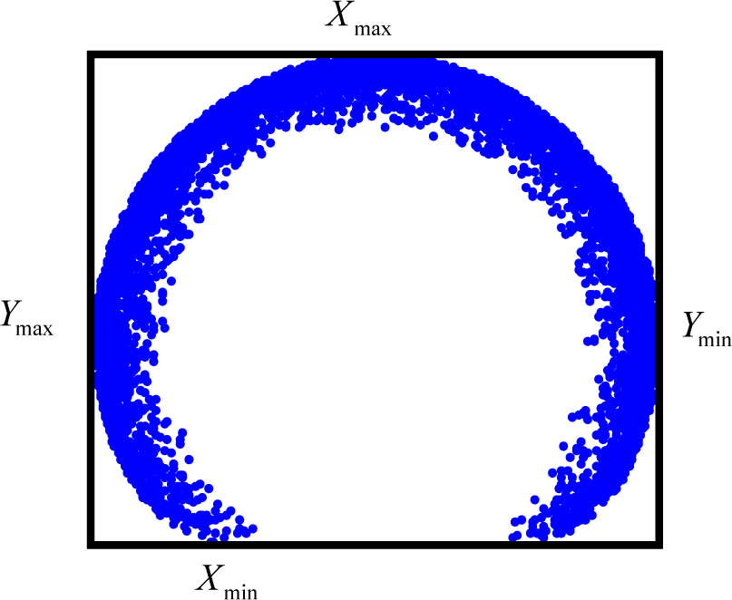
Firstly, search for the extreme values Ymax, Ymin along Y-axis and Xmax, Xmin along X-axis in the boundary points. There are four points corresponding to the four values, respectively. We draw four line segments through the fours points parallel to X-axis or Y-axis respectivlly, which construct a rectangle, shown in Fig. 5. This is an envelope rectangle containing the workspace.

Secondly, we bin the workspace points into an n-by-n grid of equally-spaced blocks, where the n is determined by the desired accuracy.

Thirdly, the number of the points in each block is calculated by the three -dimensional histogram shown in Fig. 6, where X and Y denote the coordinates of each block and Z (height of histogram) means the point number in the block.

We can roughly estimate the density of point of one block in workspace by the following equation:

ρ_{D} = \frac{Z (Height of histogram)}{Gross number of point cloud} \times 100 %

(3)

Another way for investigating the distribution of point cloud in workspace is contour plot. By the forementioned steps, we can obtain the contour plot of point density in workspace, shown in Fig. 7, where the plot is provided with 3 contour levels. As we can see, the workspace is something like a letter “C”. The regions with the highest density are depicted by the solid lines, which appear in the inner of the workspace. The region enclosed by dashed lines is the lowest density contour, which occur at the boundary of the workspace. Due to most of the Monte Carlo points concentrate on the inner of workspace rather than the boundary, the distribution of these points on the boundary is sparse. The situation results in that there are not enough points approaching the true workspace boundary. That is to say, it is difficult to get the precise boundary points of the workspace. Once the obtained boundary points are connected to generate the boundary curves, the curves are not smooth. Although we can increase the random numbers of joint variable, most of the points are still mapped at the highest density regions rather than the boundary. On the other hand, the augmented points in workspace lead to the rapid increase in computation time.

Figure 7.

Contour plot of point cloud density in workspace

4.2. Probability density distribution of manipulator joints variables

After analyzing the contour plot, we found that the joints ranges corresponding to the regions with sparse points are the lower and/or upper bounds of the joint variables. Corresponding to the boundary curves (see Fig. 3), such as P1P2P3, P3P4 and P6P1, at least one joint of robot manipulators reached its lower or upper bounds, i.e. kinematics limits. For example, three joints reach their limits at the corner P1 and P3, and the J2 and J3 reach their limits at the boundary curve P1P2P3. Consequently, we have to take some other distribution functions for joint variable which can mapping more points to the boundary parts. The new distribution function should have such features that its density function or its shape can be adjusted by changing some parameters. For this issue, we hope more random numbers of each joint variable appear at the lower and upper bounds in its range. Based on such considerations, the Beta distribution function is chosen for improving the algorithm [43].

4.3. Beta Distribution and determination of parameters

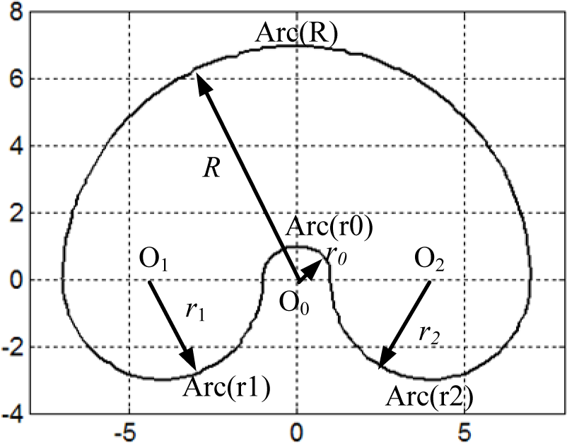
The Beta density function is a very versatile way to represent outcomes like proportions or probabilities. The standard Beta distribution gives the probability density of a value x on the interval (0,1):

B e t a (α, β) : p r o b (x | α, β) = \frac{x^{α - 1} {(1 - x)}^{β - 1}}{B (α, β)}

(4)

where B is the beta function

B (α, β) = \int_{0}^{1} t^{α - 1} {(1 - t)}^{β - 1} d t

(5)

One advantage of the Beta distribution is that it can take on many different shapes. The shape of the beta distribution is quite variable depending on the values of the parameters α and β, as illustrated by the Fig. 8. The constant probability distribution function (the flat line) shows that the standard uniform distribution is a special case of the Beta distribution.

Figure 8.

Shape of the beta distribution with different parameters

After adopting the Beta random distribution for joint variables to generate workspace, the next issue of which should be taken account is the ranges of α and β. For illustrating the issue, we suppose that the motion range of joints in the 3R planar manipulator work in two different ranges respectively. The first case is $θ_{1} = θ_{2} = θ_{3} \in [- π / 4, π / 4]$ , and the second is $θ_{1} = θ_{2} = θ_{3} \in [- 3 π / 4, 3 π / 4]$ . We still use uniform random distribution for these joints, and the number of random points is 6,000.

Figure 9(a).

Distribution of point cloud of the first case

Figure 9(b).

Distribution of point cloud of the second case

The distributions of point cloud of two cases are plot in Fig.9 (a) and Fig.9 (b). We can see clearly from the dual figures, that the density distributions of point cloud are different, especially at the part approaching lower boundary P1P2P3. According to Equation (3), the density of point cloud at the lower boundary P1P2P3 for the first case in less than 0.04%, while the density for the second one is about 0.07%. It can be concluded that the distribution of point cloud depend largely on the motion ranges of joints. What is more, from Fig.4 and Fig.9, the less of the motion ranges of joints, the more sparse of the point cloud on the lower boundary P1P2P3 and the corners, i.e. P1 and P3. Based on the above reasons, for getting higher point density at the workspace boundary, we choose both parameters α and β as bellow:

0 < (α_{i} = β_{i}) \leq 1 \begin{matrix} i = 1, 2, \dots, n \end{matrix}

(6)

where the i denote the ith joint of robot manipulators.

From our experiments, with respect to the motion range of joint variable, α and β can be determined by the following equations:

{\begin{cases} α_{i} = β_{i} = 0.4, 0 < ϑ_{i} < \frac{π}{2} \\ α_{i} = β_{i} = ϑ_{i} / 5 π + 0.3, \frac{π}{2} \leq ϑ_{i} < π \\ α_{i} = β_{i} = 3 ϑ_{i} / 5 π - 0.1, π \leq ϑ_{i} < \frac{3 π}{2} \\ α_{i} = β_{i} = 2 ϑ_{i} / 5 π + 0.2, \frac{3 π}{2} \leq ϑ_{i} \leq 2 π \end{cases}

(7)

where the $ϑ_{i}$ is the difference between the upper and the lower values of the ith joint limit, which can be formulated as

ϑ_{i} = \bar{θ_{i}} - {\underline{θ}}_{i}

(8)

For the 3R planar manipulator, we use the Beta random distribution for joint variables respectively to generate point cloud in workspace, which are shown in Fig.10, where the random number of each joints is 6000. Comparing the Fig.4 and Fig.10, we can find that more points are mapped approaching the workspace boundary in Fig.10, especially on P3P4, P6P1 and P1P2P3. Also, the distribution density of point cloud can be institutively observed from its corresponding contour plot shown in Fig.11. Furthermore, according to the contour plot in Fig.11, the density ratio of regions with the highest point density to the regions on the boundary is about 7 for Beta distribution, while the ratio is 13 for uniform distribution in Fig.7.

Figure 10.

Distribution of point cloud with Beta distribution

Figure 11.

Contour plot of point cloud with Beta distribution

We use 30,000 sets of random numbers from the Beta distribution of Equation (7) to formulate the joint variables of 3R planar robot manipulator. The boundary curve shown in Fig.12 is obtained from searching the boundary points and connecting them to construct a closed polygon. The number of rows and columns are 40, which is same to the example mentioned in Section 3. We can see in Fig.12, the boundary curve is smooth. Especially in the curve segment P1P2P3, it is almost impossible to find roughs or noises. We can use a circle fitting method [51] to quantitatively compare the accuracy of the arc segments P1P2P3 between Fig.3 and Fig.12. Note that, the center of the arc is (0, 0), and the radius is 5.2 in theory. By the circle fitting method, the center is (−0.0168, 0.0088), the radius is 5.337, and the max distance error from the boundary point to the radius is 0.1744 in Fig.3. While the center is (−0.0006, −0.0032), the radius is 5.233, and the max distance error is 0.1231 in Fig.12. Obviously, using the Beta distribution for generating random values of the robot's joints gives better results in workspace generation than when the uniform distribution is used.

Figure 12.

Boundary curve of workspace with Beta distribution

5. Area computation of robot workspace based on polygon

5.1. Algorithm description

In [38], a numerical integration method was proposed to calculate the area of planar robot workspace. In the method, the workspace is partitioned into a series of rectangles, and then sum all the rectangle areas. The method is simple to understand, however, it will lead to relatively big error in some conditions.

Figure 13.

Area estimation with rectangle

For Fig.13, in the row AA*, due to the boundary points are at the extreme positions along X-axis, the area of the rectangle covering the sub-workspace is usually larger than its actual size. Furthermore, such error will gradually grow along with the increasing absolute value of slope of the boundary curve.

Therefore, we need a more accurate method to calculate the workspace area. As aforementioned, the workspace boundary curve is composed of a series of line segments by connecting the boundary points. In fact, these line segments construct (a) closed polygon (s). In geometry, a polygon is a plane figure that is bounded by a closed path, composed of a finite sequence of straight line segments. These segments are called its edges or sides, and the points where two edges meet are the polygon's vertices or corners. An n-gon is a polygon with n sides. For robot workspace, the vertices of the polygon consist of the boundary points. To calculate the area of robot workspace is to compute the size of its corresponding polygon.

Supposed a polygon made up of line segments between N vertices (x_i,y_i), i=1 to N+1. The last vertex (x_N+1,y_N+1) is assumed to be the same as the first, i.e. the polygon is closed. Fig.14 is a schematic diagram of polygon with 6 vertices.

Figure 14.

Schematic diagram of a polygon

The area is given by the following equation [44]:

A_{w} = \frac{1}{2} \sum_{i = 1}^{N} (x_{i} y_{i + 1} - x_{i + 1} y_{i})

(9)

Note that the equation is established only for a non-self-intersecting (simple) polygon with n vertices.

In addition, the workspace with holes should be taken into account which corresponds to polygons with holes. In the condition, we determine the sign to the bounding polygon area is positive, while the holes areas are negative. That is, the holes areas will be of opposite sign to the bounding polygon area. The actual area is the algebra sum of the both.

5.2. Error comparison

In order to the comparing the accuracy on area computation resulted from two methods, the Percent Error Formula is used to calculate how far we have gone from our experimental value to the theoretical value. The equation can be described as

Percent Error = \frac{Experiment value-theoretical value}{Theoretical value} \times 100 %

(10)

where the Experiment value is the area size of computing result from our Monte Carlo method; the theoretical value is the actual area by analytical method from its geometry.

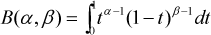
It is not an easy work to calculate the workspace area of the 3R planar manipulator, because the boundary curve consist of several arcs and the analytical expression is difficult to describe. For simplicity—but without loss of generality, the motion range of joints in the 3R planar manipulator are modified as $θ_{1} \in [- π / 2, π / 2]$ , and $θ_{2} = θ_{3} \in [- π, π]$ , respectively. The corresponding workspace is shown in Fig. 15.

Figure 15.

Boundary curve of planar manipulator with modified joint variables

The boundary curve consists of four half circular arcs (Arc (r0), Arc (r1), Arc (r2) and Arc (R)), the centre of each arc is marked in the figure (O₀, O₁ and O₂), and the equations of the four arcs are followed:

Arc (r0) : x^{2} + y^{2} = r_{0}^{2} = 1

(11.a)

Arc (R) : x^{2} + y^{2} = R^{2} =^{72} = 49

(11.b)

Arc (r1) : {(x + 4)}^{2} + y^{2} = r_{1}^{2} =^{32} = 9

(11.c)

Arc (r0) : {(x - 4)}^{2} + y^{2} = r_{1}^{2} =^{32} = 9

(11.d)

According to Equation (11), the area can be easily computed by the following equation:

A_{T} = \frac{1}{2} π (R^{2} + r_{1}^{2} + r_{2}^{2} - r_{0}^{2})

(12)

Substituting the radius of each arc into Equation (12), the area is about 103.67 which is the theoretical value.

We use Equation (10) to calculate percent error of area

E_{a} = \frac{A_{c} - A_{T}}{A_{T}} \times 100 %

(13)

where the A_c is experimental estimated value.

In Table 1, the percent errors E_a with different column number and different Monte Carlo points are listed, where the values in parentheses are resulted from the numerical integration based on rectangles. Each value in the table is the average after 5 calculations.

All the values in Table 1 calculated by Equation (9) and Equation (13) (outside of parentheses) are negative. This is due to the boundary points obtained from the numerical method, are not “on” the boundary, but approaching the boundary from workspace inner. In other words, the depicted boundary curve is not the actual boundary in geometric theory, but less than the actual boundary, because of all the point cloud only fall into the inner of workspace. Consequently, the corresponding area calculated by polygon area is smaller than the actual value. Besides, with the increase of point cloud, the absolute values of error in each column decrease gradually. For the data in each row, with the growth of sliced column in workspace (through 30 to 70), the changes of errors are not obvious. That is to say, the errors are stable in each row. The smallest errors in each row usually appear in the second column (such as −0.764 and −0.536) or the third column (such as −1.838 and −1.033). The minimum error appears in row 4, column 2 with 100,000 point cloud and 40 sliced columns in workspace.

Table 1.

Percent errors E_a of two methods

		Number of column (sliced in workspace)
		30	40	50	60	70
Number of point cloud (thousand)	10	−2.201 (2.074)	−1.853 (1.087)	−1.838 (0.186)	−2.378 (−0.657)	−2.673 (−1.255)
	30	−1.101 (3.486)	−1.592 (1.72)	−1.033 (1.534)	−1.158 (1.189)	−1.25 (0.437)
	50	−0.793 (3.87)	−0.764 (2.923)	−0.879 (2.073)	−0.841 (1.257)	−0.845 (1.116)
	100	−0.634 (4.305)	−0.536 (3.33)	−0.581 (2.35)	−0.588 (1.79)	−0.613 (1.374)

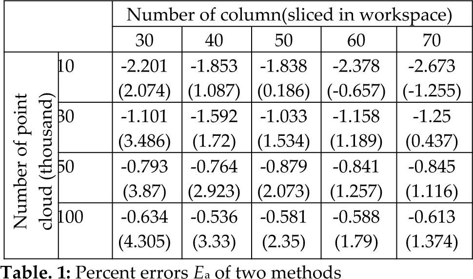
Different from above, most of the values in the table from numerical integration [38] (in parentheses) are positive. The reasons leading to the result have been analyzed in section 5.1 and by Fig.13. On the other hand, if the number of point cloud is not enough relative to the number of column, the obtained boundary points are far away from the actual boundary, so the estimated area is less than the actual value, just as listed in row 1, column 4 and column 5 in Table 1. Moreover, along with the increase of point cloud, the absolute values of error in each column are ascending except the last column, what is unacceptable for us. Nevertheless, with the growth of sliced column in workspace, the errors are decrease progressively in each row but the first row. The minimum error in parentheses appears in row 2, column 5 with 30,000 point cloud and 70 sliced columns in workspace.

In most cases in the table, the errors outside of parentheses is less than the corresponding errors in parentheses, but the data in the first row and the data in row 2 column 5. From engineering viewpoint, 20,000 to 30,000 point cloud and 40 sliced columns can satisfy accuracy requirement in most cases.

6. Boundary curves of 3D robot manipulator and volume calculation

6.1. Depicting boundary curves of 3D robot manipulator

Unlike the Monte Carlo method used in 2D workspace, it is difficult to be aware of the shape of 3D robot workspace from the point cloud which is obtained from robot manipulator kinematics, shown in Fig.16. Therefore, if we could get some boundary curves (envelope curves) of 3D workspace, it will help us to know the shape roughly.

Figure 16.

Point cloud of 3D workspace

The boundary curves in different slices of the 3D workspace can be depicted by the method proposed in [41]. In the paper, the difference is that we use Beta random distribution to the joint space of the manipulator to approximate the workspace. After obtaining the maxima Z_max and minima Z_min along the Z-axis in the point cloud, we uniformly slice the point cloud of workspace by using a series of horizontal planes along the Z direction with a reasonable resolution. The height of each slice is

ℏ = (z_{\max} - z_{m i i n}) / s

(14)

where s is the number of slices.

On each horizontal plane, we depict the boundary points and then boundary curve by connecting the points together.

By the above steps, the boundary curve of each slice can be acquired. As shown in Fig.17, all the boundary curves of slices can be viewed as a series of contours enveloping the robot workspace.

6.2. Volume calculation

Estimation of volume from serial sections typically involves using a rectangular, Cavalieri's, parabolic (Simpson's), or a trapezoidal rule to integrate numerically a curve of cross-sectional area measurements plotted against section number [45]. In this paper, we adopt the trapezoidal method by taking the accuracy and speed into account.

Figure 17.

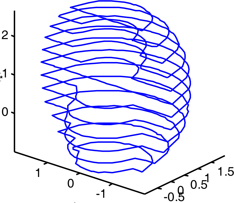
Envelope curves in different slices

The trapezoidal estimate of morphometric volume for equally spaced sections is determined by the following formula

V_{T} = d [\sum_{j = 1}^{s} A_{w j} - \frac{1}{2} (A_{w 1} + A_{w s})]

(15)

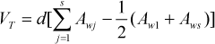
where d is the distance between the neighbour sections, $d = ℏ$ in value; A_wj (j=1 to n) stands for cross sectional area of the ith section through the morphometric region, and s is same to ‘s' in Equation (14).

The area of each slice can be calculated by Equation (9). Substituting Equation (9) and (14) into equation (15), gives the final equation of calculating volume.

\begin{array}{l} V_{T} = ℏ {\frac{1}{2} \sum_{j = 1}^{s} \sum_{i = 1}^{N} {(x_{i} y_{i + 1} - x_{i + 1} y_{i})}_{j} \\ \begin{matrix}  \end{matrix} - \frac{1}{4} [\sum_{i = 1}^{N} {(x_{i} y_{i + 1} - x_{i + 1} y_{i})}_{1} \\ \begin{matrix}  \end{matrix} + \sum_{i = 1}^{N} {(x_{i} y_{i + 1} - x_{i + 1} y_{i})}_{s}]} \end{array}

(16)

For illustrating the accuracy of the method, the example of 3R spatial robot manipulator is used. We can generate the cross sectional boundary curve of the workspace in XOZ plane by supposing θ₁=0, shown in Fig.18. The envelope curve consists of three half circular arcs, the centre of each arc is marked in the figure, and the equations of three arcs are:

P_{1} P_{2} : x^{2} + {(z - 1)}^{2} = 2

(17.a)

P_{2} P_{3} : x^{2} + z^{2} = 1

(17.b)

P_{3} P_{1} : x^{2} + {(z - 1)}^{2} = 1

(17.c)

Figure 18.

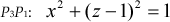
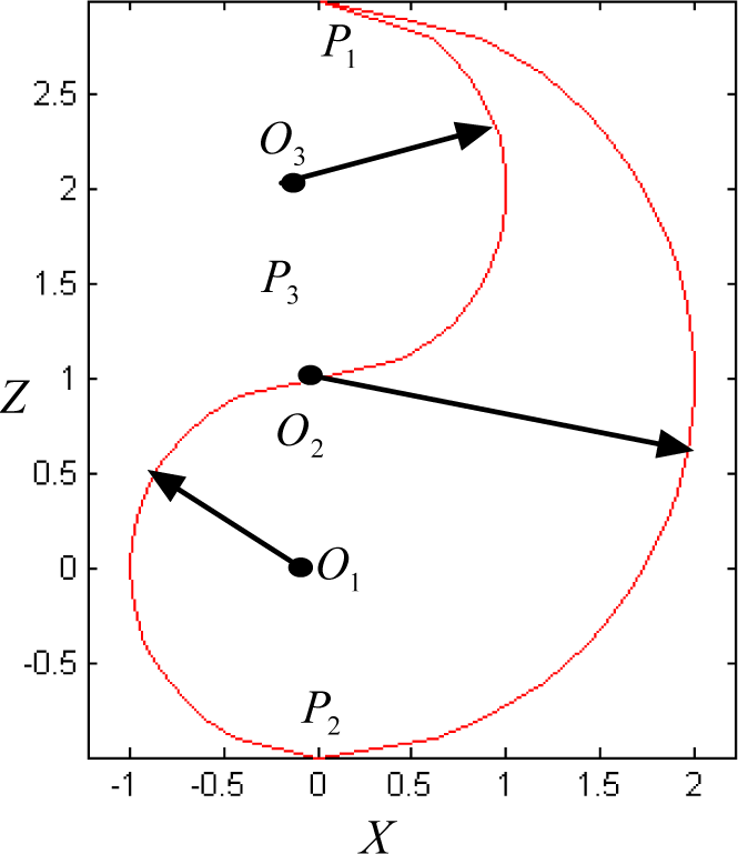
Cross sectional boundary curve of spatial manipulator in XOZ

We can calculate the volume of the workspace by rotating the boundary curve about Z axis in its plan within motion range of θ₁, i.e. solid of revolution. The expression of volume by the numerical integration is:

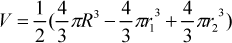
V = \frac{1}{2} (\frac{4}{3} π R^{3} - \frac{4}{3} π r_{1}^{3} + \frac{4}{3} π r_{2}^{3})

(18)

where the R, r₁ and r₂ are the radiuses of arcs P₁P₂, P₂P₃ and P₃P₁. Substituting the radiuses into the equation, the actual size is 16.755.

We adopt Equation (10) again to calculate the percent error of volume

E_{v} = \frac{V_{c} - V_{T}}{V_{T}} \times 100 %

(19)

where the V_c is experiment value resulting from our algorithm, the V_T is the theoretical value 16.755.

Table 2.

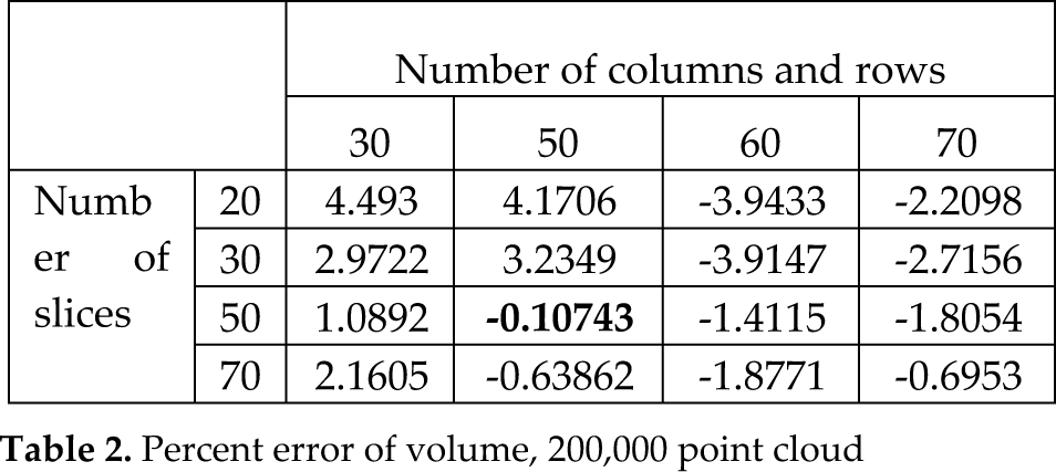
Percent error of volume, 200,000 point cloud

		Number of columns and rows
		30	50	60	70
Number of slices	20	4.493	4.1706	−3.9433	−2.2098
	30	2.9722	3.2349	−3.9147	−2.7156
	50	1.0892	-0.10743	−1.4115	−1.8054
	70	2.1605	−0.63862	−1.8771	−0.6953

Table 3.

Percent error of volume, 300,000 point cloud

		Number of columns and rows
		30	50	60	70
Number of slices	20	4.2274	4.0812	3.9469	−2.5172
	30	3.2259	2.8021	−2.6141	−2.4799
	50	0.46852	−1.2086	−0.9251	−1.4652
	70	1.9636	−1.513	−1.2444	−0.99373

In Table 2 and Table 3, we list the percent error E_v in different partitioned (row and) column number and slice number with Monte Carlo points equals 200,000 and 300,000, respectively. Each value in the tables is the average after 5 calculations.

From Table 2, the minimum error is 0.10743 within 50 columns (rows) and 50 slices, while the minimum error is 0.46852 within 40 columns (rows) and 40 slices for the Table 3. The growth of the number of point cloud improves the accuracy to some extent, but is not significant. According the experiments and trade-off between computing speed and accuracy, the optimal ranges of each parameter for estimating workspace volume are listed below:

Number of point cloud=[200,000, 500,000];

Number of slices=[30, 50];

Number of columns and rows=[40, 70];

where the left value is the minimum, the right is the maximum in the square brackets.

7. Result and discussion

Generally speaking, as the sampling density increases, the output result S' is more likely topologically correct and converges to the original surface S. A good sample should be dense in detailed area and sparse in featureless parts. Usually if the density of point cloud in workspace does not satisfy certain properties required by the algorithm (like good distribution and density, little noise), the depicting program produces incorrect or maybe impossible results. The most important advantage of the Beta distribution is that it can take on many different shapes by changing the parameters. This characteristic provides us a simple way to get more accurate boundary points only by adjust two parameters. It should be pointed out that we still adopt the uniform distribution for the prismatic joint.

Computation time for generating a workspace is an important index to weigh whether a method is practical. Therefore, we measured the computation time in Matlab 7.0 on generating 2D and 3D workspace. For the planar workspace of the 3R manipulator, the elapsed times are 0.375 second (with 10,000 point cloud and 30 sliced columns), 1.047s (with 30,000 point cloud and 50 sliced columns), 2.422s (with 50,000 point cloud and 60 sliced columns), and 5.688s (with 100,000 point cloud and 70 sliced columns). Evidently, the more point cloud, the longer elapsed time. For the 3D workspace of the 3R spatial manipulator, the elapsed times are 21.65s (with 20 slices, 30 sliced columns and rows), 15.422s (with 50 sliced, 50 sliced columns and rows), and 13.266s (with 70 sliced, 70 sliced columns and rows), and the number of point cloud is 200,000 for all the above cases. If the number of point cloud is 300,000, the elapsed times are 40.406s (with 20 slices, 30 sliced columns and rows), 24.016s (with 50 sliced, 50 sliced columns and rows), and 23.687s (with 70 sliced, 70 sliced columns and rows). Supposed the number of point cloud is determined, it is interesting for computing the 3D workspace that with the increase of slices, rows and columns, the elapsed time gradually decreases. This is because the less number of slices the more points exist in each slice, what result to the program needs more time to search boundary points form a large of point cloud within each slice. It should be pointed out, the main configuration of the computer is Core 2 Duo E7300, 2GB RAM, 500GB disk, and the OS is Windows XP. The results showed that the method can satisfy the fast computation from the engineering viewpoints.

In [41], the 3D shape and volume of robot workspace are generated by two softwares. In the near future, we want to construct the 3D shape in one software by 3D reconstruction.

Reconstruction problems occur in diverse scientific and engineering application domains [46-50]. Surface reconstruction can be stated as follows: given a set of sample points Ω assumed to lie on or near an unknown surface S, create a surface model S′ approximating S [50]. The reconstruction methods may be organized as follows:

(1) Surface reconstruction using planar cross sections. To reconstruct the 3D surface of workspace, the relationship of envelope curves in various slices should be given. After we had obtained the 2D curves of different slices, there are both important sub-problems challenging us: contour correspondence and contour titling.

(2) Reconstruction from scattered points obtained from the surface of the object. This type of reconstruction makes no assumption about object topology thus points could be freely acquired. But we have to choose a proper method to create a regular and continuous (triangular) mesh representation from the boundary point cloud.

In the future work, we will address the 3D surface reconstruction from point cloud and/or planar cross sections.

8. Conclusion

A systematic algorithm was developed in this paper to determine and display 2D and 3D manipulators workspace boundary curves and estimate their sizes. This method takes advantage of the properties of the Beta distribution of joint variable and kinematics function to obtain the more accurate approximate workspace composed of point cloud. The area of planar robot manipulator is estimated by regarding the workspace boundary as a polygon. Finally, the volume of workspace is calculated by integrating trapezoidal-based numerical integration and polygon area of each slice.

The algorithm presented here is the primitive result, and works well for most manipulators, especially hyper-redundant robot. In future, the kinematic synthesis of manipulators based on the algorithm will be discussed.

Footnotes

9. Acknowledgments

Project supported in part by the Innovation Scientists and Technicians Troop Construction Projects of Henan Province (No.114100510015), by the National Nature Science Foundation of China (No. 61075183), by the National Key Technology R & D Program of China (No. 2008BADA8B04), by the Young Backbone Teachers Supporting Plan of Henan Province (No.2009GGJS-58), and by the R & D Program of Zhengzhou (No. 083SGYG25121-1)

References

Litvin

F.L.

, “Application of theorem of implicit function system existence for analysis and synthesis of linkages”, Mechanism and Machine Theory, vol.15, no.2, pp .115–125, 1980.

Kohli

Spanos

, “Workspace analysis of mechanical manipulators using polynomial discriminants”, ASME Journal of Mechanisms, Transmissions, and Automation in Design, vol.107 pp.209–215, 1985.

Spanos

Kohli

, “Workspace analysis of regional structures of manipulators”, ASME Journal of Mechanisms, Transmissions, and Automation in Design, vol.107, pp.216–222, 1985.

Haug

E.J.

Wang

J.Y.

J.K.

, “Dextrous workspaces of manipulators I. analytical criteria”, Mechanics of Structures and Machines, vol.20, no.3, pp. 321–361, 1992.

Haug

E.J.

Luh

C.-M.

Adkins

F.A.

Wang

J.-Y.

, “Numerical algorithms for mapping boundaries of manipulator workspaces”, ASME Journal of Mechanical Design, vol.118, pp. 228–234, 1996.

Abdel-Malek

Adkins

Yeh

H.-J.

Haug

, “On the determination of boundaries to manipulator workspaces”, Robotics and Computer-Integrated Manufacturing, vol.13, no.1, pp. 63–72, 1997.

Abdel-Malek

Yeh

H.-J.

Othman

, “Interior and exterior boundaries to the workspace of mechanical manipulators”, Robotics and Computer Integrated Manufacturing, vol.16, pp. 365–376, 2000.

Abdel-Malek

Yang

, “Workspace boundaries of serial manipulators using manifold stratification”, International Journal of Advanced Manufacturing Technology, vol.28, pp. 1211–1229, 2006.

Bergamaschi

P.R.

Nogueira

A.C.

de Fátima Pereira

Saramago , “Design and optimization of 3R manipulators using the workspace features”, Applied Mathematics and Computation, vol.172, no.1, pp. 439–463, 2006.

10.

Yang

Abdel-Malek

Zhang

, “On the workspace boundary determination of serial manipulators with non-unilateral constraints”, Robotics and Computer Integrated Manufacturing, vol. 24, no.1, pp. 60–76, 2008.

11.

Wang

J.Y.

J.K.

, “Dextrous workspaces of manipulators, Part II: Computational methods”, Mechanics of Structures and Machines, vol.21, no.4, pp. 471–506, 1993.

12.

Qiu

C.C.

Luh

C.-M.

Haug

E.J.

, “Dextrous workspaces of manipulators, Part III: Calculation of continuation curvesat bifurcation points”, Mechanics of Structures and Machines, vol.23, no.1, pp. 115–130, 1995.

13.

Luh

C.-M.

Adkins

F.A.

Haug

E.J.

Qiu

C.C.

, “Working capability analysis of Stewart platforms”, ASME Journal of Mechanical Design, vol.118, pp. 220–227, 1996.

14.

Kumar

Waldron

K.J.

, “The workspaces of a mechanical manipulator”, ASME Journal of Mechanical Design, vol.103, pp. 665–672, 1981.

15.

Sugimoto

Duffy

, “Determination of extreme distances of a robot hand- part 1 a general theory”, ASME Journal of Mechanical Design, vol.103, pp. 631–636, 1981.

16.

Sugimoto

Duffy

, “Determination of extreme distances of a robot hand. Part 2: Robot arms with special geometry”, ASME Journal of Mechanical Design, vol.103, pp. 776–783, 1981.

17.

Freudenstein

Primrose

E.J.F.

, “On the analysis and synthesis of the workspace of a three-link, turning-pair connected robot arm”, ASME Journal of Mechanisms, Transmissions, and Automation in Design, vol.106, pp. 365–370, 1984.

18.

Cwiakala

Lee

T.W.

, “Generation and evaluation of a manipulator workspace based on optimum path search”, ASME Journal of Mechanisms, Transmissions, and Automation in Design, vol.107, pp. 245–255, 1985.

19.

Snyman

J. A.

Plessis

, “An optimization Approach to the Determination of the Boundaries of Manipulator Workspaces”, ASME Journal of Mechanical Design, vol.122, pp.447–456, 2000.

20.

Castelli

Ottaviano

Ceccarelli

, “A fairly general algorithm to evaluate workspace characteristics of serial and parallel manipulators”, Mechanics Based Design of Structures and Machines, vol.36, pp. 14–33, 2008.

21.

Vafa

Dubowsky

, “The kinematics and dynamics of space manipulators: The virtual manipulator approach”, International Journal of Robotics Research, vol.9, no.4, pp. 3–21, 1990

22.

Chirikjian

Ebert-Uphoff

, “Numerical convolution on the euclidean group with applications to workspace generation”, IEEE Transactions on Robotics and Automation, vol. 4, no.1, pp.123–136. 1998

23.

Wang

Chirikjian

, “Workspace generation of hyper-redundant manipulators as a diffusion process on se(n)”, IEEE Transactions on Robotics and Automation, vol.20, no.3, pp. 399–408, 2004.

24.

Gupta

K.C.

Roth

, “Design considerations for manipulator workspace”, ASME Journal of Mechanical Design, vol.104, pp. 704–711, 1982.

25.

Lee

T.W.

Yang

D.C.H.

, “On the evaluation of manipulator workspace”, ASME Journal of Mechanisms, Transmissions, and Automation in Design, vol.105, pp. 70–77, 1983.

26.

Selfridge

R.G.

, “The reachable workarea of a manipulator”, Mechanism and Machine Theory, vol.18, no. 2, pp. 131–137 1983.

27.

Tsai

Y.C.

Soni

A.H.

, “An algorithm for the workspace of a general n-R robot”, ASME Journal of Mechanisms, Transmissions, and Automation in Design, vol.105, pp. 52–57, 1983.

28.

Yang

D.C.H.

Lee

T.W.

, “On the workspace of mechanical manipulators”, ASME Journal of Mechanisms, Transmissions, and Automation in Design, vol.105, pp. 62–69, 1983.

29.

Cimino

W.W.

Pennock

G.R.

, “Workspace of a six-revolute decoupled robot manipulator”, In Proceedings of the IEEE International Conference on Robotics and Automation, vol. 3, pp. 1848–1852, San Francisco, California. 1986.

30.

Ceccarelli

, “A formulation for the workspace boundary of general N-revolute manipulators”, Mechanism and Machine Theory, vol.31, no.5, pp. 637–646, 1996.

31.

Ottaviano

Husty

Ceccarelli

, “Identification of the workspace boundary of a general 3-R manipulator”, ASME Journal of Mechanical Design, vol.128, pp. 236–242, 2006.

32.

Sen

Singh

B.N.

, “A geometric approach for determining inner and exterior boundaries of workspaces of planar manipulators”, ASME Journal of Mechanical Design, vol.130, no.2, pp.1–9, 2008.

33.

Alciatore

D. C.

, “Determining manipulator workspace boundaries using the Monte Carlo method and least squares segmentation”. In Proceedings of ASME Robotics: Kinematics, Dynamics and Controls, 1994.

34.

Rastegar

Perel

, “Generation of manipulator workspace boundary geometry using the Monte Carlo method and interactive computer graphics”, ASME Journal of Mechanical Design, vol. 112, pp. 452–454, 1990.

35.

Rastegar

Fardanesh

, “Manipulation workspace analysis using the Monte Carlo Method”, Mechanism and Machine Theory, vol.25, no.2, pp.233–239, 1990.

36.

Guan

Yokoi

, “Reachable space generation of a humanoid robot using the Monte Carlo method,” in Proceedings of IEEE/RSJ International Conference Intelligent Robots and Systems, October; Beijing, China, pp.1984–1989, 2006.

37.

Guan

Yokoi

Zhang

, “Numerical methods for reachable space generation of humanoid robots”, The International Journal of Robotics Research, vol.27, no. 8, pp. 935–950, 2008

38.

Cao

S.P.

Zang

Yang

G.Y.

, “Shape and size computation of planar robot workspace”, in Proceedings of WRI World Congress on Computer Science and Information Engineering, Vol.2, Los Angeles, USA. pp.126–130, March, 2009

39.

Cao

“An improved method for depicting workspace boundary of planar robot manipulator”, in Proceedings of International Joint Conference on Computational Sciences and Optimization, vol. 1, pp. 77–78, 2010

40.

Cao

S.P.

Zang

Yang

G.Y.

, “An integrated method for workspace computation of robot manipulator”, in Proceedings of International Joint Conference on Computational Sciences and Optimization, vol. 1, pp. 309–312, Sanya, China. April, 2009.

41.

Cao

Zang

, “An engineering-oriented method for the three dimensional workspace generation of robot manipulator” Journal of Information and Computational Science, Vol. 8, no.1, pp. 51–61, 2011

42.

Richard

P. Paul

, “Robot manipulators: Mathematics, programming, and control: The computer control of robot manipulators”. MIT Press, Cambridge, Mass, 1981

43.

Bain

Lee J.

Max

Engelhardt

. “Introduction to probability and mathematical statistics”, Wadsworth Publishing Company, November, 1991.

44.

Beyer

W. H.

(Ed.). “CRC Standard Mathematical Tables”, 28th ed. Boca Raton, FL: CRC Press, 1987.

45.

Mathews

J. H.

Fink

K. D.

, “Numerical Methods Using MATLAB,” 3rd ed. New Jersey:Prentice Hall, 1999.

46.

Soroka

B. I.

, “Generalised cones from serial sections”, Computer Vision Graphics and image Processing, vol. 15, pp. 154–166, 1981.

47.

Haig

T. D.

Attikiouzel

Alder

, “Border marriage: Matching of contours of serial sections”, IEEE Proceedings of Communications, Speech and Vision, vol.138, no. 5, pp371–376, 1991

48.

Owada

Shinagawa

Nielsen

, “Enumeration of contour correspondence,” International Journal of Image and Graphics, vol.3, no. 4, pp. 609–628, 2003

49.

Skinner

S.M.

, “The correspondence problem: Reconstruction of objects from contours in parallel sections”, Master's thesis, University of Washington, Washington D.C., 1991.

50.

Chui

C. K.

, “An introduction to wavelets”, Boston: Academic Press, Inc., 1992.

51.

Pratt

“Direct least-squares fitting of algebraic surfaces”, Computer Graphics, vol. 21, pp. 145–152, 1987

Accurate Numerical Methods for Computing 2D and 3D Robot Workspace

Abstract

Keywords

1. Introduction

2. Two illustrative examples

3. Features of the previous method

4. A Beta-distribution based method

4.1. Distribution characteristics of Monte Carlo points in workspace

4.2. Probability density distribution of manipulator joints variables

4.3. Beta Distribution and determination of parameters

5. Area computation of robot workspace based on polygon

5.1. Algorithm description

5.2. Error comparison

6. Boundary curves of 3D robot manipulator and volume calculation

6.1. Depicting boundary curves of 3D robot manipulator

6.2. Volume calculation

7. Result and discussion

8. Conclusion

Footnotes

9. Acknowledgments

References