Sage Journals: Discover world-class research

Abstract

Global localization problem is one of the classical and important problems in mobile robot. In this paper, we present an approach to solve robot global localization in indoor environments with grid map. It combines Hough Scan Matching (HSM) and grid localization method to get the initial knowledge of robot's pose quickly. For pose tracking, a scan matching technique called Iterative Closest Point (ICP) is used to amend the robot motion model, this can drastically decreases the uncertainty about the robot's pose in prediction step. Then accurate proposal distribution taking into account recent observation is introduced into particle filters to recover the best estimate of robot trajectories, which seriously reduces number of particles for pose tracking. The proposed approach can globally localize mobile robot fast and accurately. Experiment results carried out with robot data in indoor environments demonstrates the effectiveness of the proposed approach.

Keywords

robot localization global localization scan matching pose tracking particle filters

1. Introduction

The problem of localization has attracted immense attention in the robotic literatures. It addresses the problem of estimating the robot pose (position and orientation) relative to a given map with onboard sensors. In fact, the localization problem is to compensate for sensor noise and odometer reading errors (Milstein, A. et al., 2002). And two different cases can be distinguished (Thrun, S. et al., 2005): given the initial knowledge of robot's pose, the localization problem is a pose tracking problem; with unknown initial pose, the localization problem turns to be global localization problem. Hence, global localization subsums the pose tracking problem.

In robotic literature, there are mainly three kinds of approaches providing a solution to global localization problem: Extented Kalman Filter (EKF) algorithms (Thrun, S. et al., 2005),Grid localization and Monte Carlo localization (MCL) algorithms (Dellaert, F. et al.,1999). EKF are computationally efficient and can deal with slight non-linear systems, but become sub-optimal when the dynamic models are serious non-linearity. What's more, it assumes that the control and measurement noises are Gaussian. Grid localization method seems more robust to non-linearity and arbitrary noise distributions, but it ignores the computational complexity problem, when applied to large scale environments. To overcome these limitations, MCL was introduced as an effective solution to solve pose tracking (Dellaert, F. et al., 1999; Thrun, S. et al., 2005). In statistical literature, Monte Carlo method is known as particle filter, so we call it particle filter in this paper.

Over the last years, particle filters have been applied with great success in mobile robot, including mobile robot localization (Thrun, S. et al., 2001; Fox, D., 2003), map building (Doucet, A., 2000) and fault detection (Freitas, N., 2002). The main problem of particle filter approach is their complexity, measured in terms of the number of required particles. Therefore, reducing this quantity is one of the major challenges of this family of algorithms (Grisetti, G., 2007).

Since there is no initial knowledge of robot pose in global localization, the particle filter based localization algorithms need very large number of particles to localize robot. Although the KLD-sampling strategy (Fox, D., 2003) is proposed to adapt the number of particles during localization, there are not very quickly converge to a single likelihood pose. And this strategy is not very functionary during pose tracking stage, because the uncertainty does not vary much in this stage, so the variety of particle number is small (Blanco, J.L. et al., 2008). But the the calculation of KL-distance at each step increases the computational complexity.

This paper proposes a new approach to solve the global localization problem in indoor environments represented by grid maps. Different from previous approaches, we divide global localization problem into two separate stages : get the initial pose of robot and track the robot poses. During the first stage, one laser scan data can be used to get the initial pose in short time; then particle filter is employed to estimate the robot trajectories with a sample-based representation. To reduce the number of particles, a scan matching technique called Iterative Closest Point (ICP) (Besl P., 1992;) is used to amend the robot motion model, it can drastically decreases the uncertainty about the robot's pose in prediction step. Then accurate proposal distribution taking into account recent observation is introduced into particle filters to recover the best estimate of robot trajectories, which seriously reduces number of particles for pose tracking.

The rest of this paper is organized as follows. After explaining how a particle filter can be used in general to solve the pose tracking problem, we present our approach in Section III. We then provide implementation details in Section VI. Experiment results carried on real robots data set are presented in Section VI. The last section concludes with some discussions.

2. Robot localization with particle filters

Suppose the initial knowledge of robot pose p(x₀) is provided by some appropriate methods. Then the global localization turns to be the pose tracking problem. The key idea of particle filter for pose tracking is to estimate the robot trajectories with a sample-based representation. Given odometry reading u_1:t = {u₁,u₂,…,u_t} and sensor observations z_1:t = {z₁, z₂,…,z_t}, the primary goal is to recover the best estimate of robot trajectories:

p (x_{1 : t} | z_{1 : t}, u_{1 : t})

(1)

Based on the Bayes' rule, it can derive a recursive filter to update the trajectory x^[i]_1:t samples during each iteration. And each iteration process can be summarized by the following steps:

(1).

Sampling : With the the previous generation {x^[i]_1:t-1}, draw (sample) the next generation of particles {x^[i]_1:t} from the proposal distribution π(η). The selection of proposal distribution can greatly influence the performance of algorithm itself.

(2).

Importance weighting: Calculated an importance weight for each particle:

\begin{array}{l} w_{t}^{[i]} = \frac{p (x_{1 : t}^{[i]} | z_{1 : t}, u_{1 : t}, m)}{π (x_{1 : t}^{[i]} | z_{1 : t}, u_{1 : t}, m)} \\ \propto w_{t - 1}^{[i]} \frac{p (z_{t} | x_{t}^{[i]}, m) p (x_{t}^{[i]} | x_{t - 1}^{[i]}, u_{t})}{π (x_{t} | x_{1 : t - 1}^{[i]}, u_{1 : t}, z_{1 : t}, m)} \end{array}

(2)

Most of the existing particle filter application reply on this recursive structure.

(3).

Resampling : Particles are drawn with replacement proportional to their importance weight, which means a particle with small weight maybe replaced by a particle with large weight.

Often, a probabilistic odometry motion model is used as the proposal distribution in the simultaneous localization and mapping (SLAM) or localization algorithm. But the odometry readings are always noisy and there needs large number of particles to avoid filter divergence. In following section, we will describe a technique that can get the initial pose with only one laser scan and compute a more accurate proposal distribution.

3. Effective global localization algorithm

In this section, we first analyze the property of indoor environments and present an efficient approach to acquire the initial pose of robot with only one laser scan. Given the initial knowledge of robot's pose, we use a particle filter with accurate proposal distribution to track robot pose in real time.

3.1 Initial pose acquiring

In 2D plane, the robot pose is composed of robot position (t_x, t_y) and orientation θ. A simple method that can acquire the initial pose of robot is to using a grid sampling representation of the pose configuration space (Lina, M. P., 2006; Thrun, S. et al., 2005). As shown in Fig. 1, each grid cell represents a robot pose in the environment and different planes represent different robot orientations. Then the observation can be used to calculate the probability values of each grid and the grid with the largest weight is selected as the robot pose. Since the robot pose has three dimensions in plane, the number of grid cells is cubic. Hence, more efficient approach is necessary.

Figure 1.

Grid sampling representation of the pose configuration space

Before introducing the initial pose acquiring, we can analyze the characteristics of laser scan data and grid map. A laser scan data is some two dimensional points in Cartesian coordinate, with the center of laser range finder as its coordinate origin. And the grid a pis composed of many cells, with the state stored in the matrix. It is difficult to directly deal with two different kinds of data. Compared to one laser scan, a grid map contains much more information. Under the premise of ensuring accuracy, we can only select the cells of grid map with occupied state and view them as points with defined Coordinate value. That's means the problem of initial pose acquiring in gird map can also be viewed as scan matching problem between point set. In most engineered indoor environments, major structures, such as doors, walls, cupboards, etc., can be represented by sets of lines in 2D plane. Hence, Hough Scan Matching (HSM) (Censi, A. et al., 2005) can be used to estimate the orientation of robot θ.

In the 2D plan, a line can be easily parameterized as a collection of points (x, y) as follows:

x \cos φ + y \sin φ = r

(3)

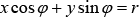
where φ ∈ [0, 2π) and r ⩾ 0. Suppose the pose of robot in gird map is (t_x, t_y, θ). After transformation, the laser scan points (x_q, y_q) become the point in grid map:

{\begin{matrix} x = \cos θ x_{q} - \sin θ y_{q} + t_{x} \\ y = \sin θ x_{q} + \cos θ y_{q} + t_{y} \end{matrix}

(4)

By introducing the Eq. (4) into Eq. (3), we can get Eq. (5):

x_{q} \cos (φ - θ) + y_{q} \sin (φ - θ) = r + [\cos φ \sin φ] t

(5)

Given the quantization precision of the parameter pairs (θ, r), we can build two Hough tables [15]. Take each point and vote for all lines that could go through it, we can get two Discrete Hough Transforms (DHT) with following relation:

{DHT}_{Q} (φ - θ, r + [\cos φ \sin φ] t) = {DHT}_{P} (φ, r)

(6)

With the definition of Hough Spectrum presented in (Censi, A. et al., 2005), we can get two Discrete Hough Spectrum: DHS_P(φ) and DHS_Q(φ-θ). As the HSM, we can get the estimation of robot orientation by the correlations of the two spectra:

corr (θ) = \sum_{φ \in [0, 2 π)} DH S_{P} (φ) DH S_{Q} (φ - θ)

(7)

Where θ ∈ (−π, π]. If there are no symmetrical or alike structures in indoor environments, the global maximum of the correlation is much larger than other local maxima and the global maximum can be view as the solution of robot orientation. Hence, the pose configuration space now descends into a plane (such as the yellow plane shown in Fig. 1). Then we only need to get the position of the robot in a plane.

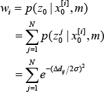
Combined with the orientation, each grid in the plane represents a possible robot pose. Suppose the robot pose in gird map is x^[i]]₀, we can compute the likelihood of the laser scan by “beam endpoint model” [3]: for one laser beam, there is a cell with occupied state in grid map that has the nearest Euclidean distance to the end of this laser beam. If the nearest Euclidean distance from the beam end to cell is Δd_ij, then likelihood of the laser scan for one pose x₀^[i] is:

\begin{array}{l} w_{i} = p (z_{0} | x_{0}^{[i]}, m) \\ = \sum_{j = 1}^{N} p (z_{0}^{j} | x_{0}^{[i]}, m) \\ = \sum_{j = 1}^{N} e^{- {(Δ d_{i j} / 2 σ)}^{2}} \end{array}

(8)

After calculating weight for all possible pose, pose with largest weight can be selected as the initial robot pose.

In order to eliminate the quantization errors, gradient descent search algorithm can be employed to get more accurate initial robot pose.

3.2 Pose tracking

For pose tracking, a particle filter is used. The original particle filter based algorithm was proposed by Dellaert (Dellaert, F. et al., 1999). Based on the pose tracking results of previous generation, the next generation of particles is sampled for a probability odometry motion model, and an individual importance weight is assigned to each particle, according to suboptimal observation model (Grisetti, G et al., 2007). Since the odometer reading is noisy and the proposal distribution only uses the odometer reading, it need high number of particles to track robot pose. To overcome this problem, one can improve the robot motion model and consider the most recent sensor observation when generating the next generation of samples.

3.2.1 Improved motion model

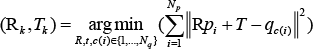
In this section, we will introduce how to use Iterative Closest Point (ICP) (Besl & McKay, 1992) algorithm to improved the motion model. ICP algorithm is a popular algorithm in robotics, which can assign correspondences between two sets of points and recover the transformation that maps one points set to the other. It is simple and has computational complexity, while it has accurate results. Since the information of laser range finder (usually, with a SICK Laser Measurement Sensor (LMS)) equipped on robot is significantly more precise than the motion estimate of robot based on the odometry. It is reasonable to estimate motion of robot by using ICP with two adjacent laser scans, which are mostly overlap. Suppose the laser scan points at time (t-1) are Q = {q_i}^{N
_q}_i=1 and at time t are P = {p_i}^{N
_p}_i=1. The relative transformations of robot pose between time (t − 1) and t can be calculated as:

\begin{array}{l} \min_{R, T, c (i) \in {1, ..., N_{q}}} (\sum_{i = 1}^{N} {‖ R p_{i} + T - q_{c (i)} ‖}^{2}) \\ s . t . R^{'} R = I \det (R) = 1 \end{array}

(9)

where q_c(i) is the closest point for p_i, R is a rotation matrix and T is a translation vector. ICP algorithm solves the least square problem presented in Eq. (9) by using two iterative steps:

(1).

With the transformation results get in previous iteration k, construct the new correspondence for each point in data sets P from data set Q:

c (i) = \underset{j \in {1, ..., N_{q}}}{\arg \min} ({‖ R_{k - 1} p_{i} + T_{k - 1} - q_{j} ‖}^{2})

(10)

(2).

Based on the new correspondence set, calculate new transformation as follows:

(R_{k}, T_{k}) = \underset{R, t, c (i) \in {1, ..., N_{q}}}{\arg \min} (\sum_{i = 1}^{N_{p}} {‖ R p_{i} + T - q_{c (i)} ‖}^{2})

(11)

Eq. (10) can be solved by many efficient methods, such as the nearest point search based on k-d tree algorithm or its variants (Greenspan & Yurick, 2003; Nuchter et al., 2007) and Eq. (11) can be solved by many methods (Nuchter et al., 2010). For 2D scan matching problem, an efficient solution is presented in (Lu & Mlios, 1997). When ICP algorithm is convergent, we can recover the relative transformation ŝ_t of robot pose between time (t − 1) and t (Lu F. & Mlios E., 1997). Because ICP performs explicit point-to-point data association during iteration, which can introduces error since the points in each scan represent a surface and not a set of discrete locations. For simplify, we assume the error distribution of ICP results is Gaussian, with zero means and constant variance ∑.

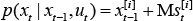
Finally, the motion estimate of robot p(x_t | x_t-1, u_t) can be calculated by using ICP results:

p (x_{t} | x_{t - 1}, u_{t}) = x_{t - 1}^{[i]} + M s_{t}^{[i]}

(12)

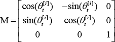
Where s_t^[i] ~ N(ŝ_t, ∑_t), and M is a matrix defined as:

M = [\begin{matrix} \cos (θ_{t}^{[i]}) & - \sin (θ_{t}^{[i]}) & 0 \\ \sin (θ_{t}^{[i]}) & \cos (θ_{t}^{[i]}) & 0 \\ 0 & 0 & 1 \end{matrix}]

Because the ICP results are very accurate, so we can use it to replace odometry readings and get a very accurate motion estimate of robot.

3.2.2 Accurate proposal distribution

Previous pose tracking algorithm use the odometery motion model p(x_t | x_t-1, u_t-1) as the proposal distribution (Dellaert, F. et al., 1999; Fox, D., 2003). Although it is easy to compute for most types of robot, it has high risk of filter divergence. In this paper, we use the more informed proposal p(x_t | x_t-1, u_t, z_t, m), which take into account recent observation z_t. According to Bayes' rule, the distribution:

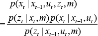
\begin{array}{l} p (x_{t} | x_{t - 1}, u_{t}, z_{t}, m) \\ = \frac{p (z_{t} | x_{t}, m) p (x_{t} | x_{t - 1}, u_{t})}{p (z_{t} | x_{t - 1}, u_{t}, m)} \end{array}

(13)

By introducing the Eq. (13) into Eq. (1), we can get

\begin{array}{l} w_{t}^{[i]} \propto w_{t - 1}^{[i]} p (z_{t} | x_{t - 1}^{[i]}, u_{t}, m) \\ = w_{t - 1}^{[i]} \int p (z_{t} | x^{'}, m) p (x^{'} | x_{t - 1}^{[i]}, m) d x^{'} \end{array}

(14)

When modeling the environment with a grid map, there are two kinds of approximation of this informed proposal.

Suppose, N particles are used to track robot pose. They first one approximates the sensor model with a Gaussian (Grisetti, G. et al., 2007) model and the second one approximate it by sampling M localization samples for each particles, then resample N particles from the whole N x M samples at resampling step (Grzonka, S. et al., 2009) . Here, we adopt the second one.

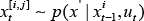
For each particles, draw M samples according to motion model:

x_{t}^{[i, j]} \sim p (x^{'} | x_{t - 1}^{i}, u_{t})

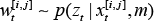
And it's corresponding weight is calculated as follows:

w_{t}^{[i, j]} \sim p (z_{t} | x_{t}^{[i, j]}, m)

(15)

The samples for each particle can approximate term inside the integral in Eq. (14). We can draw N new particles x_t^[i] from the whole samples set according to their importance weights w_t^[i,j]. And each new particle has the same importance weights. The whole robot pose process can be described as shown in Fig. 2. In order to weight each samples, it needs to calculate the observation likelihood p(z_t | x,m). Here, we use the method called “beam end model” as Eq. (8).

Figure 2.

The whole process of robot pose tracking. The red histograms visualize the current weight of each samples.

According to motion model, draw M localization samples for each particles and use the recent observation to weight each sample, resample N particles from the whole N x M samples.

3.3. Global localization algorithm

Hence, from what is discussed above, the overall global localization process can be described as follows:

(1).

Using the first measurement (u₀, z₀) to get the initial robot pose in grid map.

(2).

With ICP, calculate the relative transformation of robot pose between two consecutive time step and get the accurate motion estimate of robot p(x_t | x_t-1, u_t).

(3).

For each pose tracking particle, draw M samples from p(x_t | x_t-1, u_t).

(4).

Calculate the weight p(z_t | x, m) for each sample by using “beam end model”.

(5).

Resampling N particles from the whole sample set, which has N x M samples.

(6).

If there is new measurement arrived, return to step (2).

Implement the above steps until these is no new observation.

4. Experimental Results

In this Section, we outline the experimental results and some analysis. To demonstrate the good performance of the proposed algorithm, it was tested on an opened data set collected by a robot, which is equipped with a LMS. And the data set is collected in indoor environment (Eliazar, A. & Parr, R., 2002). The gird map of the indoor environment is depicted in Fig. 3. All experiments are tested on a PC with 3.0 GHz Dual-Core. Since the ground truth of robot trajectory is not available, a fixed number of 100,000 particles are used to estimate the approximate trajectory.

Figure 3.

Grid Map used for localization. The red trajectory is the path followed by robot during data collection. The points A and B mark the start and end point for the global localization experiments respectively.

4.1. Initial Pose acquiring

Before tracking robot pose, it is necessary to acquiring the initial knowledge of robot's pose. One simple method is to use the raw grid sampling method presented in (Paz, L. M., 2005) to estimate initial robot pose. Since the pose has three dimensions, the number of grid is cubic and the real-time performance is poor. However, we can firstly estimate the robot orientation by using HSM. As shown in Fig.4, the global maximum value of the correlation results is large than other three local maxima, hence it can be selected as robot's orientation. This process only costs 76 ms. As shown in Fig.1, the pose configuration space new becomes quadratic. With the voting process employed in (Paz, L. M., 2005), we can get the weight for each position in the grid. And the voting results are depicts in Fig.5. The gird with the largest weight can be selected as the initial position of the robot. Combined with the robot orientation got from HSM, we can get the initial robot pose with some level quantization errors. Suppose the quantization precisions are 0.2m for robot position and 1deg for robot orientation, and the voting process costs 600ms. If we use the raw grid sampling algorithm, it will cost more than 200s to acquire the initial robot pose. In order to eliminate the quantization errors, gradient descent search algorithm can be use to get the fairly accurate results. The search process costs about 16ms. In one word, the proposed method can get the initial robot pose in one second and only with one laser scan data.

Figure 4.

DHS for grid map and the first laser scan, with their correlation results

Figure 5.

The voting results for each robot's position grid. All the weights of each gird are divided by the largest weight along themself.

If there are symmetrical or alike structures in indoor environments, there may be several local maxima closed to the global maximum value in DHS's correlation results. At this time, several ordered local maxima should be kept in order to avoid losing true orientation value. So does it for position acquiring process. If this happens, initial pose acquiring process will costs more time and may be more laser scans are needed to get the true pose. Someone may ask why don't use HSM to get the robot position directly, this is due to the fact that HSM is irresponsible for acquiring translation (robot's position) results when applied to large environments. (Censi, A. et al., 2005).

A typical SICK LMS has only a 180deg field-of-view, with a fixed resolution 1deg (or 0.5deg) and a maximum range of 8.1m. Hence a laser scan data has limit information. When a robot starts at one point in a long corridor, it maybe failed to acquire the initial robot pose. One possible way is to use two LMSs to consist of a scan system with 360° field of view, which can increase the reliability of initial pose acquiring method.

4.2 Pose tracking

Since the initial robot pose is acquired, pose tracking algroithm can be used to estimate the robot trajectory. For readability, the following abbreviations are employed to denote the alternative localization approaches.

PFO: Standard particle filter based pose tracking approach with odometry-based proposal.

PFI: Standard particle filter based pose tracking approach with ICP results to replace the odometry readings.

PFOI : Our pose tracking approach with ICP result and recent observation to calculate the accurate proposal.

Before comparing the precision, we use odometry readings and ICP algorithm to estimate robot pose respectively. As shown in Fig.6, the odometry readings are noisy. After loop closing, the estimated position of robot is far away from the true position. If we use the odometry reading to calculate the proposal distribution, we can only get a suboptimal proposal. As a result, one needs a comparably high number of particles to track the robot pose. However, the laser scan data are significantly precise and reliable. We can use ICP algorithm to estimate the robot transformation between two consecutive time steps. Compared to odometry reading, the robot poses estimated by ICP are more accurate. And the proposal distribution will be more accurate, if the odometry readings are replaced by ICP results. Although the odometer readings are replaced by ICP results, it is essential. In some situations, ICP may be failed. At this time, the odometer readings can be adopted to calculate the proposal.

Figure 6.

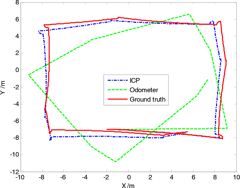
The robot trajectories predicted by ICP and Odometry reading. The red one is the ground truth (approximate) estimated by 100,000 particles.

Because the odometry readings are noisy, the PFO can not get accurate estimated trajectory, even with high number of large particles. Fig.7 depicts the estimate trajectory based on PFO with 500 particles. At the same time, 5 particles are used in PFI and PFOI to estimate robot trajectory and the results are also depicted in Fig.7 and Fig.8 Compared with estimated results of PFO, the proposal calculated from ICP results can get accurate trajectory, even with low number of particles. Since the accurate proposal takes into account the most recent observation, the PFOI can get the most accurate estimated trajectory.

Figure 7.

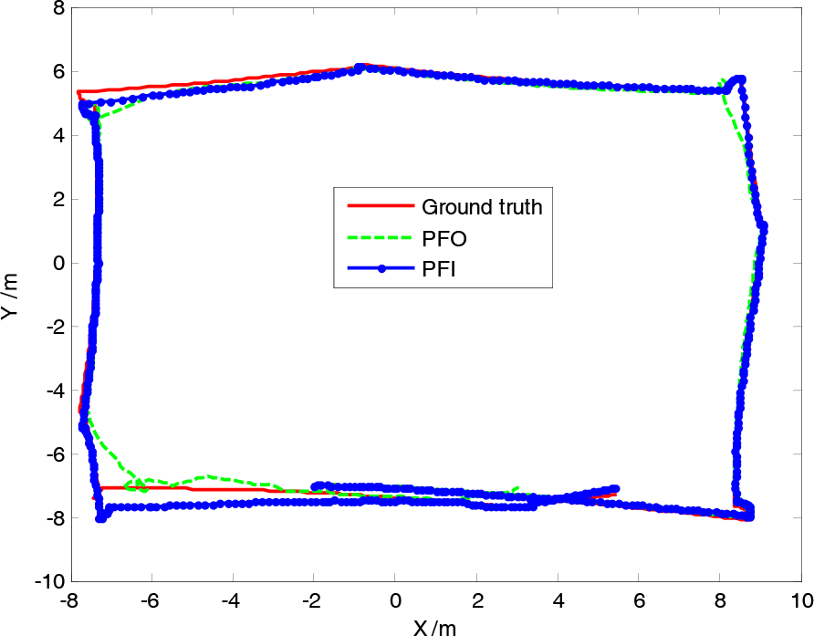
The robot trajectories estimated by two different algorithms. The number of particles used in PFO and PFI are 500 and 5 respectively.

Figure 8.

The robot trajectory estimated by PFOI with only 5 particles. The red one is the ground truth (approximate) and the green one is estimated by PFOI.

To compare PFO and PFOI more deeply, we changed the number of particles for each of them and estimated robot trajectory respectively. As shown in Fig.9, when low number of particles is used, the estimated results of PFOI are more accurate than that of PFO. When the number of particles is over 30, they almost have the same precision. Usually, the LMS can collect 30 scans in 1 second (33ms per scan). If 20 particles are used, the rum time for dealing with each scan is about 20ms in PFOI, which is little than the collected time for each scans. That's mean the proposed approach can localize the robot in grid map in real time.

Figure 9.

Localization error (mean) for different approaches with different number of particles.

5. Conclusions

In this paper, we proposed an improved approach to solve robot global localization in indoor environments. It can acquire the initial knowledge of robot's pose in short time, with only one laser scan data. Then a particle filter can be used to track robot pose. In order to calculate accurate proposal distribution, our approach replaces the noisy odometry readings by ICP results and takes into account the recent observation. When it estimate robot trajectory, the proposed approach employs a fixed number of particles. It has been tested and evaluated on an opened data acquired with a robot equipped with laser range finder scan. To get the same precise localization results, the number of particles needed in the proposed approach is one order of magnitude lower than that of previous approaches. Experiment results show that the proposed approach can accurately localize robot in real time.

Footnotes

6. Acknowledgment

This work is supported by the National Natural Science Foundation of China under Grant No. 90820017, the National Basic Research Program of China under Grant No. 2007CB311005. The authors would like to thank Eliazar, P. and Parr P. for providing the laser data sets.

References

Milstein

Sánchez

J. N.

& Williamson

E. T.

(2002). Robust Global Localization Using Clustered Particle Filtering. Proceedings of the Eighteenth National Conference on Artificial Intelligence, Alberta, Canada, pp. 581–586 Aug. 2002

Thrun

Burgard

& Fox

(2005). Probabilistic Robotics, MIT Press, ISBN 0-262-20162-3, Lodon

Dellaert

Fox

Burgard

Thrun

(1999). Monte Carlo localization for mobile robots. Proceedings of the IEEE International Conference on Robotics and Automation, pp. 1322–1328. IEEE, Michigan

Thrun

Fox

Burgard

& Dellaert

(2001). Robust Monte Carlo Localization for Mobile Robots. Artificial Intelligence, Vol. 128, No. 1–2, pp. 99–141, ISSN : 11076-9757

Fox

(2003). Adapting the sample size in particle filters through KLD-sampling. International Journal of Robotics Research IJRR, Vol. 22, No. 12, pp.985–1003 2003. ISSN: 0278-3649

Doucet

Freitas

Murphy

& Russel

(2000). Rao-Blackwellized particle filtering for dynamic Bayesian networks, Proceedings of the Conference Uncertainty Artif. Intell., pp. 176–183. Stanford, CA, Jul. 2000

Grisetti

Stachniss

& Burgard

(2007). Improved Techniques for Grid Mapping with Rao-Blackwellized Particle Filters, Transactions on Robotics, Vol. 23, No. 1, pp. 34–46, ISSN: 1552-3098.

Freitas

(2002). Rao-Blackwellised particle filtering for fault diagnosis, IEEE Aerospace Conference Proceedings. Vol, 4. pp. 1767–1772, ISBN: 0-7803-7231-X

Lina

M. P.

Piníes

Neira

& Tardós

J.D.

(2005). Global Localization in SLAM in Bilinear Time, Proceedings of IEEE/RSJ Int. Conf. on Intelligent Robots and Systems, pp. 655–661, Edmonton, Canada, Aug. 2005.

10.

Besl

& McKay

(1992). A method for registration of 3-D shapes. IEEE Transactions on Pattern Analysis and Machine Intelligence, Vol. 14, No. 2, pp. 239–256, ISSN: 0162-8828

11.

Blanco

J.L.

Gonzalez

& Fernandez-Madrigal

J.A.

(2008). An Optimal Filtering Algorithm for Non-Parametric Observation Models in Robot Localization. Proceedings of the IEEE International Conference on Robotics and Automation, pp. 461–466. California, May 2008

12.

Censi

Iocchi

& Grisetti

(2005). Scan matching in the Hough domain, Proceedings of the IEEE International Conference on Robotics and Automation, Barcelona, Spain, pp. 2739–2744.

13.

Greenspan

& Yurick

(2003). Approximate k-d tree search for efficient icp, in Proc. 4th Int. Conf. 3D Digital Imaging and Modeling (3DIM), pp. 442–448.

14.

Nuchter

Lingemann

& Hertzberg

. (2007). Cached k-d treesearch for icp algorithms, in Proc. 6th Int. Conf. on 3D Digital Imaging and Modeling(3DIM), pp.419–426.

15.

Nuchter

Elseberg

Schneider

& Paulus

(2010). Study of Parameterizations for the Rigid Body Transformations of The Scan Registration Problem, Journal Computer Vision and Image Understanding, Vol. 114, No. 8, pp. 963–980, ISSN 1077-3142

16.

& Milios

(1997). Robot pose estimation in unknown environments by matching 2D range scans. Journal of Intelligent and Robotics Systems, Nol. 18, No. 3, pp. 249–275, ISSN: 0921-0296

17.

Eliazar

& Parr

(2002). DP-SLAM: Fast, robust simultaneous localization and mapping without predetermined landmarks, Proceedings of Int. Conf. Artif. Intell., pp. 1135–1142, Acapulco, Mexico, March 2003

An Improved Technique for Robot Global Localization in Indoor Environments

Abstract

Keywords

1. Introduction

2. Robot localization with particle filters

3. Effective global localization algorithm

3.1 Initial pose acquiring

3.2 Pose tracking

3.2.1 Improved motion model

3.2.2 Accurate proposal distribution

3.3. Global localization algorithm

4. Experimental Results

4.1. Initial Pose acquiring

4.2 Pose tracking

5. Conclusions

Footnotes

6. Acknowledgment

References