Sage Journals: Discover world-class research

Abstract

Finding optimal trajectory is critical in several applications of robot manipulators. This paper is applied the open-loop optimal control approach for generating the optimal trajectory of the flexible mobile manipulators in point-to-point motion. This method is based on the Pontryagin's minimum principle that by providing a two-point boundary value problem is solved the problem. This problem is known to be complex in particular when combined motion of the base and manipulator, nonholonomic constraint of the base and highly non-linear and complicated dynamic equations as a result of flexible nature of links are taken into account. The study emphasizes on modeling of the complete optimal control problem by remaining all nonlinear state and costate variables as well as control constraints. In this method, designer can compromise between different objectives by considering the proper penalty matrices and it yields to choose the proper trajectory among the various paths. The effectiveness and capability of the proposed approach are demonstrated through simulation studies. Finally, to verify the proposed method, the simulation results obtained from the model are compared with the results of those available in the literature.

Keywords

Elastic mobile robotic arms Optimal motion planning Pontryagin's minimum principle

1. Introduction

Mobile manipulators due to their extended workspace offer an efficient application for wide areas. However, these systems are usually “power on board” with limited capacity. Hence, using light links can minimize the inertia and gravity effects on actuators. This helps the mobile manipulator to work in energy - efficient manner and pilots us to use of flexible manipulators.

The platform path planning was investigated for a given end-effector path with assuming that the robot is redundant (Chen M.W. & Zalzala A.M.S., 1997). Then, the robot configuration was determined by minimizing the overall actuation torque and maximizing the manipulability criterion. By employing an appropriate mapping, Papadopoulos et al. transformed the three differentials of the nonholonomic constraint into two differentials and designed the path via polynomial functions (Papadopoulos E. G. & Poulakakis J., 2001). Tanner by implementing a potential field technique using point-world topology proposed a methodology to motion planning for multiple mobile manipulators cooperation that is applicable to articulated, non point nonholonomic robots with guaranteed convergence properties (Tanner H.G., 2003). Sun et al. discussed the load distribution and joint trajectory planning of two robots with one flexible link (Sun Q., 1999). The control of two-link flexible manipulators was studied on the basis of quasi-static equation (Matsuno F. & Hatayama M., 1999). Subudhi and Morris presented a dynamic modeling technique for a manipulator with multiple flexible links and flexible joints based on a combined Euler–Lagrange formulation and assumed modes method. Then, they controlled such system by formulating a singularly perturbed model and used it to design a reduced-order controller (Subudhi B. & Morris A.S., 2002). Path planning of a flexible manipulator was formulated as a discrete-time open-loop optimal control problem which its solution was done via discrete dynamic programming (Wilson D.G. et al., 2004). The assumed mode expansion method was used to derive the dynamic equation of fixed base flexible manipulator (Green A. & Sasiadek J.Z., 2004).

In above-mentioned works, only base mobility or link flexibility has been considered, and the synthesis of the mobile base with flexible links has not been studied. However, as explained before, the flexible links manipulator mounted on the mobile platform can exhibit many advantages. Such systems require less material, consume less power, require smaller motors and they reduce the torque capacity; hence, they can improve the efficiency of the system noticeably. The maximum payload of flexible mobile manipulator was determined along the given trajectory using finite element approach. So, the study did not consider finding the optimal path (Korayem M.H. et al., 2008). A computational algorithm was presented to determine the maximum payload. In this study, linearizing the dynamic equations and constraints are done on the basis of Iterative Linear Programming (ILP) approach for flexible mobile manipulators (Korayem M.H. & Ghariblu H., 2004). But, in ILP method, final boundary conditions are not satisfied exactly and obtained results have a significant error in final time, so the end effector can not place in the desired target point. Furthermore, in this method, the linearizing procedure and its convergence to the proper answer is a challenging issue, especially when nonlinear terms are large and fluctuating, e.g. in problems with consideration of flexibility in links or having high-speed motion. As a result, in the previous ILP based works, the link flexibility has not been considered either in the dynamic equations or in the simulation procedure.

Optimal control can be used in both open loop and close-loop strategies. However, because of the off-line nature of the open loop optimal control in spite of the close-loop ones, many difficulties such as system nonlinearities and all types of constraints may be catered for and implemented easily, so it generally used in analyzing nonlinear systems such as trajectory optimization of different types of robots (Mohri et al., 2001; Furuno S. et al., 2003; Sentinella M. R. & Casalino L., 2006). This method is solved by direct and indirect approaches. However, since direct method leads to the approximate solution also this approach is time consuming and quite ineffective due to the large number of parameters involved (Wilson D.G. et al., 2004; Hull D.G., 1997; Park K. J., 2004), indirect methods is a good candidate for the cases where the system has a large number of degrees of freedom or optimization of the various objectives is targeted (Kirk DE., 1970; Bessonnet G. & Chessé S., 2005; Bertolazzi E. et al., 2005; Callies R. & Rentrop P., 2008). This method is often applied to the generation of highly accurate trajectories and in combination with the structural analysis of optimal control problems in robotics.

Korayem et al. used indirect solution of open-loop optimal control approach to find the maximum load carrying capacity of a rigid link mobile manipulators for a given two-end-point task (Korayem M.H. et al., 2009). In spite of the previous studies based on ILP approach, they satisfied boundary conditions exactly and solved the optimization problem explicitly. Also, the complete form of the obtained nonlinear equation was used in their study and unlike the previous studies linearizing the equations was not required. However, they have studied the rigid-link manipulator and they have not considered the flexibility of links.

In the presenting paper, with applying an indirect solution of optimal control problem, path planning of flexible mobile manipulator is studied based on Pontryagin's minimum principle. The paper firstly deals with the modeling of the general flexible mobile manipulators. Although path planning of flexible manipulators is much more complicated task than the rigid ones, the method handles highly non-linear and complicated dynamics of the system. After that, nonholonomic constraints are defined and dynamic equations are obtained in the state space form. Then, the optimal control problem that with employing of Pontryagin-s minimum principle supports the execution of the optimization solution of model is expressed. In comparison with other method the open-loop optimal control method does not require linearizing the equations, differentiating with respect to joint parameters and using of a fixed-order polynomial as the solution form. Moreover, via changing the penalty matrices values, various optimal trajectories with different specifications can be obtained which able the designer to select a suitable path through a set of obtained paths. Then, an application example with two-link mobile manipulator with flexible links is presented and discussed to demonstrate the effective performance of the proposed approach. Also, in order to validate the method, simulations are performed for the high-stiffness flexible link manipulator and compared with the equivalent rigid links done in 0(Korayem M.H. et al., 2009). The comparison shows a good agreement between the results of this study and those reported in the literature. Lastly, the paper is concluded with highlighting the feature properties of the proposed model.

2. Modeling of a general mobile manipulator with multiple flexible links

In order to path planning of a flexible mobile manipulator, a suitable dynamic modeling of the system is needed. Thus, concepts such as base mobility and link flexibility must be explained exactly. The generalized coordinates of the flexible mobile manipulator consist of three parts, the generalized coordinates defining the mobile base motion →q_b = (q_b1,q_b2,…,q_{bn
_b})^T, the generalized coordinates of the rigid body motion of links →q_r = (q₁, q₂,…, q_k)^Tand the generalized coordinates that related to link flexibility →q_f = (q₁₁, q₁₂, …, q₂₁,…, q_{2n_f},…, q₂₁,…, q_{2n_f},…, q_k1,…, q_{kn
_f})^T, where n_b and n_f are base degree of freedom and number of manipulator mode shapes, respectively. In the mobile manipulators, the concept of redundancy expresses when the number of the overall rigid system degrees of freedom (n = n_m + n_b) is strictly greater than the end effector degree of freedom in Cartesian space (m). Where, n_m is stood for the rigid manipulator degree of freedom. Thus, the mechanical system is redundant if n > m and the order of redundancy is r = n - m. There are different techniques, which can be applied to a robotic system to solve the redundancy resolution. Some of these techniques are based on an optimization criterion such as overall torque minimization, minimum joint motion and so on. Hence, Seraji has used r additional user-defined kinematic constraint equations as a function of the motion variables (Seraji H., 1998). This method results in simple and online coordination of the control of a mobile manipulator during motion. The presenting study follows this method. Hence, some additional suitable kinematic constraint equations to the system dynamics are applied. Results are in simple and on-line coordination of the mobile manipulator during the motion. These constraints undertake the robot movement only in the direction normal to the axis of the driving wheels along with previously specification of the base trajectory during the motion.

The robotic systems with flexible links are continuous dynamical systems characterized by an infinite number of degrees of freedom and are governed by nonlinear coupled, ordinary and partial differential equations. The exact solution of such systems is not feasible practically and the infinite dimensional model imposes severe constraints on the design of controllers as well. However, they are discretized using assumed modes, finite elements or lumped parameter methods.

In the lumped parameter model, which is the simplest one for analysis purpose, the manipulator is modeled as spring and mass system, which does often not yield sufficiently accurate results (Zhu G. et al. 1999; Kim J.S. & Uchiyama M., 2003). Many authors used the finite element method where the elastic deformations are analyzed by assuming a known rigid body motion and later superposing the elastic deformation with the rigid body motion 0(Korayem M.H. et al., 2008). However, in order to solve a large set of differential equations derived by the finite element method, a lot of boundary conditions have to be considered, which are, in most situations, uncertain for flexible manipulators (Yue S. et al., 2001). In assumed mode model formulation, the link flexibility is usually represented by a truncated finite modal series in terms of spatial mode eigen functions and time-varying mode amplitudes. Hence, using this modes of vibration to model robot dynamics establish an appropriate interaction between flexural vibrations and nonlinear dynamics of system. The assumed mode method and the finite element method use either the Lagrangian formulation or the Newton-Euler recursive formulation to model the problem. In the presenting research, all the flexible links are assumed Euler-Bernoulli beams, so the shearing and rotary inertia effects are neglected. In addition, assumed modes method with the generalized Euler–Lagrange formulation is used to derive the dynamic equations of flexible manipulators.

For a general k-link flexible robot, the vibration v_i (x_i, t) of each link can be obtained through truncated modal expansion, under the planar small deflection assumption of the link as

v_{i} (x_{i}, t) = \sum_{j = 1}^{k_{i}} ϕ_{i j} (x_{i}) e_{i j} (t) i = 1, \dots, k,

(1)

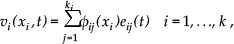
where k_i is the number of modes used to describe the deflection of link i; φ_ij(x_i) and e_ij(t) are the j^th mode shape function and j^th modal displacement for the i^thlink, respectively.

Hence, applying the Lagrangian assumed modes method the dynamic equation of flexible mobile manipulator could be obtained as:

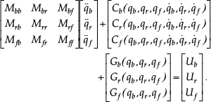
\begin{array}{l} [\begin{matrix} M_{b b} & M_{b r} & M_{b f} \\ M_{r b} & M_{r r} & M_{r f} \\ M_{f b} & M_{f r} & M_{f f} \end{matrix}] [\begin{matrix} {\overset{..}{q}}_{b} \\ {\overset{..}{q}}_{r} \\ {\overset{..}{q}}_{f} \end{matrix}] + [\begin{matrix} C_{b} (q_{b}, q_{r}, q_{f}, {\dot{q}}_{b}, {\dot{q}}_{r}, {\dot{q}}_{f}) \\ C_{r} (q_{b}, q_{r}, q_{f}, {\dot{q}}_{b}, {\dot{q}}_{r}, {\dot{q}}_{f}) \\ C_{f} (q_{b}, q_{r}, q_{f}, {\dot{q}}_{b}, {\dot{q}}_{r}, {\dot{q}}_{f}) \end{matrix}] \\ + [\begin{matrix} G_{b} (q_{b}, q_{r}, q_{f}) \\ G_{r} (q_{b}, q_{r}, q_{f}) \\ G_{f} (q_{b}, q_{r}, q_{f}) \end{matrix}] = [\begin{matrix} U_{b} \\ U_{r} \\ U_{f} \end{matrix}] . \end{array}

(2)

By defining →q = (q_b^T, q_r^T, q_f^T)^T as the vector of generalized coordinate of the system, Eq. (2) can be written in compact form as

M (q) \overset{..}{q} + C (q, \dot{q}) + G (q) = U,

(3)

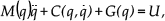
where M is the Inertia matrix, C is the vector of Coriolis and centrifugal forces, G describes the gravity effects and U is the generalized force inserted into the actuator.

3. State-space form of dynamic equation

Consider an n DOFs rigid mobile manipulator with generalized coordinates q = [q_i], i = 1,2,…,n and a task described by m task coordinates r_j, j = 1,2,…,m with m < n. By applying h holonomic constraints and c non-holonomic constraints to the system, r = h + c redundant DOFs of the system can be directly determined. Therefore, m DOFs of the system is remained to accomplish the desired task. As a result, we can decomposed the generalized coordinate vector as q = [q_r q_nr]^T, where q_r is the redundant generalized coordinate vector determined by applying constraints and q_nr is the non-redundant generalized coordinate vector. Also, considering the flexible link manipulators instead of the rigid ones, their related generalized coordinates, q_f, are added to the system; therefore, the overall decomposed generalized coordinate vector of system obtain as q = [q_r q_nrf]^T, where q_nrf is the combination vector of q_nr and q_f.

In this case, the system dynamics can also be decomposed into two parts: one is corresponding to redundant set of variables, q_r and the remained nonholonomic set, q_nrf. That is,

[\begin{matrix} M_{r, r} & M_{r, n r f} \\ M_{r, n r f} & M_{n r f, n r f} \end{matrix}] [\begin{matrix} {\overset{..}{q}}_{r} \\ {\overset{..}{q}}_{n r f} \end{matrix}] + [\begin{matrix} C_{r} + G_{r} \\ C_{n r f} + G_{n r f} \end{matrix}] = [\begin{matrix} U_{r} \\ U_{n r f} \end{matrix}],

(4)

where by considering the second row in order to path optimization procedure leads to

U_{n r f} = A {\overset{..}{q}}_{n r f} + B .

(5)

Using redundancy resolution q_r will be obtained as a known vector in terms of the time (t). Therefore A is obtained as a function of time and q_nrf and B as a function of time, q_r and q̇_nrf.

By defining the state vector as

X = {[\begin{matrix} X_{1} & X_{2} \end{matrix}]}^{T} = {[\begin{matrix} q_{n r f} & {\dot{q}}_{n r f} \end{matrix}]}^{T},

(6)

Eq. (5) can be rewritten in state space form as

\dot{X} = [\begin{matrix} {\dot{X}}_{1} \\ {\dot{X}}_{2} \end{matrix}] = [\begin{matrix} X_{2} \\ N (X) + D (X) U \end{matrix}] = [\begin{matrix} F_{1} \\ F_{2} \end{matrix}],

(7)

where D = M¹ and N= M¹(C(X₁,X₂) + G(X₁)). Then, optimal control problem is determined the position and velocity variable X₁(t) and X₂(t), and the joint torque U(t) which optimize a well-defined performance measure when the model is given in Eq. (7).

4. Formulation of the optimal control problem

Pontryagin's minimum principle provides an excellent tool to calculate optimal trajectories by deriving a two-point boundary value problem. Let the trajectory generation problem be defined as determining a feasible specification of motion, which will cause the robot to move from a given initial state to a given final state. The method presented in this article adapts in a straightforward manner to the generation of such dynamic profiles.

There are known that nonlinear system dynamics stated as Eq. (7) be expressed in the term of states (X), controls (U) and time (t) as

\dot{X} = f (X, U, t)

(8)

Generating optimal movements can be achieved by minimizing a variety of quantities involving directly or not some dynamic capacities of the mechanical system. A functional is considered as the integral

J (u) = \int_{t_{0}}^{t_{f}} L (X, U, t) d t

(9)

where the function L may be specified in quite varied manners. There are initial and terminal constraints on the states:

X (t_{0}) = X_{0} X (t_{f}) = X_{f}

(10)

There may also be certain pragmatic constraints (reflecting such concerns as limited actuator power) on the inputs. For example:

| U (t) | \leq U_{\max} (t)

(11)

According to the minimum principle of Pontryagin (Kirk D.E., 1970), minimization of performance criterion at Eq. (9), is achieved by minimizing the Hamiltonian (H) which is defined as follow:

H (X, U, Ψ, m_{p}, t) = L (X, U, m_{p}, t) + Ψ^{T} f (X, U, t)

(12)

where Ψ(t) = [Ψ₁(t)^T Ψ₂(t)^T]^T is the non-zero costate time vector-function.

Finally, according to the aforementioned principle, stating the costate vector-equation

{\dot{Ψ}}^{T} = - \partial H / \partial X,

(13)

in addition to the minimality condition for the Hamiltonian as

\partial H / \partial U = 0

(14)

\dot{X} = \partial H / \partial Ψ,

(15)

leads to transform the problem of optimal control into a non-linear multi-point boundary value problem.

Consequently, for a specified payload value, substituting obtained computed control equations from Eqs. (14) and Eq. (11) into Eqs. (13) and (15), leads to sixteen nonlinear ordinary differential equations which with sixteen

\begin{array}{l} r_{b} = [\begin{matrix} x_{f} - L_{0} \cos (ϴ_{0}) \\ y_{f} - L_{0} \sin (ϴ_{0}) \end{matrix}] \\ r_{1} = [\begin{matrix} x_{f} + x_{1} \cos (ϴ_{10}) - v_{1} \sin (ϴ_{10}) \\ y_{f} + x_{1} \sin (ϴ_{10}) + v_{1} \cos (ϴ_{10}) \end{matrix}] \\ r_{2} = [\begin{matrix} \begin{array}{l} x_{f} + L_{1} \cos (ϴ_{10}) - v_{1 L} \sin (ϴ_{10}) + x_{2} \cos (ϴ_{210}) - v_{2} \sin (ϴ_{210}) \\ ​ \end{array} \\ y_{f} + L_{1} \sin (ϴ_{10}) + v_{1 L} \cos (ϴ_{10}) + x_{2} \sin (ϴ_{210}) + v_{2} \cos (ϴ_{210}) \end{matrix}] \\ r_{m p} = [\begin{matrix} \begin{array}{l} x_{f} + L_{1} \cos (ϴ_{10}) - v_{1 L} \sin (ϴ_{10}) + L_{2} \cos (ϴ_{210}) - v_{2 L} \sin (ϴ_{210}) \\ ​ \end{array} \\ y_{f} + L_{1} \sin (ϴ_{10}) + v_{1 L} \cos (ϴ_{10}) + L_{2} \sin (ϴ_{210}) + v_{2 L} \cos (ϴ_{210}) \end{matrix}] \end{array}

(16)

boundary conditions given in Eq. (10), constructs a Two Point Boundary Value Problem (TPBVP). Such a problem is solvable with available commands in different software such as MATLAB and MATEMATHICA.

5. Implementation

In this section, implementation is performed for the flexible mobile manipulator consists of a two flexible link manipulator attached at point F(x_f, y_f) on the main axis of a differentially driven vehicle as shown in Figure 1. A concentrated payload of mass m_p is connected to the second link.

Figure 1.

Two-link mobile manipulator with flexible links

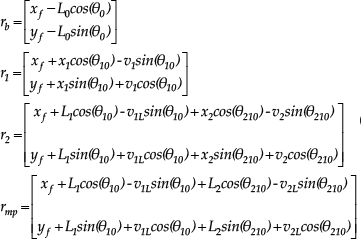
In order to define the mobile manipulator with two flexible links the mechanical system generalized coordinates can be chosen as q = [q_b q_r q_f] = [x_f y_f θ₀ θ₁ θ₂ e₁₁ e₂₁], where q_b = [x_f y_f θ₀] is the base generalized coordinates vector, q_r = [θ₁ θ₂] is the joint angles vector and q_f = [e₁₁ e₂₁] is the vector of link modal displacements. Here, one mode shape per each link is considered to show the simplified model of the system with sensible accuracy. By defining r_b, r₁, r₂ and r_mp as the position vectors of the base, first link, second link and payload respectively, according to Fig. 1, the expressions of these vectors can be expressed as:

where v_iL is the vibration of the end of each link, θ₁₀ = θ₀ + θ₁ and θ₂₁₀ = θ₀ + θ₁ + θ₂. v_i(x_i, t) and v_iL(t) can be expressed as follows:

\begin{array}{l} \begin{matrix} v_{1} = ϕ_{11} (x_{1}) e_{11} (t), & v_{2} = ϕ_{21} (x_{2}) e_{21} (t) \end{matrix} \\ \begin{matrix} v_{1 L} = ϕ_{11 L} e_{11} (t), & v_{2 L} = ϕ_{21 L} e_{21} (t) \end{matrix} \end{array}

(17)

where with considering the simply support mode shape, φ_ij and Ψ can be computed as:

\begin{array}{c} \begin{matrix} \begin{array}{l} ϕ_{i j} (x_{i}) = s i n (\frac{j π x_{i}}{L_{i}}) \\ ϕ_{i j L} = s i n (j π), i = 1 \dots 2 a n d j = 1 \end{array} & ​ \end{matrix} & ​ & ​ \end{array}

(18)

where i and j refer to the number of link and mode shape respectively.

Now, using combined Euler-Lagrange formulation and assumed modes method, the set of system dynamic equations is derived as follows:

[\begin{matrix} m_{11} & m_{12} & m_{13} & m_{14} & m_{15} & m_{16} & m_{17} \\ ​ & m_{22} & m_{23} & m_{24} & m_{25} & m_{26} & m_{27} \\ ​ & ​ & m_{33} & m_{34} & m_{35} & m_{36} & m_{37} \\ ​ & ​ & ​ & m_{44} & m_{45} & m_{46} & m_{47} \\ ​ & ​ & ​ & ​ & m_{55} & m_{56} & m_{57} \\ ​ & ​ & S y m . & ​ & ​ & m_{66} & m_{67} \\ ​ & ​ & ​ & ​ & ​ & ​ & m_{77} \end{matrix}] [\begin{matrix} {\overset{..}{x}}_{f} \\ {\overset{..}{y}}_{f} \\ {\overset{..}{ϴ}}_{0} \\ {\overset{..}{ϴ}}_{1} \\ {\overset{..}{ϴ}}_{2} \\ {\overset{..}{e}}_{11} \\ {\overset{..}{e}}_{21} \end{matrix}] + [\begin{matrix} c_{1} \\ c_{2} \\ c_{3} \\ c_{4} \\ c_{5} \\ c_{6} \\ c_{7} \end{matrix}] = [\begin{matrix} F_{x} \\ F_{y} \\ T_{0} \\ τ_{1} \\ τ_{2} \\ 0 \\ 0 \end{matrix}]

(19)

where because of the motion is in the horizontal plane, the gravity effects, G = (G_b, G_r, G_f) will not taking into account. The position of the end effector in the world reference frame RF_w can be specified with x_e and y_e as shown in Figure 1. Therefore operational coordinated of the end effector can be chosen as E(x_e, y_e) and the end effector degrees of freedom in the Cartesian coordinate system will be m = 2. The rigid system degree of freedom is equal to n = 5, hence the system has redundancy of order r = n - m = 3. Thus, this system needs three additional kinematical constraints for resolving the redundancy problem and guarantees soft and well-organized movement. There is one nonholonomic constraint for the mobile base that undertakes the robot movement only in the direction normal to the axis of the driving wheels:

{\dot{x}}_{f} s i n (ϴ_{0}) - {\dot{y}}_{f} c o s (ϴ_{0}) + L_{0} {\dot{ϴ}}_{0} = 0 .

(20)

Hence, the number of kinematical constraints which must be applied to system for redundancy resolution is decreases to two constraints. In this case, with the previously specification of the base trajectory during the motion, the user-specified additional constraints can be considered. The base position coordinates at point F(x_f, y_f), gives x_f = X_1z and y_f = X_2z. Where, X_1z and X_2z are functions in terms of time. Now, by considering fifth order polynomial function for the base trajectory along a straight-line path from (x_f(0), y_f(0)) to (x_f(t_f), y_f(t_f)) during the overall time t_f the redundancy solution of the system can be complete. Velocity at start and stop time is considered to be zero. According to the base motion, ẋ_f and ẏ_f are known, therefore if the base angle at initial time θ₀(0) be specified, angular position and angular velocity of the base (θ₀(t), θ̇₀(t)), can be determined by solving non-holonomic constraint equations. Note that, the initial base angle is considered to be zero, θ₀(0) = 0.

Now, after resolving the redundancy of the system and remaining the non-redundant set of dynamic equations (Eq. (5)), by defining the state vectors as

\begin{array}{l} \begin{matrix} X_{1} = Q^{T} = {[\begin{matrix} x_{1} & x_{3} & x_{5} & x_{7} \end{matrix}]}^{T}, & ​ \end{matrix} \\ X_{2} = {\dot{Q}}^{T} = {[\begin{matrix} x_{2} & x_{4} & x_{6} & x_{8} \end{matrix}]}^{T} . \end{array}

(21)

The state space form of the dynamic equations of the system can be written as

{\dot{x}}_{2 i - 1} = x_{2 i}, {\dot{x}}_{2 i} = f_{2} (i); i = 1 . . . 4,

(22)

where f₂(i) can be obtained from Eq. (7). These equations must be completed with boundary conditions that consist in the specified initial and final states as

\begin{array}{l} x_{1} (0) = 1.554 rad, x_{3} (0) = 1.998 rad; \\ x_{1} (t_{f}) = - 0.858, x_{3} (t_{f}) = 1.09. \end{array}

(23)

Other boundary conditions are assumed to be zero 0(Korayem M.H. et al., 2009). A performance index is expressed as some functional evaluated over the trajectory. In the presenting paper, the desired path is optimally designed so that the required movement can be achieved while minimum effort is obtained and velocities are bounded at proper magnitude. Hence, the objective function is considered as:

L = \frac{1}{2} (r_{1} u_{1}^{2} {+ r}_{2} u_{2}^{2} + \sum_{i = 1}^{4} w_{i} x_{2i}^{2})

(24)

The main advantage of this cost functional is that the designer can decide on the relative importance among the objective function. For example, in objective function explained in Eq. (24), between the angular velocity and control effort. In this case, by the numerical choice of w_i and r_i the desire movement can be achieved. This, results to choose the most appropriate path among various optimal paths that satisfy the designing requirements. Now, by considering the costate vector as Ψ = [Ψ₁ Ψ₂ … Ψ₈], the Hamiltonian function is formed as

H = \frac{1}{2} (r_{1} τ_{1}^{2} {+ r}_{2} τ_{2}^{2} + \sum_{i = 1}^{4} w_{i} x_{2i}^{2}) + \sum_{i = 1}^{8} ψ_{i} {\dot{x}}_{i},

(25)

where ẋ_i, i = 1,…, 8 can be substituted from Eq. (22). Using Eq. (13), differentiating the Hamiltonian function with respect to the states, result in costate equations as follows:

{\dot{ψ}}_{i} = - \frac{\partial H}{\partial x_{i}}, i = 1, \dots, 8

(26)

The control function in the admissible interval can be computed according to Eq. (14), by differentiating the Hamiltonian function with respect to the torques (τ₁, τ₂) and setting the derivative equal to zero. The actuators that are used in this study are the permanent magnet D.C. motor with the final bound of control as

\begin{array}{l} u_{1}^{+} = τ_{1} - S_{1} x_{11}; u_{1}^{-} = - τ_{1} - S_{1} x_{11} \\ u_{2}^{+} = τ_{2} - S_{2} x_{12}; u_{2}^{-} = - τ_{2} - S_{2} x_{12} \end{array}

(27)

where S_i = (τ_i / ω_mi. τ_i and ω_mi are the stall torque and maximum no-load speed of i^th motor respectively.

Typically, applying the Pontryagin's minimum principle results a two-point boundary value problem. Indeed, substituting the computed control equations in the state and costate equations (22) and (26) yields a 4n ordinary differential equation, where the functions X (t) and Ψ(t) must satisfy the 4n boundary conditions.

Numerical libraries offer efficient computing codes for solving non-linear problems of this type. We used the routine BVP4C of the MATLAB® library, which is based on the collocation method. The details of the numerical technique used in MATLAB® to solve the TPBVP are given in (Shampine L. F. et al).

6. Illustrative examples

In this section, simulations are carried out at two cases. In the first case, path planning is performed for the different values of penalty matrices. In the second case, simulation is done for the high stiffness mobile robot and results are compared with the rigid mobile robot (Korayem M.H. et al., 2009). The necessary parameters used in the simulations are summarized in the Table 1.

Table 1.

Simulation Parameters

Parameter	Value	Unit
Length of Links	L₁ = L₂ = 0.5	m
Mass of Links	m₁ = 5; m₂ = 3	kg
Mass of Base	m_b = 1	kg
Moment of Area of Links	I₁ = I₂ = 5e-11	m ⁴
Module of Elasticity of Links	E₁ = E₂ = 2e11	kg.m²
Max. no Load Speed of Actuators	w_s1 = 6.45; w_s2 = 2.4	rad/s
Actuator Stall Torque	τ_s1 = 34.67; τ_s2 = 12.21	N.m

The load must be carried from an initial point with coordinate (x_e = 0.3m, y_e = 0.5m) to the final point with coordinate (x_e = 2.45m, y_e = 0.5m). The optimal trajectory between these two points during the overall time t_f =1.9 second is desired. It should be noted that the final load position is not feasible without the base motion. Simultaneously, the mobile base is initially at point (x_f = 0.75m, y_f = 0.2m, θ_f = 0) and moves to final position (x_f = 1.6m, y_f = 0.5m). L₀ is supposed to be 40 cm. (Korayem M.H. et al., 2009).

In the first case, the payload is considered to be 2 kg. The purpose is to find the optimal path of payload in such a way that the more suitable amount of control value be applied and the angular velocity values of motors be bounded in ±1.5 rad/s.

By considering penalty matrices as: w₁ = w₂ = 0.1, w₃ = w₄ = 0 and r₁ = r₂ = diag (0.01) the first path with appropriate amount of control value are determined, but the angular velocities are greater than |1.5| rad/s. Hence, reducing the maximum velocity magnitude must be considered. Therefore, for decreasing the joint velocities, at cost functional defined in the Eq. (24) the penalty matrix corresponding to them must be increased. A range of values of W = (w, w, 0, 0) used in simulation are given in Table 2. r_i remains without changes.

Table 2.

The values of w used in the simulation

case	1	2	3	4
w	0.1	1	10	200

End effector trajectories in the XY plane are shown in Figure 2. Figure 3 shows the angular positions of joints with respect to time. This graph shows that by increasing the w, the angular position change to approach approximately to a straight line. Figure 4 shows the angular velocities of the first and second joints. It can be found that by increasing the w, the final values of angular velocity reduce from −2.3 rad/s to −1.5 rad/s. By growing the w, the angular velocities reduce greatly for the first to second cases whereas at the third case a little reduction has been occurred in spite of great increase in w.

Figure 2.

End effector trajectory in XY plane

Figure 3.

Angular positions of joints

Figure 4.

Angular velocities of joints

The computed torqueses are plotted in Figure 5. As it can be seen, increasing the w causes to raise the torques, so that for the last case the torque curves reach to their bounds at the beginning and end of the path. This result is predictable, because, increasing the w decreases the proportion of r_i and the result of this is increasing the control values.

Figure 5.

Torques of motors

Mode shapes are plotted in Figure 6, shows the flexible nature of the system in case 3. Finally, arm motions with related end effector and base trajectories in this case are plotted in Figure 7.

Figure 6.

Mode shapes of links

Figure 7.

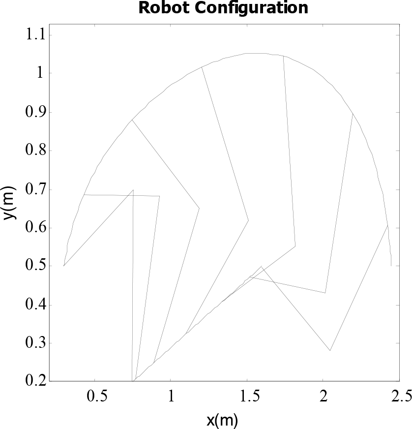
robot configuration in the Cartesian plane

It can be concluded that, the first path is the optimal path with the least control values, whereas its angular velocity is the largest magnitude and the last path is the optimal path with the smallest amount of velocities, while its control values is the largest amount. Finally, for the considered problem, the optimal path is the third path, which its velocity magnitude is bounded in ±1.5 rad/s interval and the torque values is the lowest.

In contrast, the optimal path with lower effort with greater velocity and the optimal path with greater effort with lower velocity are obtained using this method; accordingly, based on the objective contrast principle, there is not a unique solution that satisfies all the desired objectives simultaneously. Consequently, in this method, designer compromises between different objectives by considering the proper penalty matrices and obtain the finest path that appropriately cope with the designing requirements.

In order to verify the validity of the study, the case proposed in literature is developed with elastic behavior in links (Korayem M.H. et al., 2009). The rational comparison can be made between rigid manipulator and flexible ones, by increasing the stiffness at the flexible link. It leads to reduce the flexible manners of the system and approaches it into rigid links. Hence, the simulation is done by increasing the moments of area of each link in previous case study from 1e-11 to 6e-9. The payload is considered to be 20.2 kg (Korayem M.H. et al., 2009). Figures 8 –10 show the comparison between angular positions, angular velocities and torque curves in the rigid and high stiffness case, respectively; as seen from these figures, both simulation outputs are in a good agreement, which validates the method studied in this paper. Finally, mode shapes in this case is shown in Figure 11.

Figure 8.

Angular positions of joints

Figure 9.

Angular velocities of joints

Figure 10.

Torque curve of actuators

Figure 11.

Mode shapes of links 1 and 2

7. Conclusion

In this paper, path planning problem of a flexible mobile manipulator in point-to-point motion is formulated based on the open-loop optimal control approach. The first objective of paper is to state the dynamic optimization problem under a quite generalized form for the optimality solution that commonly encountered in the field of path planning of mechanical manipulators. The second objective consists in developing the method for optimizing the applicable case studies, which results. First, concepts such as redundancy and link flexibility are explained and the general flexible links mobile manipulator is modeled. Then, Pontryagin's minimum principle is called for a Hamiltonian state equations and optimal path with general objective function is designed based on TPBVP. Finally, the method is implemented on two case studies and obtained results are compared with those reported in literature. It illustrates the power and capability of the method to overcome the high nonlinearity nature of the optimization problem in spite of using complete form of the obtained nonlinear equations. Highlighting the main contribution of the paper can be presented as:

The proposed approach can be adapted to any general serial manipulator including both non-redundant and redundant systems with link flexibility and base mobility.

In this approach the nonholonomic constraints do not appear in TPBVP directly, unlike the method given in literature (Mohri A. et al. 2001; Furuno S. et al. 2003).

This approach allows completely nonlinear states and control constraints treated without any simplifications.

This paper is the first path generation study that applied at the flexible mobile manipulators with un-predefined trajectory of end-effector.

The obtained results illustrate the power and efficiency of the method to overcome the high nonlinearity nature of the optimization problem, which with other methods, it may be very difficult or impossible.

In this method, boundary conditions are satisfied exactly, while the results obtained by ILP method have a considerable error in final time.

In this method, designer is able to choose the most appropriate path among various optimal paths by considering the proper penalty matrices.

The optimal trajectory and corresponding input control obtained using this method can be used as a reference signal and feed forward command in the closed-loop control of such manipulators.

References

Bertolazzi

Biral

& Da Lio

(2005). Symbolic– numeric indirect method for solving optimal control problems for large multibody systems. Multibody System Dynamics, Vol. 13, No. 2, pp. 233–252

Bessonnet

& Chessé

(2005). Optimal dynamics of actuated kinematic chains, Part 2: Problem statements and computational aspects. European Journal of Mechanics A/Solids, Vol. 24, pp. 472–490

Callies

& Rentrop

(2008). Optimal control of rigid-link manipulators by indirect methods. GAMM-Mitt., Vol 31, No. 1, pp. 27–58

Chen

M. W.

& Zalzala

A. M. S.

(1997). Dynamic Modelling and Genetic. Based Trajectory Generation for Non-Holonomic Mobile Manipulators. Pergamon Journal of Control Engineering Practice. Vol. 5, No. 1, pp. 39–48

Furuno

Yamamoto

& Mohri

(2003). Trajectory planning of mobile manipulator with stability considerations. Proceedings of IEEE International Conference on Robotics and Automation, pp. 3403–3408

Green

& Sasiadek

J.Z.

(2004). Dynamics and Trajectory Tracking Control of a Two-Link Robot Manipulator. Journal of Vibration and Control, Vol. 10, No. 10, pp. 1415–1440

Hull

D.G.

(1997). Conversion of optimal control problems into parameter optimization problems. Journal of Guidance and Control Dynamics. Vol. 20, No 1, pp.57–60

Kim

J.S.

& Uchiyama

(2003). Vibration mechanism of constrained spatial flexible manipulators. JSME International Journal. Series C. Mechanical Systems machine Element Manufacturing, Vol. 46, No.1, pp. 123–128

Kirk

. (1970). Optimal control theory, an introduction, In: Prentice-Hall Inc., Upper Saddle River, New Jersey.

10.

Korayem

M. H.

& Ghariblu

(2004). Analysis of wheeled mobile flexible manipulator dynamic motions with maximum load carrying capacities. Robotics and Autonomous Systems, Vol. 48, No. 2–3, pp. 63–76

11.

Korayem

M.H.

Heidari

& Nikoobin

(2008). Maximum Allowable Load of Flexible Mobile Manipulators Using Finite Element Approach. International Journal of advanced manufacturing technology. Vol. 36, No.5–6, pp. 606–617

12.

Korayem

M.H.

Nikoobin

& Azimirad

(2009). Maximum Load Carring Capacity of Mobile Manipulators: Optimal Control Approach. Robotica, Vol. 27, No. 1, pp. 147–159

13.

Matsuno

& Hatayama

(1999). Robust Cooperative Control of Two Two-Link Flexible Manipulators on the Basis of Quasi-Static Equations. International Journal of Robotic research. Vol. 18, No. 4, pp. 414–428

14.

Mohri

Furuno

& Yamamoto

(2001). Trajectory planning of mobile manipulator with end-effector's specified path. Proceedings of IEEE International Conference on Intelligent Robots and systems, pp. 2264–2269

15.

Park

K. J.

(2004). Flexible robot manipulator path design to reduce the endpoint residual vibration under torque constraints. Journal of Sound and Vibration. Vol. 275, pp. 1051–1068

16.

Papadopoulos

E. G.

& Poulakakis

(2001). Planning and Obstacle Avoidance for Mobile Robots. Proceedings of the IEEE International Conference on Robotics and Automation, Seoul, Korea

17.

Sentinella

M. R.

& Casalino

(2006). Genetic algorithm and indirect method coupling for low-thrust trajectory optimization. Proceedings of 42nd AIAA/ASME/SAE/ASEE Joint Propulsion Conference and Exhibit, Sacramento, Jul 2006

California, USA

18.

Seraji

(1998). A unified approach to motion control of mobile manipulators. International Journal of Robotic Research, Vol. 17, No. 12, pp.107–118

19.

Shampine

L. F.

Reichelt

M. W.

& Kierzenka

(2000). Solving boundary value problems for ordinary differential equations in Matlab with bvp4c, available from : http://www.mathworks.com/bvptutorial, Accessed:2000/10/26

20.

Subudhi

& Morris

A.S.

(2002). Dynamic Modelling, Simulation and Control of a Manipulator with Flexible Links and Joints. Robotics and Autonomous Systems, Vol. 41, pp. 257–270

21.

Sun

Sharf

, & Nahon

(1999). Stability Analysis of the Force Distribution Algorithm for Flexible-Link Cooperating Manipulators. Mechanism and Machchine Theory. Vol. 34, pp. 753–763

22.

Tanner

H. G.

(2003). Nonholonomic Navigation and Control of Cooperating Mobile Manipulators. IEEE Transcation on Robotic and Automation. Vol. 19, No. 1, pp. 53–61

23.

Wilson

D. G.

Robinett

R. D.

& Eisler

G. R.

(2004). Discrete Dynamic Programming for Optimized Path Planning of Flexible Robots. Proceedings of the International Conference on Intelligent Robot and Systems, pp. 2918–2923.

24.

Yue

Tso

S. K.

& Xu

W. L.

(2001). Maximum dynamic payload trajectory for flexible robot manipulators with kinematic redundancy. Mechanism and Machine Theory, Vol. 36, pp. 785–800

25.

Zhu

S.S.

& Lee

T.H.

(1999). Simulation studies of tip tracking control of a single-link flexible robot based on a lumped model. Robotica. Vol. 17, pp. 71–78

Path Planning of Mobile Elastic Robotic Arms by Indirect Approach of Optimal Control

Abstract

Keywords

1. Introduction

2. Modeling of a general mobile manipulator with multiple flexible links

3. State-space form of dynamic equation

4. Formulation of the optimal control problem

5. Implementation

6. Illustrative examples

7. Conclusion

References