A Robust Alternative to Critical Peak Pricing for Electricity Using Distributed Energy Storage

Abstract

This article addresses the classic problem of pricing electricity on peak-load days to lower the system peak and meet the conditions for long-run efficiency. It is assumed implicitly that the wholesale market is monitored to ensure that the price equals the short-run marginal cost of supply. Distributed storage can be used to shift load and/or provide ramping services, and when the supply is inelastic, the storage is used mainly to shift load and reduce the system peak. However, our analysis focuses on the case when supply is elastic on a peak-load day, and consequently, the storage is used mainly for ramping and is not long-run efficient. To overcome this problem, Critical Peak Pricing (CPP) is evaluated as the conventional way to provide the incentive needed for storage to shift load away from the peak. Our main contribution is to demonstrate that the uncertainty of wind generation and price undermines the performance of CPP, and we propose a better, robust storage strategy. Daily simulations of wind generation on the peak-load day are used to determine the wholesale electricity price using a linear supply curve of net-load plus a stochastic residual. We argue that meeting the established reliability standard for "system adequacy" of only failing one-day-in-ten-years corresponds to covering the worst case, with the lowest realized wind generation, in 1000 simulations. Using this standard, the robust strategy maximizes the attainable peak reduction, and this is nearly three times larger than the corresponding reduction using the CPP strategy. The CPP strategy stabilizes the savings earned in the wholesale market, but all ramping requirements must be provided by the system operator. In contrast, the robust strategy provides the ramping needed to stabilize peak net-load, but the savings in the wholesale market are lower and much riskier. Since the owners of storage are likely to prefer the CPP strategy, we conclude that regulators should focus on ways to reduce the ramping requirements for adequacy by, for example, using the more accurate forecasts of wind generation associated with a receding-horizon optimization.

1. Introduction

This article addresses an old problem together with a new problem that is growing rapidly in importance. The old problem is how to provide the economic incentives needed for customers to reduce their purchases of electric energy from the grid during peak periods. To be consistent with long-run efficiency, the annual peak load should be lower to reduce the amount of installed generating capacity needed for system adequacy. In electricity markets where the wholesale price of energy is determined by the short-run marginal cost of generation, the price incentives are inadequate when the supply function is elastic. Consequently, it is more long-run efficient to augment the energy prices during peak-load periods using, for example, Critical Peak Pricing (CPP). The performance of CPP is evaluated in Section 4 of the article, and a summary of the literature on these topics is presented in Section 2.

The new problem is the increasing uncertainty about actual system conditions in a day-ahead market caused by the growth of generation from renewable sources. Although planning by vertically integrated electric utilities has always considered uncertainty in the form of equipment failures (contingencies), the probability of a contingency occurring is small. The standard practice is to have generating capacity on standby (reserves) to cover these contingencies. However, the variability of renewable energy sources is an inherent characteristic and not a rare event. Consequently, generating capacity and demand response must be able to offset this variability by continuously providing the up and down ramping needed to maintain operating reliability. Our analysis assumes that the generation from wind farms is the only source of uncertainty for committing units in a day-ahead market at the wholesale level. Other sources that may affect the units committed, such as contingencies and the uncertainty of load, are not considered.

Energy storage systems (ESS) are a valuable resource for improving operations on a grid. Storage can mitigate the variability of renewable generation, and distributed storage can also modify the daily profile of purchases from the grid by shifting load from one hour to another. For example, on sunny days in parts of California, there is more than enough solar generation to meet all load during the day, but in the evening, the net-load increases as the solar generation decreases. This situation requires a substantial amount of up-ramping capacity to keep the lights on. Moreover, the lack of solar energy production at night, low energy production from wind energy towards the end of summer afternoons and higher temperatures can increase the demand, shifting load from the afternoon to later in the day. By charging ESS during the day and discharging it in the evening, the up-ramping needed from conventional generating units would be much lower. In this example of solar generation, shifting load and providing up-ramping complement each other. However, mitigating the variability of wind generation is different because generally shifting load competes with ramping for how storage capacity is used. This is particularly important on peak-load days if the day/night price differentials are small so that the economic incentive to shift load is also small. In this situation, it is appropriate to consider using CPP.

The main focus of this work is on evaluating how different strategies for managing distributed storage perform when supply is elastic, the price incentives for shifting load are inadequate and there is a substantial amount of uncertainty about the level of wind generation. We assume the manager of the distributed storage is an independent aggregator who is not affiliated with operations on the grid. ¹ The objective of the aggregator is to submit bids into the wholesale market to minimize the expected daily cost of purchases of energy subject to meeting the customers' demand for energy services throughout the day. We assume no aggregator is large enough to be marginal and therefore they behave as price-takers. In our application, deferrable demand provides thermal storage for space cooling. This form of distributed storage is chosen because air conditioners represent a large portion of the annual peak load, and the capital cost of thermal storage is relatively low compared to the cost of batteries. Please refer to Jeon et al. (2015) for further details on the specifications of thermal storage. In the empirical examples, the hourly loads for a peak-load day on the New York and New England systems are treated as known, and wind generation is represented by a simple time-series model presented in Appendix A. Consequently, Net-Load = Total Load - Renewable Generation is stochastic. An important reason for having storage is to reduce the peak net-load and the associated capital cost of the installed generating capacity needed for adequacy, and there is a basic trade-off between these savings and the capital cost of the storage capacity needed to do it.

When the uncertainty of wind generation is ignored by using deterministic forecasts of wind generation, it is straightforward to derive the optimum conditions for using storage to shift load because ramping is not an issue. This deterministic problem is discussed in Section 3. However, once uncertainty is considered explicitly in Section 4, the problem becomes more complicated. The optimum bidding strategy for an aggregator, who faces stochastic price forecasts for the next day, is to determine price thresholds for charging and discharging storage. For any hour, the probabilities of charging, discharging are determined. The probability of neither charging nor discharging implies that storage is available for ramping. When the supply curve is elastic, the probability of ramping is large and the amount of load shifted is small. In this situation, introducing CPP reestablishes the price incentives for shifting more load, and the forecasted peak reduction shows that CPP is a satisfactory way to increase long-run efficiency. This conclusion is, however, misleading because the forecasted peak reduction may violate the standards for adequacy.

The main contribution of this article is to evaluate how well the storage strategies perform with different realized levels of wind generation and price. A simulation of 1,000 realizations (days) is conducted to do this. The results show that the forecasted peak reductions are a misleading metric of performance. The up-ramping needed at the peak must be considered explicitly to get a metric that does meet the standard for system adequacy, and the worst case with the lowest realized wind generation in 1000 simulations meets this standard. In general, a reduction in the forecasted peak load can be much larger than the "attainable" reduction needed for adequacy. We argue that given the increasing uncertainty associated with renewable generation, the traditional use of the Forecasted Peak Net-Load to determine the amount of conventional generating capacity needed for adequacy should be replaced by Forecasted Peak Net-Load + Up-Ramping. This is particularly important when distributed storage is available because the way this storage is managed has a direct effect on the amount of up-ramping needed.

For any given storage strategy that submits optimum bids, the two price thresholds remain the same for all 1000 realizations. As a result, the charging/discharging profile for storage, and the corresponding peak net-load, can be determined for each realization. We define ΔPeak = Max[At-tainable Peak Reduction] = Min[Realized Peak Reduction] in the 1000 realizations for a given storage strategy. All four of the storage strategies evaluated have a forecasted peak reduction that is substantially larger than the corresponding minimum simulated reduction (ΔPeak). In particular, the CPP strategy has a disappointingly low ΔPeak because the highest simulated net-load occurs outside the CPP period. For a given amount of storage capacity, a major objective for reducing total system costs on a peak-load day is to find the strategy that makes ΔPeak as large as possible. We propose a "Robust Heuristic" strategy that discharges storage to reach a target net-load that does maximize ΔPeak and meet the standard for adequacy. ² This is accomplished by having enough stored energy to cover the worst realization with the lowest simulated wind generation.

Using the CPP strategy, storage is always fully discharged during the expensive CPP period. Consequently, the costs of purchased energy during the CPP period are much lower and less volatile using the CPP strategy than the robust strategy. In this sense, there is a substantial opportunity cost from using storage to maximize ΔPeak. We argue in Section 4.6 that the owners of storage are likely to prefer the CPP strategy to the robust strategy, and the conclusions in Section 5 offer some advice for regulators. A review of the literature in Section 2 follows.

2. Background and Literature Review

The economic problem of determining the efficient level of infrastructure to support demand that causes congestion at certain times is relevant for many industries. For example, Vickrey (1963) discusses pricing in transportation systems, where a carefully set peak/off-peak differential can improve the overall utilization of roads and reduce the congestion, and he foretells the implementation of congestion pricing in urban areas, e.g., London. Moreover, the external costs of congestion during peak hours are not paid by the users (Vickrey, 1969), leading to sub-optimal and excess investment in infrastructure (e.g., new highways and airports, natural gas storage and pipelines, bandwidth capacity in a communications systems). The proposed solutions include cost-sharing schemes to account for externalities that converge towards efficient equilibria (e.g., Liu et al., 2015).

The study of price design has occupied economists for a long time, and in the case of the electric grid, this predates the restructuring of the industry in the 1990s when most utilities were vertically integrated and generation was regulated. Generally, the issue of pricing for peak demand occurs for commodities with uneconomical storage costs, uncertain demand and non-convexities in production. In these second best situations, a generally accepted method to handle the problem is to use Ramsey pricing, charging higher prices to more inelastic customers. Before looking at the work focused on electricity pricing, recall that there are three main functions that the pricing mechanism plays:

1. Raise revenues to pay the costs of supplying a good (e.g., electricity). Hence they should be revenue adequate (at least in expectation),

2. Create financial incentives to align production and consumption decisions efficiently,

3. Distribute the costs amongst the customer base.

In meetings of the European econometric society held in Louvain over 70 years ago, Boi-teaux discussed welfare issues associated with selling utility (public service) goods at marginal cost in imperfect environments, given that these were regulated monopolies. Boiteaux's article was first published in French in 1949 and later published in English Boiteux (1960). In it, he discusses the issues of uncertain demand and non-convexities in production stemming from the fixed capacity of the production plants and how this affects the pricing of the good produced.

Classical work by Steiner (1957) proposed a model to distinguish between the marginal costs on-peak and off-peak, calculating the welfare gains compared to charging an average cost for all time periods. Turvey continued this line of research and dedicated Chapter 7, "Optimal Pricing Through Time" of his textbook (Turvey, 1971) to this problem. He proposed covering the capital cost of building additional generating capacity with a surcharge on the price above the short-run marginal cost during peak-load periods.

For situations with different technologies under convexity cost assumptions, not serving demand may be optimal Crew and Kleindorfer (1976), compensating for the rationing cost incurred. Mitchell et al. (1978) in collaboration with staff at Los Angeles Department of Water and Power also studied this problem, including considerations relevant at the time (e.g., inflation), and they evaluated different classical pricing schemes, including Ramsey pricing. The book includes a study of tariffs in Norway, Sweden, France, England and Wales, West Germany and Finland, and proposes a pricing strategy for the United States. Assuming affine cost functions with both uncertain supply and demand, Chao (1983) show that it is not necessary to know the joint distributions of these uncertainties to determine the optimal peak pricing strategies. Optimal pricing and investment rules for priority pricing are examined in Chao and Wilson (1987), with services that are differentiated by the priority of service, and customers paying higher prices for a higher priority.

Other alternative nonlinear pricing strategies to internalize the capacity needed during peak periods have been studied Wilson (1993), drawing parallels with other industries with peaky demands that require spare capacity, and illustrating this with several examples from the electricity industry, including Ramsey pricing and tariffs in France from Électricité de France (EDF). The work in Chao (1983) is extended in Kleindorfer and Fernando (1993), differentiating the cost of disruption for consumers from the cost of rationing for system operators and examining the welfare implications. Before electricity markets were "deregulated" in the US, Crew et al. (1995) surveyed the peak-load pricing theory up to the article's publication time in 1995. Borenstein and Holland (2005) analyzed alternatives to real-time prices, including capacity subsidies. The article shows how flat-rate tariffs lead to welfare losses and do not attain even second-best optimal allocation for both the short and long run, leading to shortfalls in investment in new capacity. In a paper in honor of Alfred Kahn, Joskow and Wolfram (2012) reviewed advances in peak-load pricing from the time that Kahn first implemented marginal cost pricing in New York State in the 1970s, and reviewed the future outlook, including studies that quantified the potential effects of separating active customers from passive customers. A review by Oren (2013) drew attention to numerous initiatives suggested in the 1980s to manage peak electricity demand, including programs in France, Massachusetts, Oklahoma and California, as well as the past literature including Chao and Wilson (1987). Oren proposed a menu of services (segments) with different qualities associated with each one to incentivize demand response. The pricing for a contract depends on the generating capacity needed for each segment. Blonz (2016) estimated the response that small commercial and industrial customers have to Critical Peak Pricing (CPP), and showed that by increasing the peak/off-peak differentials, while also limiting the number of eligible days, CPP can obtain 80 percent of the benefits of real-time pricing.

In a recent paper, Borenstein and Bushnell (2018) quantified deviations between retail prices and the short-run marginal cost of supply across different regions of the US. The authors find that generally the coasts (e.g., California, New England, New York) pay prices above the social marginal costs, whereas the upper central Midwest (e.g, Dakotas, Nebraska, Minnesota) have prices that do not cover the social marginal costs and are in fact negative, and they also calculated the dead-weight losses due to these differences. Cui and Li (2018) study optimal pricing for Time-of-Use (TOU) rates, considering strategic interactions between the load serving entities (LSE) or utilities in charge of provision of energy services and the customers being served. The authors find Pareto-improving equilibria, with customers naturally segregating into groups, reducing the search space and complexity of managing the TOU program. In Eisenack and Mier (2019), the authors studied the effect of non-dispatchability on the classical results summarized in Crew et al. (1995), analyzing the case in which three different technologies are available, a non-responsive, non-dispatchable technology, a partially responsive technology (e.g., non-flexible thermal generation), a very responsive technology (e.g., combined-cycle gas generation). In their comparative study, the authors found that the optimum generation portfolios only select a limited set of technologies, with the non-dispatchable technology dominating, and sometimes, the responsive technology is included.

The papers cited above address the classic problem of peak-load pricing, and the focus turns now to the new problems associated with the uncertainty of renewable generation and the availability of storage capacity. Steffen andWeber (2013) examine the amount of efficient storage capacity needed to meet a residual load duration curve with high penetrations of wind and solar power. They show that a higher price of CO2 and a steeper load duration curve, due to a high share of renewable sources, increase the efficiency of storage capacity as a way to lower the total cost of supplying power. Durmaz (2014) analyzes the welfare improvements when storage is added to a power system with renewable sources using an the economy-energy model. The study shows that energy storage does not improve welfare when the share of renewable energy is low and the marginal cost function of fossil generation is linear. In contrast, storage contributes more when both the intermittency of renewable generation and the convexity of the marginal cost of fossil generation are higher. Helm and Mier (2021) study the optimal subsidy scheme for renewable generation and storage by examining their contribution to reducing the price of energy and the amount of fossil fuel generation. They conclude that the subsidy for storage should be negative when the penetration of renewable generation is low, because storage is charged using fossil fuel energy, implying that more dirty energy is used due to the round-trip inefficiency of storage. In contrast, when the share of renewable generation is high, storage should be subsidized because it charges using renewable energy and discharges during hours with low renewable generation, displacing fossil fuel generation. This paper shows that the profitability of storage will be higher when the share of renewable generation is high, because storage benefits more from price arbitrage due to the larger range of daily prices. In addition, there are benefits from reducing the amount of fossil fuel generation. Ekholm and Virasjoki (2020) study market power and competition between storage and renewable energy in a power system with 100% renewable energy penetration. Elastic demand and storage are the only flexible sources. The paper claims that consumers will benefit from the market power of storage because zero prices will occur more frequently when generation from renewable sources is high, and this will lower the revenue of renewable sources. Geske and Green (2020) address a similar problem to the one analyzed in this paper, and our results are consistent with the subtitle of their paper, "It is costly to avoid outages". The model in Geske and Green (2020) treated net-generation as stochastic and used a Markov-process to represent the uncertainty of the hourly net-load in Germany. Storage can be used to shift the load from expensive periods to less expensive periods, but the need for precautionary storage must also be considered to avoid paying VOLL when there are unexpectedly long periods with low levels of renewable generation. The authors conclude that if the need for precautionary storage is ignored, the cost saved by storage will be overestimated. The need for generation flexibility in the presence of uncertain renewable generation is examined by Mier (2021). In this paper, it is assumed that prices are allowed to rise to scarcity levels.

A recent paper by Schmalensee (2022) analyzed the role of storage as a way to manage the "duck curve" in California. By charging storage during the day when there is abundant solar generation, the storage can be discharged in the evening to reduce the amount of ramping needed from conventional generating units when the sun goes down. The analysis uses a two-period model (night and day) that treats both the solar generation and the load as stochastic inputs. Optimum short-run and long-run efficiency conditions are derived in an "energy only" market that allows the price of electricity to occasionally equal the Value-Of-Lost-Load (VOLL). Customers pay the real-time prices.

In contrast, our analysis assumes that the wholesale energy market is similar to those in the Northeastern US that are closely monitored to keep prices equal to the short-run marginal cost, and are also subject to a price cap that is much smaller than the VOLL. We use the established industry standard for reliability to determine the requirements for system adequacy rather than relying on the real-time price occasionally reaching the VOLL. ³ This standard corresponds to having enough storage capacity to cover the worst case situation, with the lowest realized wind generation, in 1000 simulated days. Since adequacy is not determined by the high price of VOLL in our analysis, we follow the conventional approach proposed by (Turvey, 1971) and evaluate the performance of Critical Peak Pricing as an alternative way to encourage the shifting of load away from peak-load periods. We also make a clear distinction between the statistical properties of the forecasted net-load, that is used to determine the bids/offers for managing distributed storage optimally, ⁴ and the realized net-load, that is used in the simulations to evaluate how well each storage strategy performs. A description of our analytical methods follows in Sections 3 and 4.

3. An Economic Assessment of Storage: Deterministic Case

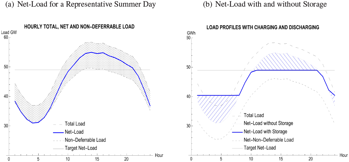
In this section, we present a model for evaluating the use of storage in a deterministic case when there is no uncertainty about the load and renewable generation. ⁵ The analysis is based on the hourly loads for a peak-load day in the northeastern U.S., corresponding to the areas managed by the New York Independent System Operator (NYISO) and ISO New England (ISO-NE). To avoid using large numbers, the power and energy quantities are GW and GWh, but the prices conform to the standard $/MWh for the wholesale price of energy and $/MW for the capital cost of generating capacity. Figure 1(a) shows the hourly profile of the Total Load (GW) on a hot summer day that includes the annual peak and sets the planning requirements for the amount of installed generating capacity needed to meet Generation Adequacy. ⁶ The Net-Load (GW) = Total Load - Renewable Generation, and corresponds to the level of load that must be covered by conventional generation. The analysis assumes that all renewable generation comes from wind turbines, represented by a simple time-series model that will be used in the next section to determine the uncertainty of the Net-Load. In addition, storage capacity is represented by the deferrable demand from using thermal storage to replace air-conditioners for space cooling. The deferrable demand is specified to be 15 percent of the Total Load, implying that the Non-Deferrable Load (GW) is 85 percent of the Total Load, and the shaded area in Figure 1 corresponds to the deferrable demand (GWh).

Figure 1:

The Effect of Storage on Net-Load

We make no distinction between the terms "storage" and "deferrable demand," and both of them represent distributed storage in this analysis. The main difference between them is that the amount of energy discharged from battery storage for a given hour is limited by the maximum rate of discharge, but the limit for deferrable demand is given by:

$$\min \left\{\mathrm{Maximum}\mathrm{rate}\mathrm{of}\mathrm{discharge},\mathrm{Amount}\mathrm{of}\mathrm{deferrable}\mathrm{demand}\mathrm{needed}\right\}.$$

(1)

For example, when thermal storage is used to replace air-conditioning, the energy discharged cannot exceed the amount of cooling needed.

Figure 1(b) illustrates the effect of using storage to modify the daily load profile. The Net-Load Without Storage becomes the Net-Load With Storage, and the Net-Non-Deferrable Load is given by:

$$\mathrm{Net}-\mathrm{Non}-\mathrm{Deferrable}\mathrm{Load}=\mathrm{Non}-\mathrm{Deferrable}\mathrm{Load}-\mathrm{Wind}\mathrm{Generation}.$$

(2)

The ratio of the increased amount of off-peak energy purchased to the on-peak energy displaced is fixed by the round-trip efficiency of storage. Consequently, the basic economic tradeoff in capital costs is between the savings in the amount of installed generating capacity needed for adequacy from reducing the peak net-load, and the amount of storage capacity needed to hold the stored energy, and

$$\begin{array}{l}\mathrm{Reduction}\mathrm{of}\mathrm{the}\mathrm{Peak}\mathrm{Net}-\mathrm{Load}=\max \left\{\mathrm{Net}-\mathrm{Load}\mathrm{Without}\mathrm{Storage}\right\}\\ -\max \left\{\mathrm{Net}-\mathrm{Load}\mathrm{With}\mathrm{Storage}\right\}.\end{array}$$

(3)

To simplify the analysis for the deterministic optimization, we set the model to have more deferrable demand available than the amount needed to minimize the total daily cost of purchasing energy, and the discharge rate is also not binding. Placing binding limits on charging and discharging becomes important for the stochastic optimization in the next section when storage can also be used for ramping.

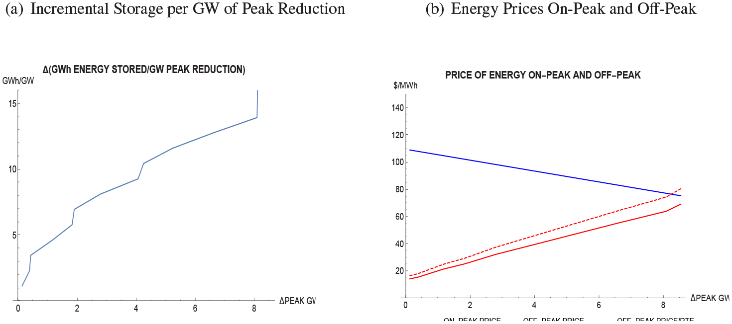
Inspection of Figure 1(b) implies that the amount of storage needed (GWh) per GW of peak load reduction is a monotonically increasing function, implying that the marginal capital cost of the storage needed is also increasing. This tradeoff is illustrated in Figure 2(a), and the GWh of storage needed per additional GW of peak reduction increases from approximately one to fourteen. When the reduction of the peak net-load is greater than 9 GW, the daily profile of net-load is essentially flat.

Figure 2:

The Effect of Peak Reductions on Storage Capacity and Energy Prices

For simplicity, the following linear supply function is specified to determine the wholesale price of energy for a given level of net-load:

$$\mathrm{Price}\left(\$/\mathrm{MWh}\right)=-110+4\times \mathrm{Net}-\mathrm{Load}\left(\mathrm{GW}\right).$$

(4)

Using this specification to determine prices for the Net Load in Figure 1(a), the average price is $74/MWh and the hourly prices range from $22/MWh to $113/MWh. The corresponding prices of energy for incremental reductions in the peak net-load are shown in Figure 2(b). Basically the maximum on-peak price decreases and the minimum off-peak price increases as the daily load profile gets flatter.

Definition 1 Notation at the System Level

Variable	Description
Τ	: {1, . . . ,T}, set of time periods
AA	: Intercept of the linear supply function
BB	: Slope of the linear supply function
B(HL, LL)	: Benefits of modifying the high load and low load energy profiles
ct, dt ∈ℝ+	: Charging and discharging in period t ∈ Τ
D t	: Level of deferrable demand in period t ∈ Τ
D(L)	: Incremental GWh of energy deferred per GW of peak reduction
HL	: New high load with energy storage capacity
KS	: Capital cost of storage capacity adjusted to the analysis period, $/MWh
KG	: Capital cost of generating capacity adjusted to the analysis period, $/MW
KCS(L)	: Total capital cost of storage
KCG(PL, HL)	: Savings in the capital cost of installed generating capacity
L, L t	: Demand in period t ∈ Τ (GW)
LL	: New low load with energy storage capacity
ML	: Minimum Load
NL	: Hourly Net Load without storage, t = 1, 2, . . . , 24
NLS t	: Net Load with energy storage capacity
P(L)	: Supply curve, $\frac{\partial P}{\partial L}>0$
PL	: Peak Load
P(LL), P(HL)	: Charging and discharging thresholds
P	: Market price value of energy ($/MWh)
P t	: Market price function of energy in period t ∈ Τ ($/MWh)
S t	: Deliverable energy stored in period t ∈ Τ
S0	: Initial level of deliverable energy stored
U(L)	: Amount of energy stored (GWh)
η	: Roundtrip Efficiency of storing energy
λ	: Dual variable associated to the energy conservation constraint
Φ	: Deferrable proportion of the Total Load

We assume all conditions are considered known in period t = 0, and decisions are made in periods Τ = {1,...,T}. To determine the optimum amount of storage capacity, consider the following model with a monotonically increasing supply function P(L), where P is the wholesale price of energy ($/MWh) and L is the net-load (GW). D(L) is the incremental amount of energy deferred (GWh, the magenta area in Figure 1), for L < Peak Net Load = PL, and the corresponding amount of energy stored is U(L) (GWh, the orange area in Figure 1), for L > Minimum Load = ML. Specify η ε (0,1) as the round-trip efficiency of storing energy, HL as the new on-peak net-load and LL as the new off-peak net-load. In Figure 1, HL and LL are given by the blue line, with HL occurring for Hours 9-23 and LL for Hours 1-8 and 24. The notation for the optimization model is presented in Definition 1.

Letting P(L), D(L) and U(L) be continuous differentiable functions, it follows that:

$${\int }_{L=H}^{PL}D(L)dL=\eta {\int }_{L=ML}^{LL}U(L)dL$$

(5)

The optimum results for maximizing the savings from using storage have been derived in Lamadrid et al. (2016) and are summarized here. Let B(HL, LL) denote the benefits from using storage to modify the daily load profile. The objective function for short-run efficiency is to minimize the daily cost of supply, subject to the fixed relationship between the energy deferred and the energy stored to account for the round-trip efficiency, as follows:

$$\begin{array}{l}B(HL,LL)={\int }_{L=HL}^{PL}(\mathrm{D}(\mathrm{L})\times \mathrm{P}\left(\mathrm{L}\right))\mathrm{dL}-{\int }_{L=ML}^{LL}(\mathrm{U}\left(\mathrm{L}\right)\times \mathrm{P}\left(\mathrm{L}\right))\mathrm{dL}\\ -\lambda \mathrm{(}{\int }_{L=H}^{PL}D(L)dL-\eta \times {\int }_{L=ML}^{LL}U(L)dL).\end{array}$$

(6)

The first order conditions are:

$$\begin{array}{l}\frac{\partial B(HL,LL)}{\partial HL}=-D(HL)\times P\left(HL\right)+\lambda (\mathrm{D}\left(\mathrm{HL}\right))=0,\\ \frac{\partial B(HL,LL)}{\partial LL}=-U\left(LL\right)\times P\left(LL\right)+\lambda \eta (U\left(\mathrm{LL}\right))=0.\end{array}$$

(7)

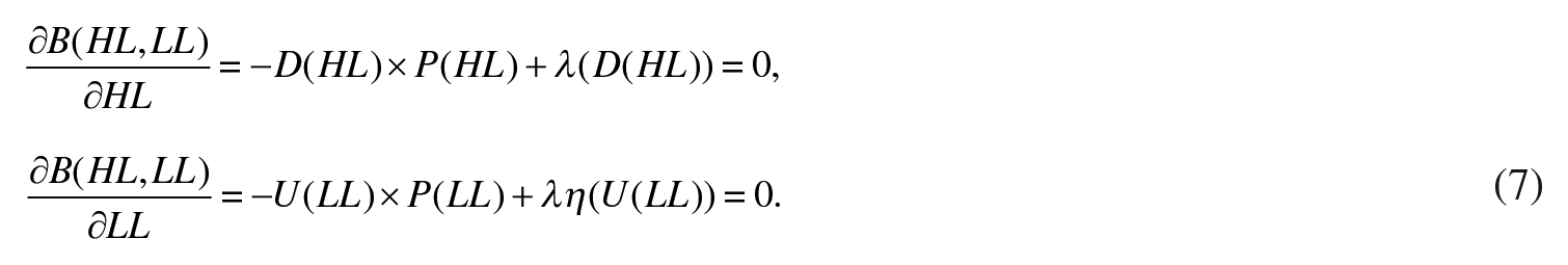
It follows that:

$$\lambda =\mathrm{P}\left(\mathrm{HL}\right)=\frac{P(LL)}{\eta }.$$

(8)

The result in Equation (8) implies that short-run economic efficiency occurs when the high price, P(HL), is just high enough to compensate for the round-trip inefficiency of storage when buying energy at the low price, P(LL). The dashed red line in Figure 2(b) corresponds to P(LL)/η and the short-run optimum corresponds to reducing the peak net-load by nearly 8 GW. However, this result does not account for the capital costs of installing the storage or the savings in the capital cost of the installed generating capacity needed for adequacy. Both of these capital costs must be considered to determine the optimum conditions for long-run efficiency.

The capital cost of storage, KCS(L), is specified to be optimally determined and proportional to the total amount of energy stored, assuming that no there is no spared energy capacity, and given by:

$$KCS\left(LL\right)=KS{\int }_{ML}^{LL}U\left(\mathrm{L}\right)\mathrm{dL}.$$

(9)

In contrast, the savings in the capital cost of installed generating capacity, KCG(PL, HL), is proportional to the reduction of the peak load, and it is given by

$$KCG\left(PL,HL\right)=KG(PL-HL).$$

(10)

Including these two capital costs in the objective function leads to the following optimum relationship between the high and low prices, P(HL) and P(LL):

$$P(HL)=\frac{P(LL)+KS}{\eta }-\frac{KG}{D(HL)}forP(HL)>P(LL).$$

(11)

The results in Eq. (11) show, as expected, that adding the capital cost of storage, KCS, increases the difference between P(HL) and P(LL), and adding the savings in the capital cost of generating capacity, KCG, reduces this difference. If KS / η < KG / D( HL ), then P(HL ) < P(LL)/ η and the incremental cost of supply no longer covers the round-trip inefficiency of storage. However, the optimum P(HL ) > P(LL), and when P(HL) = P(LL) the load profile is flat, corresponding to the maximum amount of usable storage.

The results in Figure 1(b) show the optimum results when the objective is to minimize the total daily operating costs. ⁷ The optimum capacity of storage is 71.13 GWh of deliverable energy, corresponding to 71.13/0.86 = 82.71 GWh of purchased energy, and the peak net-load is reduced from 54.92 GW to 47.43 GW, a reduction of 7.49 GW. The total savings in the cost of energy is $3.598 million, $2.039 million for deferrable load and $1.558 million for non-deferrable load. Even though the hourly purchases for non-deferrable load do not change with storage, the reduction of the peak net-load reduces the price paid during the day when the non-deferrable load is highest. For deferrable load, the savings from shifting load are partially offset by the additional energy purchased off-peak to cover the round-trip inefficiency of storage.

When the cost of installing the storage capacity is added to the objective function, the optimum reduction of the peak load and the amount of storage needed will be lower. The capital cost of storage capacity is determined as the cost per charge/discharge cycle in $/MWh, and the details are given in Lamadrid et al. (2016). Only a summary is presented here. The annualized cost of thermal storage capacity is $12,500/MWh and the annual number of cycles for cooling is 93. Consequently, the capital cost per cycle is $134.41/MWh of energy purchased, which, due to the 86 percent round-trip efficiency of storage, is equivalent to 134.41/0.86 = $156.29/MWh of energy discharged. However, when this cost is added to the objective function, there is no economic justification to install any storage even though the supply curve is relatively inelastic and the peak/off-peak price difference is large. This result is consistent with the conventional view that investing in storage is not economically viable unless some benefits from reducing the peak net-load are realized.

When the savings in the capital cost of installed generating capacity due to reducing the peak net-load are added to the capital cost of storage, the results change radically. The details for deriving this capital cost are also given in Lamadrid et al. (2016). The rationale for the derivation is to allocate the annualized cost of a peaking unit to a specified number of peak-load hours. It is assumed that regulators have specified a target that all generating units should be dispatched for at least 100 hours per year (i.e. capacity factor > 1.14%). Inspection of the annual load duration curve shows that imposing such a requirement would reduce the peak net load by 6 GW from 55 GW to 49 GW, a reduction of over 10 percent. The annualized capital cost of generating capacity is $80,000/ MW, and allocating this amount to 100 hours implies that the capital cost is $800/MW for each peak hour. There are 11 hours with net loads above 49 GW for the day shown in Figure 1(a), and the saving in the capital cost of generating capacity is $8,800/MW reduction of the peak net-load. Adding this saving to the objective function leads to another corner solution. The optimum is to use as much storage capacity as needed to make the daily profile of net-load completely flat.

The optimum peak net-load is now HL = LL = 45.50 GW, corresponding to a reduction of 9.42 GW, and the optimum capacity of storage is 99.61 GWh. The total saving from flattening the load profile is $70.581 million, composed of $3.278 million savings from the cost of energy, -(99.61×156.29/1000) = -$15.568 million for the capital cost of storage, and +(9.42 × 8800/1000) = $82.871 million savings from reducing the peak net-load. If both the cost of storage and the savings from the reduced peak are allocated to the deferrable load, as they should be, the savings are $68.092 million for deferrable load, and only $2.489 million for non-deferrable load.

The general conclusions from this example are important for planning and regulatory purposes. The amount of installed generating capacity needed for system adequacy is determined by the forecast of the annual peak net-load. Hence, the net-savings in capital costs from reducing this peak and installing the storage needed are the main factors determining the long-run economic efficiency, and the high cost of generating capacity is the dominant factor in this example. As a result, it is economically efficient to flatten the load profile and reduce the peak net-load to 45.5 GW, which is well below the specified regulatory target of 49 GW.

The discussion in the next section introduces the uncertainty of wind generation, and it explains how distributed storage can be used to provide ramping services that compete with shifting load from peak to off-peak hours. Since the standard operating criterion for dispatching units is to minimize short-run costs, the size of the peak/off-peak price differential determines the relative importance of ramping versus load shifting. The main focus of the analysis is on situations when the supply curve is relatively elastic and obtaining long-run efficiency on peak-load days requires some form of intervention, such as critical peak pricing.

4. An Economic Assessment of Storage: Stochastic Case

The empirical example in Section 3 demonstrates how the optimal management of distributed storage is affected by considering the capital cost of storage capacity, the savings from reducing the annual peak net-load, and the associated capital costs of generating capacity. When only the operating costs of meeting net-load are minimized, there is an optimal level of storage capacity that determines an peak/off-peak price ratio that is large enough to cover the round-trip inefficiency of the storage. This is consistent with the standard criterion for short-run efficiency used by a system operator. Adding the net-capital costs leads to a corner solution, and long-run efficiency implies increasing the storage capacity to flatten the daily load profile on the peak-load day.

In this section we determine how these results are affected by introducing the uncertainty of wind generation, implying that storage can provide ramping services as well as shift the load. When the peak/off-peak price differential is large enough, the dominant strategy is to use storage to shift load from expensive periods to less expensive periods. However, if the price differential is small, the dominant strategy is to use the storage to provide ramping (e.g., Figure 1.11, CAISO, 2018). If storage is used for ramping services on the annual peak-load day, the outcome will be inefficient from the long run perspective. This latter situation provides the established rationale for using some form of intervention such as Critical Peak Pricing (CPP) (see Section 2).

The first step in the analysis is to determine the optimum bidding strategy for a given amount of distributed storage when there is uncertainty about the future price of purchasing electricity from the wholesale market. We have shown in Lu et al. (2015) that the optimum strategy is to submit bids, based on a stochastic forecast of prices for the next 24 hours, with two price thresholds, a high-price threshold for discharging and a low-price threshold for charging. When there is sufficient storage capacity, the thresholds remain constant throughout the day, and the ratio between them is determined by the round-trip inefficiency of storage. This bidding strategy provides ramping services implicitly because purchases from the grid will increase/decrease if the price is low/high enough. As the price is a function of the net-load, it will be higher/lower when wind generation is lower/higher than expected. We use simulations of different realized levels of wind generation and price to evaluate how different storage strategies perform. For a given amount of storage capacity, the focus is on comparing the realized reductions in the peak net-load and identifying the most effective storage strategy.

The statistical specifications for wind generation and the price are described in Appendix A. The model for wind generation has a daily cycle to represent the mean (it is higher at night) and normally distributed AR[1] residuals. The AR coefficient is large and positive to replicate the observed persistence of wind generation when it is higher/lower than expected. Load is exogenous, and consequently net-load is a stochastic function of wind generation. We specify a linear price function of the net-load plus an IID white-noise residual. Consequently, it is straightforward to derive the mean and variance of the forecasted prices for the next 24 hours given the initial conditions.

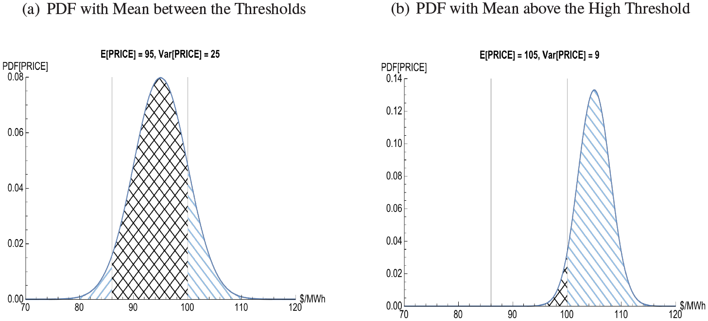
The mean and variance of the price for any given hour determine the probabilities of charging, discharging or doing neither, as the two price thresholds remain constant. Figure 3 illustrates this for two different Probability Density Functions (PDF) of the price. The threshold prices are $100MWh and $86/MWh, implying that the round-trip efficiency of storage is 86%. Figure 3(a) shows a PDF with the mean between the two thresholds and a relatively large variance. The probabilities of charging (4%, when the price < 86)) and discharging (16%, when the price > 100) are small, and it is highly likely (80%, when 86 < price < 100) that the stored energy will remain the same for this hour. This crosshatched area between the price thresholds corresponds to being available for ramping. For example, if the charging and discharging rates are 6 χ 0.86 = 5.16 GW ⁸ and 6 GW, respectively, the expected change in the amount of deliverable energy stored is -0.75 GWh. In contrast, Figure 3(b) shows a PDF with the mean above the high threshold and a relatively small variance. As a result, the probability of discharging (95%) is high, and the corresponding expected change in the stored energy is -5.71 GWh. The implication from Figure 3(a) is that the stored energy is available to provide up-ramping (discharging) or down-ramping (charging) for the grid when the realized price crosses one of the price thresholds. Alternatively, in Figure 3(b), shifting the peak load (purchased energy) down dominates. As we show later, with CPP every hour can be classified as either charging or discharging, and virtually no ramping is provided.

Figure 3:

Two Examples of Charging/Discharging Probabilities*

4.1 Optimal Bidding Strategy for Distributed Storage

We set the objective of an aggregator to manage distributed storage to minimize the expected cost of purchasing energy from the wholesale market, subject to meeting the given energy needs of the customers on a daily basis. Consequently, this is a non-invasive strategy in the sense that the hourly pattern of purchases (load) changes but the hourly pattern of demand (energy used) stays the same. The optimal strategy is to submit bids with price thresholds for charging, P(LL), and discharging, P(HL), energy storage.

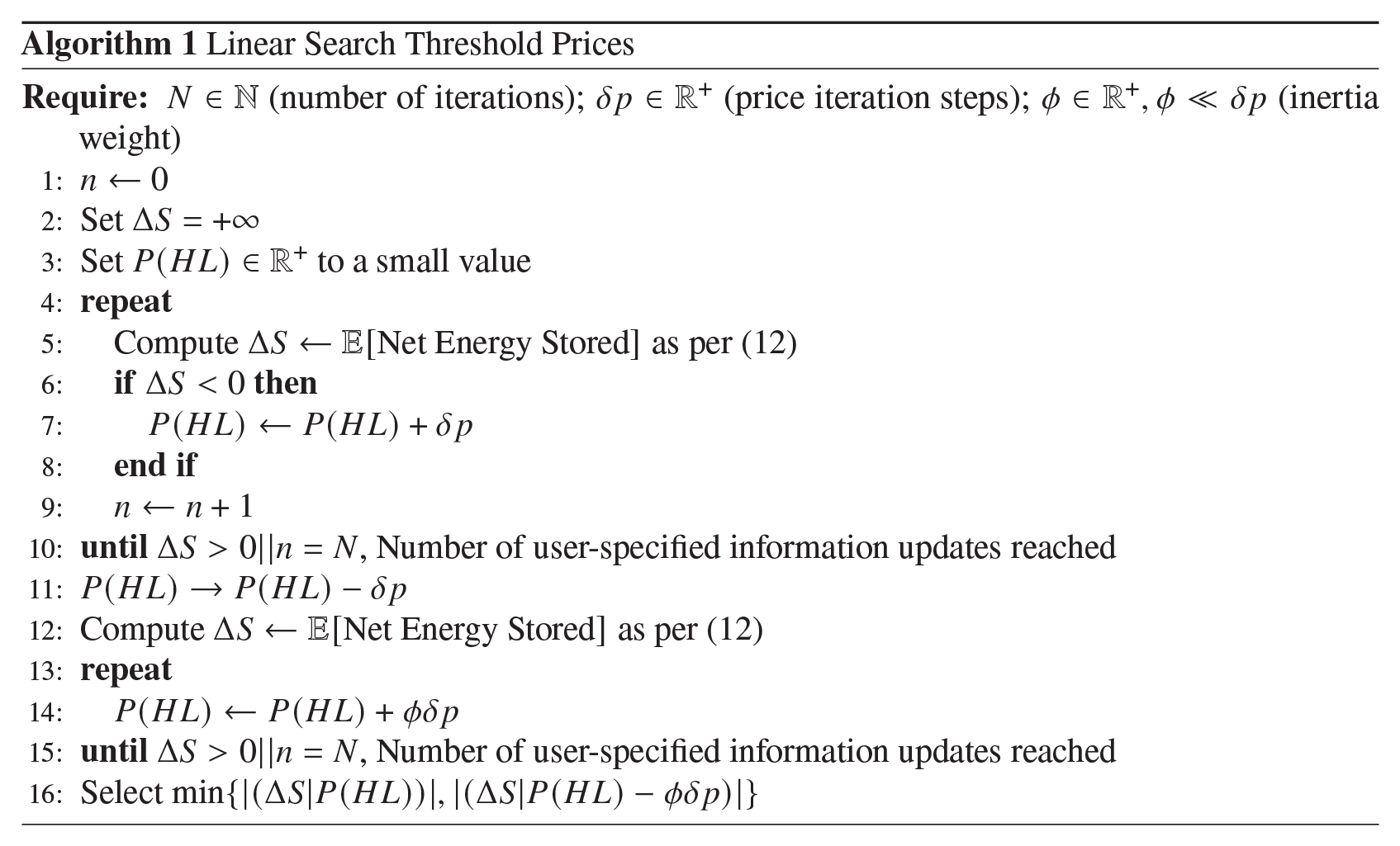
For a given hourly pattern of demand and the corresponding forecast of the wholesale prices, a one-dimensional search is used to determine the optimum high threshold P(HL). ⁹ This corresponds to making the expected amount of energy stored at the end of the horizon equal to the initial level, and hence avoid considering the energy stored as a free source. Using the notation listed in Definition 1, the expected net energy stored at the end of the horizon for a given P(HL) is:

$$\mathbb{E}[NetEnergyStored]=\sum _{t\in T}(\mathbb{P}(\mathbb{E}[P^t]<\eta P(HL))c-\mathbb{P}(\mathbb{E}[P^t]>P(HL))\min \{D^t,d\}).$$

(12)

where Ρ denotes the PDF of a Normal density with known mean and variance for each hour, and c and d are the specified maximum rates of charging and discharging, respectively.

Starting with an initial low value of P(HL), the steps for computing the optimum value are listed in Algorithm 4.1. This corresponds to searching for P(HL) to make the final expected net-energy stored in 12 equal to zero.

Algorithm 1 Linear Search Threshold Prices

Require: Ν ∈ N (number of iterations); δρ ∈ R+ (price iteration steps); φ ∈ R+,φ << δρ (inertia weight) 1: n ← 0 2: Set ΔS = +∞ 3: Set Ρ(HL) ∈ R+ to a small value 4: repeat 5: Compute ΔS ← E[Net Energy Stored] as per (12) 6: if ΔS< 0 then 7: Ρ (HL) ← Ρ (HL)+ δρ 8: end if 9: n ← n + 1 10: until ΔS> 0||n = Ν, Number of user-specified information updates reached 11: Ρ (HL) → Ρ ( HL)- δp 12: Compute ΔS — E [Net Energy Stored] as per (12) 13: repeat 14: Ρ (HL) ← Ρ ( HL)+ φδρ 15: until ΔS> 0||n = Ν, Number of user-specified information updates reached 16: Select min{|(ΔS|P(HL))|, |(ΔS|P( HL)-φδρ)|}

4.2 Comparing the Performance of the Bidding Strategy for Inelastic and Elastic Supply

In this section we determine how well the bidding strategy with price thresholds, described in the previous section, performs for two different supply curves. Both curves use a stochastic form of the linear function in 4. One has an inelastic supply, with a slope of 4, and the other has an elastic supply, with a slope of 0.4. A complete description of the stochastic characteristics of these two supply curves is given in Appendix A.

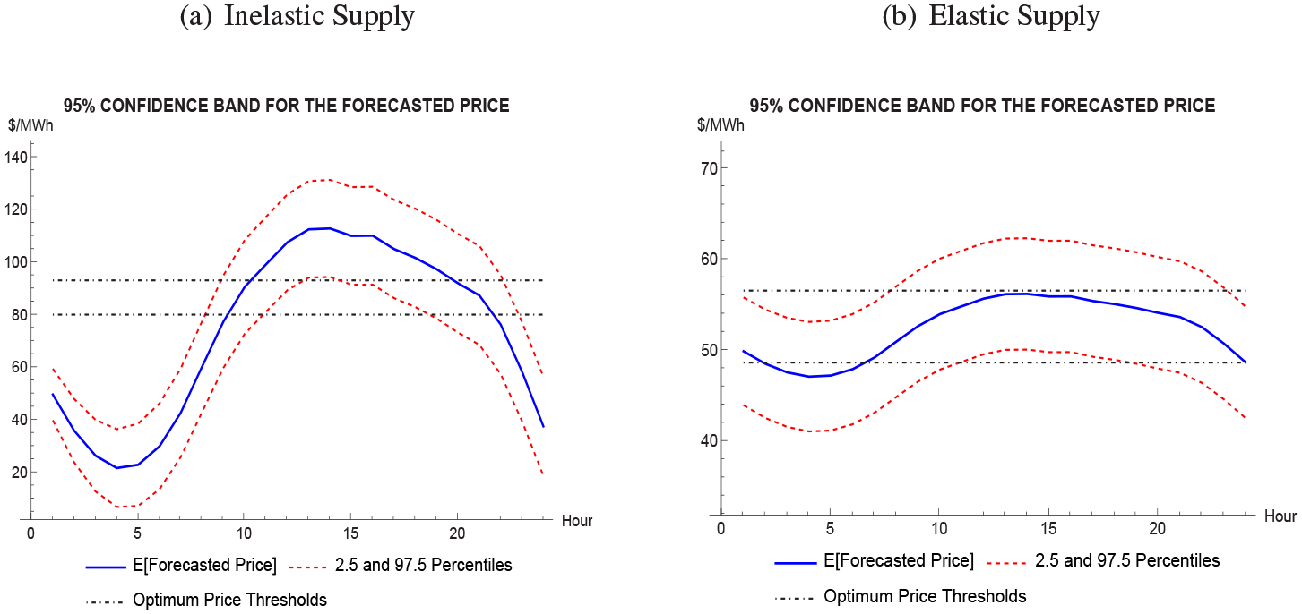
Using the levels of net-load presented in Figure 1(a), confidence bands for the forecasted price are shown for the two supply curves in Figure 4. Note that the vertical scales are not the same, and the variances and the range of hourly E[price] are much larger for inelastic supply. The two horizontal lines correspond to the high and low price thresholds, and for the inelastic supply in Figure 4(a), they are 93.30 and 80.24 $/MWh, and for the elastic supply in Figure 4(b), they are 56.67 and 48.74 $/MWh. The important difference between these two forecasts is that the confidence band for inelastic supply falls mostly above or below the thresholds, but for elastic supply, it falls mostly between the thresholds. Consequently, the dominant strategy when the supply is inelastic is to charge storage at night and discharge it during he day. In contrast, ramping (neither charging or discharging) is dominant when the supply is elastic. This conclusion is confirmed in Figure 5 which shows the hourly cumulative probabilities for charging, ramping (crosshatched area) and discharging storage for the two supply curves. The numerical values of the probabilities shown in Figure 5 are summarized in Table 1.

Figure 4:

Confidence Bands for the Forecasted Price of Energy

Figure 5:

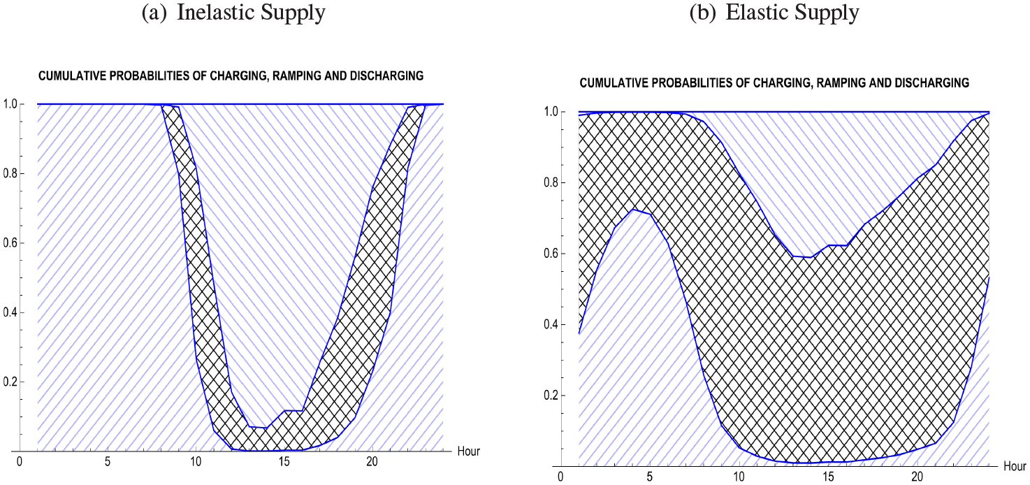
Hourly Cumulative Probabilities for Charging, Ramping and Discharging Storage*

Table 1:

Average Hourly Probabilities of Charging and Discharging Storage

Storage Strategy	Supply	Charging	Discharging	Ramping a
Price Thresholds	Inelastic	0.49	0.38	0.13
Price Thresholds	Elastic	0.22	0.18	0.60
Price Thresholds + CPP*	Elastic	0.46	0.38	0.16

a

Ramping represents the probability that storage is neither charged nor discharged.

The probabilities shown in Figure 5 for inelastic and elastic supply affect the expected amount of energy stored. Given the price thresholds and the initial level of stored energy, the expected amount of deliverable energy stored at the end of Hour t is:

$$\mathbb{E}[S^t]=S^{t-1}+\mathbb{P}\left(\mathbb{E}\left[P^t\right]<\eta P\left(HL\right)\right)\mathrm{c}-\mathbb{P}\left(\mathbb{E}\left[P^t\right]>P\left(HL\right)\right)min\{D^t,\mathrm{d}\},\forall \mathrm{t}\in \mathrm{T}.$$

(13)

For this analysis, we assume that the capacity of storage is 70 GWh, which is similar to the optimum amount for short-run efficiency in Section 3. The maximum rates of charging and discharging are both set to 6 GW, implying that fully charging storage would take nearly 12 hours. ¹⁰ Given the initial level of deliverable energy stored of 25 GWh, the expected hourly levels of deliverable energy stored are shown in Figure 6. For inelastic supply, the minimum energy stored is 14 GWh with a maximum of 68 GWh (range = 54 GWh). In contrast, the corresponding values for elastic supply are a minimum of 21 GWh and a maximum of 46 GWh (range = 25 GWh). In other words, twice as much load is shifted on average when the supply is inelastic.

Figure 6:

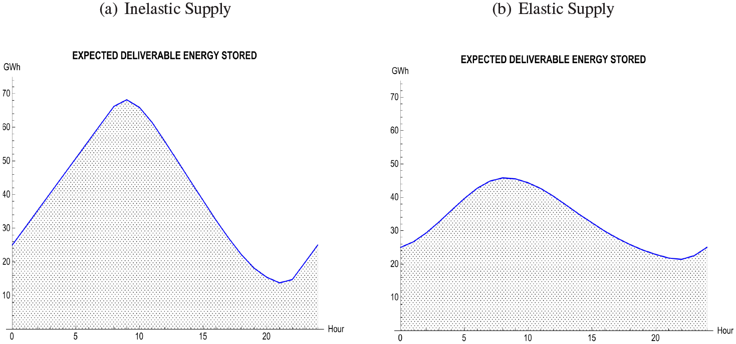
The Expected Hourly Levels of Deliverable Energy Stored

The overall effects of shifting the load on the two supply curves are shown in Figure 7, and the corresponding reductions of the expected peak net-load are summarized in Table 2. ¹¹ The expected reduction is 5.89GW for inelastic supply, but it is only 2.64 GW for elastic supply. ¹² The new peak of 49.03 GW with inelastic supply is essentially equal to the regulators' target peak of 49 GW, but with elastic supply, the new peak (52.28 GW) is 3.25 GW higher. Since the results in Section 3 show that long-run efficiency corresponds to a flat daily net-load profile, a larger peak reduction is more efficient. Consequently, the analysis now considers how to accomplish this when the supply is elastic, and specifically, how well CPP with elastic supply performs.

Figure 7:

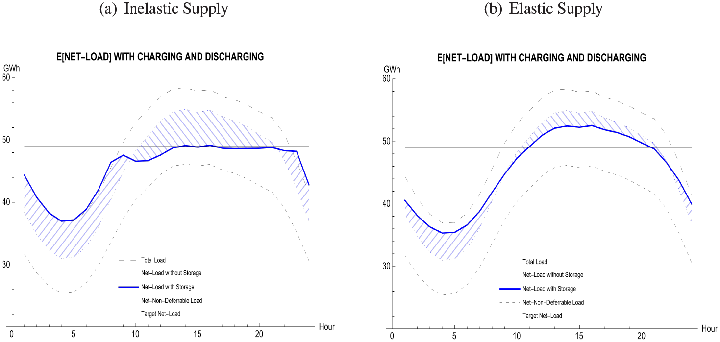
The Effect of Distributed Storage on the E[Hourly Net-Load]

Table 2:

Simulated Reductions in the Peak Net-Load with Storage (GW)

	Supply	Forecasted	Simulated	Simulated	Simulated
Storage Strategy	Curve	Reduction	Mean	Minimum	5th Percentile
Price Thresholds	Inelastic	5.89	5.84	1.32	2.64
Price Thresholds	Elastic	2.64	2.46	-3.48	-2.79
Price Thresholds + CPP	Elastic	5.92	5.46	-3.48	1.12
Price Thresholds + CPP*	Elastic	5.03	5.06	0.90	1.68
Robust Heuristic	Elastic	5.92	5.11	2.52	2.66

4.3 The Requirements for Maintaining System Adequacy

The reductions of the expected peak net-load shown in Table 2 confirm the standard conclusion in the literature that a small reduction of the peak net-load when the supply is elastic is very inefficient from a long-run perspective. However with stochastic wind generation, this metric can be a misleading way to determine the requirements for generation adequacy. Our proposed alternative does not change the general conclusion about elastic supply, but it does set a more stringent standard for adequacy.

The established reliability standard adopted by the North American Electric Reliability Corporation (NERC) is that the bulk-power grid should only fail on average one day in ten years. This corresponds to a failure rate of < 0.001%, and for our analysis, we approximate this by considering the worst case with the lowest realized wind generation in 1000 simulated realizations of the peak-load day. The procedure adopted by the NERC in the annual Long-Term Reliability Assessment is to use forecasts of the annual peak loads ten-year ahead for different regions to ensure that each region has enough installed generating capacity to meet these forecasted peaks. The definition of "enough" is specified to be the forecasted peak load plus a specified reserve margin. The main responsibility for confirming that this criterion actually does meet the reliability standard rests on the state-level public service commissions, and for each region, simulations of various equipment failures (contingencies) are evaluated to ensure that the installed generation capacity can meet the forecasted peak loads and cover the contingencies. This was a viable procedure when the future peak loads could be forecasted accurately, but now with higher penetrations of renewable generation, there is a lot more uncertainty forecasting future peak net-loads.

In addition, there is an important difference between the uncertainty of contingencies and the uncertainty of wind generation. ¹³ Individual equipment failures are relatively rare events, but the variability of wind generation occurs every-day. Consequently, we argue that this latter source of uncertainty should be incorporated into setting the initial requirements for generation adequacy. Our proposal is to use the forecasted peak net-load plus the up-ramping capacity needed to replace the forecasted peak net-load as the criterion. The basic rationale for this change is that the capabilities of the system, such as the amount of available storage capacity, can modify the amount of up-ramping needed to maintain operating reliability and the amount of generating capacity needed for adequacy. In other words, to meet the standards for adequacy, there must be enough conventional generating capacity installed to meet both the peak net-load and cover the uncertainty of wind generation. We now demonstrate why using the expected peak reduction as the criterion for adequacy can exaggerate the size of the attainable reduction of the peak net-load.

The new results are based on 1000 stochastic simulations to determine how well the different storage strategies perform for the "worst" case, corresponding to the case with the highest net-load. The different daily realizations of wind generation and the price of electricity are generated using the stochastic models for wind generation and price described in Appendix A. The initial conditions for generating hourly realizations of wind generation require specifying values for u₀ and e₀, and these are 1.5 × σ _e =1.5 and 0, respectively. The other parameter values are shown in Definition 3. The random residuals for wind generation, e^t, and price, v^t, are generated separately using two different seeds to ensure that exactly the same realizations are used to evaluate each storage strategy. Since the optimum price thresholds are based on the forecasted hourly prices, the thresholds remain the same for all of the simulated realizations for each strategy.

Each realization of wind generation determines the net-load and, with the addition of the random residual v^t, the corresponding price. This realized price determines how the storage is actually used. Even though the optimal bidding strategy restricts the expected amount of energy stored in Hour 24 to equal the initial amount in Hour 0, this restriction does not apply to individual realizations. As a result, it is important to enforce the capacity limits of storage and the and maximum charge and discharge rates for each realization. Since the auto-correlation of wind generation is large and positive (ρ = 0.9), deviations from the forecasted values tend to be persistent, and it is highly likely that the stored energy will reach 0 or the maximum capacity (70 GWh) before Hour 24. In fact, running out of stored energy before the end of a peak period is one way to seriously undermine the performance of a storage strategy.

The results for four different storage strategies are based on the same sample of 1000 realizations, and the simulated reductions in the peak net-load are summarized in Table 2. The first two rows correspond to the inelastic and elastic supply, and the other two rows represent new strategies that will be discussed later in Sections 4.4 and 4.5. Note that all peak reductions are computed as the difference from the forecasted peak before storage (54.92 GW) to ensure that all the reductions in Table 2 are comparable. For example, the Simulated Mean reduction is defined as:

$$\mathrm{Simulated}\mathrm{Mean}\mathrm{Reduction}=54.92-\mathrm{Average}\mathrm{Simulated}\mathrm{Daily}\mathrm{Peak}\mathrm{with}\mathrm{Storage},$$

(14)

The values of the simulated mean reductions are similar to the corresponding forecasted reductions, but the minimum reductions, representing the worst case with unexpectedly low wind generation are lower. Nevertheless, these minimum reductions are better metrics for generation adequacy.

The minimum reduction is substantially smaller (1.32 GW) than the forecasted reduction (5.89 GW) for inelastic supply (Row 1), and it is negative (-3.48 GW) for elastic supply (Row 2). Even if some of the worst realizations are ignored by using the 5th percentile reduction, the minimum reduction for elastic supply is still negative. Hence, a better strategy is needed to increase the size of the peak reductions and still meet the standards for generation adequacy when the supply is elastic.

Before introducing the definition of an"attainable" peak reduction, it is helpful to determine the trade-off between peak reductions and the amount of storage capacity needed to ensure that adequacy standards are met. Figure 8(a) shows a histogram of the simulated daily amounts of energy discharged to meet the regulatory target load of 49 GW. ¹⁴ The range of possible daily values is large, with a minimum of 0.5 GWh (dotted line) and a maximum of 86.8 GWh (solid line). Given the initial information available at t = 0, it follows that covering all of these simulated possibilities requires that at least 86.8 GWh of storage capacity is available, even though the average capacity used is only 44.7 GWh (dashed line). The large range of values illustrates the effects of persistence on the realized levels of wind generation. If the realized levels are higher/lower than the expected levels, the forecasting errors tend to accumulate into large negative/positive deviations from the mean, and these deviations represent the down/up ramping needed to mitigate the variability of wind generation.

Figure 8:

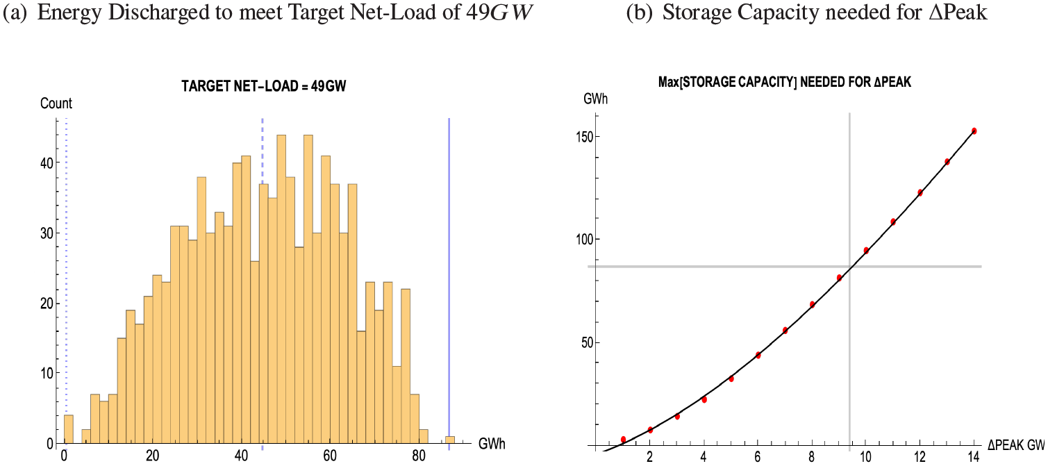
The Trade-off between Peak Reductions and Storage Capacity

The maximum discharge of 86.8 GWh provides the maximum up-ramping needed to ensure that the peak load < 49 GW for all realizations, and consequently, it meets the reliability standard for generation adequacy. These results illustrate why meeting this standard is so challenging.

Nevertheless, the potential savings in capital costs from reducing the peak net-load are substantial and should not be overlooked. Figure 8(b) shows the locus of the maximum storage capacity needed for a range of reductions from the maximum simulated peak net-load (58.4 GW). ¹⁵ The solid grid lines correspond to the example in Figure 8(a) with the target load equal to 49 GW (ΔPeak = 58.4 -49 = 9.4 GW) and the storage capacity equal to 86.8 GWh. The simulated values of the maximum storage capacity in Figure 8(b) (dots) were fitted to a cubic function of the peak reduction, and the fit was very good with an R² of 99.99%. The derivative of this function corresponds to Figure 2(a) for the deterministic case, and it is used to compute the trade-off between the peak reduction and the incremental amount of storage capacity needed for adequacy.

It is possible to derive the optimal conditions for storage capacity that are similar in form to Equation 11 in Section 3 for the deterministic case. The trade-off shown in Figure 8(b) corresponds to the trade-off between storage capacity and the peak reduction in Figure 2(a). The main differences in the optimum conditions for stochastic net-load compared to deterministic net-load are (1) the savings in energy purchases are now based on the average simulated net-load rather than the forecasted net-load, and (2) the trade-off between storage capacity and the peak reductions is the locus shown in Figure 8(b) rather than the reductions shown in Figure 2. Nevertheless, the basic structure of the objective function remains the same. The optimum relationship between the high price and the low price of energy shown in Equation 8 is identical. Hence, the distinguishing feature of the optimization for stochastic net-load is how the capital costs are represented. The optimum condition for the deterministic case in Equation 11 can be rewritten for the stochastic case as follows:

$$P(HL)=\frac{P(LL)}{\eta }+\frac{KS}{\eta }-\frac{KG}{D2(HL)}forP(HL)\ge P(LL)$$

(15)

Where

P(HL) is the energy price at the high net-load, HL, $/MWh.

P(LL) is the energy price at the low net-load, LL, $/MWh.

KS is the capital cost of storage, $/MWh.

KG is the capital cost of generating capacity, $/MW.

D2(HL) is the incremental storage capacity needed, GWh/GW.

η is the round-trip efficiency of storage, %/100.

In Equation 15, D2(HL) is the derivative of the locus shown in Figure 8(b), and it replaces D(HL) in Equation 11. D2(HL) covers the worst realization with the lowest wind generation and the highest up-ramping. In contrast, D(HL) corresponds to the locus between the mean storage capacity and the peak reduction. The deterministic optimum in Equation 11 is a special case of the stochastic optimum in Equation 15 when no up-ramping is needed and D2(HL) = D(HL). This corresponds to having perfect forecasts of wind generation. There would be no surprises, the forecasted peak reduction would be realized, and the storage capacity needed for attainability would be the same as the forecasted amount. Even though the deterministic case represents an extreme situation, reducing the amount of up-ramping needed by, for example, using more accurate forecasts of wind generation is always an effective way to increase the attainable peak reduction for a given amount of storage capacity. In spite of the extra storage capacity needed to meet adequacy standards, the results shown in Section 4.5 still confirm the conclusions in Section 3. It is efficient in the long-run to use as much deferrable demand as feasible until the net-load profile is perfectly flat.

Appendix B presents a simple example to introduce the concept of an "attainable" peak reduction that is a reliable metric for determining generation adequacy. To be compatible with our convention for peak reductions in Table 2, the attainable peak reductions are measured from the forecasted peak (54.92 GW) rather than the maximum simulated peak (58.4 GW). Appendix B also shows why the mean reductions in Table 2 can be larger than the attainable reductions. From this point on, the maximum discharge rate is enforced, and the term ΔPeak is used to represent an attainable peak reduction that follows the conventions in Table 2. The definitions of the attainable and mean reductions are:

$$\Delta \mathrm{Peak}\le \left(\mathrm{Max}\left[\mathrm{Discharge}\mathrm{Rage}\right]-\mathrm{Up}-\mathrm{Ramping}\mathrm{at}\mathrm{the}\mathrm{New}\mathrm{Peak}\right),$$

(16)

$$\mathrm{Mean}\mathrm{Reduction}\le \mathrm{Max}\left[\mathrm{Discharge}\mathrm{Rate}\right],$$

(17)

The corresponding up-ramping needed is: ¹⁶

$$\mathrm{Up}-\mathrm{Ramping}\mathrm{Needed}=\mathrm{Max}\left[\mathrm{Simulated}\mathrm{Net}-\mathrm{Load}\right]-\mathrm{Forecasted}\mathrm{Peak}\mathrm{Net}-\mathrm{Load},$$

(18)

4.4 The Limitations of Critical Peak Pricing

The economic predicament illustrated by the results for elastic supply in Table 2 is that there is no guarantee that the diurnal price differentials on peak-load days will be large enough to make shifting load the dominant strategy for storage. Therefore, storage will be used inefficiently with elastic supply from a long-run perspective. This problem is likely to be exacerbated given the current replacement of coal-fired and nuclear units by natural gas units (see EIA (2019)). For the next few years in the northeastern states, natural gas will be dispatched throughout the day and may set the wholesale price all day. For this reason, there is a clear economic justification for evaluating Critical Peak Pricing (CPP) as a possible way to provide the incentives needed to improve the long-run efficiency of storage.

The savings in capital costs from reducing the peak net-load presented in Section 3 are $800/MW. Adding this amount to the energy price for a specified number of peak hours would definitely provide incentives for shifting load, but it is unnecessary to impose such extreme measures. Using a surcharge of only $80/MWh is large enough to replicate the price differences shown in Figure 4(a). ¹⁷ The effect of CPP on the hourly prices is shown in Figure 9(a). The surcharge of $80/ MWh is added from 11:00 to 21:00 to the price profile shown in Figure 4(b). This CPP period corresponds to the hours when the forecasted net-load is greater than the regulatory target of 49 GW. ¹⁸

Figure 9:

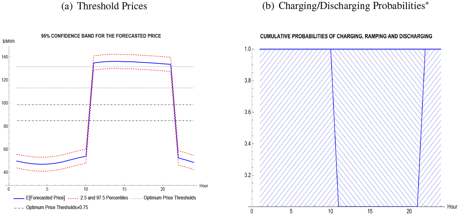
The Threshold Prices and Charging/Discharging Probabilities for the CPP* Strategy

Two sets of price thresholds are shown in Figure 9(a). The two highest thresholds (dotted) corresponds to the optimum thresholds derived using Algorithm 1. It is clear, however, that the high threshold (131.75 $/MWh) falls in the 95% confidence band for the price during the peak period, and this causes problems. The variability of the price results in some realized prices below the high threshold during the peak period. When this happens, the price signal is to not discharge storage, and the net-load has to be met entirely by purchases from the grid. Even though the simulated average peak reduction with CPP (5.46 GW) is relatively large, the minimum reduction is still negative (-3.48 GW). This is exactly the same value as the minimum for Elastic Supply in Table 2, ¹⁹ and therefore, there is no improvement for adequacy purposes from using this direct application of CPP.

The performance of CPP can be improved for adequacy purposes by making some simple modifications to the storage strategy. The first one is to lower the price thresholds so that the high threshold is well below the realized prices during the peak period. The new thresholds in Figure 9(a) (dot/dashed) are 0.75 times the original thresholds. ²⁰ This change maintains the ratio between the low and high thresholds, and more importantly, it avoids having realized prices below the high threshold during the peak period. The two modified thresholds are $98.81/MWh and $84.98/MWh. Using these new thresholds, the cumulative probabilities for charging and discharging are shown in Figure 9(b). The implication is that the new thresholds discriminate perfectly between charging and discharging, and the probability of ramping is always zero. ²¹ In addition, the hourly discharge rate is calibrated to ensure that discharging can occur for all 11 hours of the peak period.

There is one additional modification that is made to limit the amount of ramping caused by storage at the beginning and end of the peak period. Using the probabilities in Figure 9(b), storage would switch from charging to discharging in Hour 11 and from discharging to charging in Hour 22. In both cases, this would imply changing the load by (Charge Rate + Discharge Rate) which could be as high as 12 GW. To avoid these sudden changes in the load, the amount of stored energy is held constant in Hour 10 and Hour 22. This implies that discharging occurs for all hours with a surcharge, but charging is delayed by one hour at each end of the peak period. Without this modification, the realized peaks generally occur in Hours 10 or 22. This modified CPP strategy is referred to as Elastic Supply + CPP* in Table 2, and in the text from this point on.

In spite of the modifications made to improve the performance of the CPP strategy, the results in Table 2 for CPP* are still disappointing. The simulated mean reduction of 5.06 GW looks promising, but the minimum reduction of only 0.90 GW is the metric that matters for generation adequacy. CPP* is always vulnerable to having a high realized net-load occur outside the peak period, and the highest net-load actually occurs in Hour 9 of Realization 561 before the CPP period begins. The underlying problem with CPP* is that the price signals are only minimally sensitive to the realized wind generation, and the storage is discharged throughout the peak period regardless of the realized wind conditions.

Clearly, it would be technically possible to replicate the price behavior for inelastic supply, but we assume that this would not be acceptable to regulators. Hence, the focus now moves to determining how a given amount of distributed storage can be managed to maximize the attainable peak reduction ΔPeak.

4.5 A Robust Way to Reduce the Attainable Peak Net-Load

Although there are many additional modifications to the CPP strategy that could be evaluated, we have chosen to present an alternative heuristic strategy that is sensitive to wind generation rather than the energy price. This strategy is "robust" in the sense that stored energy is discharged only when the realized net-load is above a specified target level. The level of this target depends on the maximum discharge rate and the amount of storage capacity available. If the target net-load is set too low, all of the stored energy will be discharged before the end of the horizon even though realized net-loads higher than the target may still occur. This problem is illustrated in Figure 10(b).

Figure 10:

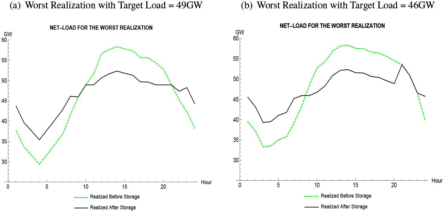
The Net-Load for the Robust Heuristic Strategy on the Worst Realized Day

Figure 10 shows the worst-case net-loads using two different target net-loads. When the target is 49 GW in Figure 10(a), the peak of 52.40 GW occurs in Hour 14 of Realization 988, and this corresponds to the simulated minimum reduction of 2.52 GW for the Robust Heuristic shown in Table 2 (54.92 - 52.40 = 2.52 GW). If the target is set too low at 46 GW in Figure 10(b), the peak of 53.60 GW is higher and occurs later in the day (Hour 21 of Realization 797). The reason for this higher peak is that trying to reach a lower target uses all of the stored energy before Hour 21, and consequently, the net-load in this hour is the same as it is without storage. The corresponding peak reduction is only 1.32 GW (54.92 - 53.60 = 1.32 GW). Consequently, it is important to establish a procedure for determining a target net-load for the robust strategy that avoids the problem exhibited in Figure 10(b).

The procedure for determining the hourly discharge rate for CPP* is discussed first so that it can be compared with the discharge rate for the robust strategy. Using CPP*, the price signal is to discharge for every hour in the peak period. There is no signal to determine how much to discharge each hour. Consequently, to ensure that the stored energy does not run out before the end of the peak period, the hourly discharge for CPP* must obey the following relationship.

$$\mathrm{Hourly}\mathrm{Discharge}\mathrm{Rate}\le \frac{\mathrm{Storage}\mathrm{Capacity}}{\mathrm{Number}\mathrm{of}\mathrm{Peak}\mathrm{Hours}}$$

(19)

All of the results presented in Table 2 are based on identical specifications for storage. The available storage capacity is set at 70 GWh, and the maximum charge/discharge rates are both 6 GW. Since the CPP prices are enforced for 11 hours, the Hourly Discharge Rate for CPP* < 70/11 = 6.36 GW. This implies that the maximum discharge rate of 6 GW, that includes the up-ramping required, can be maintained throughout the peak period using CPP*.

The main difference between CPP* and the robust strategy is that the discharge rate using CPP* is the same (6 GW) for every peak hour, but with the robust strategy, the amount discharged varies. When (Realized Net Load > Target Net Load), Energy Discharged = (Realized Net Load -Target Net Load) ≤ 6 GW for the robust strategy. This procedure holds for all hours of the day, and it can be summarized as follows:

$$\mathrm{Discharge}=\mathrm{Min}\left[\mathrm{Max}\right[\mathrm{Discharge}\mathrm{Rate}\left],\mathrm{Max}\right[\left(\mathrm{Realized}\mathrm{Net}-\mathrm{Load}-\mathrm{Target}\mathrm{Net}-\mathrm{Load}\right),0]]$$

(20)

Given the storage capacity of 70 GWh (dashed), the relationship in Figure 8(b) determines the Peak Reduction = 8.17 GW (dotted), that includes the up-ramping required. This is much larger than the maximum discharge rate of 6 GW, and in fact, Figure 8(b) shows that a target reduction of 6 GW (dashed) only requires 44.34 GW (dotted) of storage capacity to be robust. ²² The conclusion is that the robust strategy would be more effective if the maximum discharge rate was larger, and currently, its performance is handicapped by the limit placed on the discharge rate. In spite of this handicap, the robust strategy still outperforms CPP* in Table 2 even though major adjustments were made to improve the performance of CPP*,

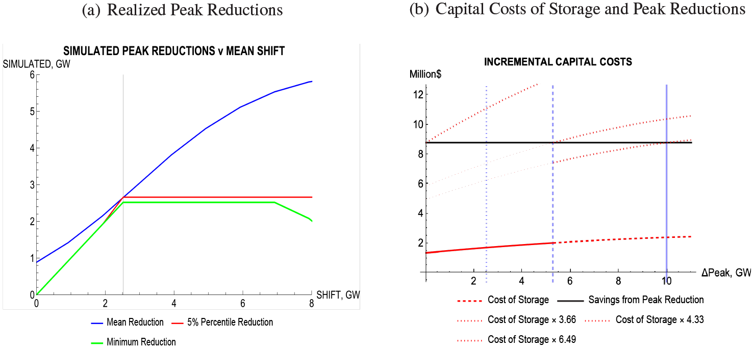
The results in Table 2 show that the simulated minimum reductions of the peak (i.e., ΔPeak with the required up-ramping subtracted) for the CPP* and Robust Heuristic strategies are 0.90 GW and 2.52 GW, respectively. Since ΔPeak for the Robust Heuristic is 2.8 times bigger, this strategy clearly performs best for reducing the generating capacity needed for adequacy. Nevertheless, this peak reduction of 2.52 GW is less than half of the maximum discharge rate of 6 GW, and as a result, it is important to understand why 2.52 GW is the Max[ΔPeak] given the limit on discharging. In Figure 11(a), additional simulations are conducted for the robust strategy to show the trade-off between the target peak reductions and the realized peak reductions.

Figure 11:

Realized Peak Reductions and Capital Costs

In Figure 11(a), a target reduction of the peak net-load is defined as follows:

$$\mathrm{Target}\mathrm{Reduction}=\left(\mathrm{Forecasted}\mathrm{Peak}-\mathrm{Target}\mathrm{Net}-\mathrm{Load}\right)=\left(54.\mathrm{92}-\mathrm{Target}\mathrm{Net}-\mathrm{load}\right)$$

(21)

Consequently, the realized reductions follow the same metrics used in Table 2 and Figure 16 in Appendix B. The largest attainable reduction of the peak (green plot) is Max[ΔPeak] = 2.52 GW. When the target reduction is > 2.52 GW, the realized mean reduction continues to increase but the attainable reduction remains constant at 2.52 GW. When the target reduction is > 7 GW, the attainable reduction falls because the stored energy runs out, just like the example in Figure 8(b). The large range of values with the minimum reduction = 2.52 GW reflects the fact that there is more storage capacity than needed to be efficient. Overall, Figure 11(a) confirms the results for the simple example shown in Appendix B. The main conclusion is that using the mean peak reduction as a metric for adequacy is likely to exaggerate the size of the attainable reduction.

With enough storage capacity, the peak net-load can be reduced until the daily profile of net-load becomes flat, and this puts a hard limit on the size of ΔPeak. In our simulations, the amount of deferrable thermal load is also limiting. The relevant values of net-load and the limits on ΔPeak are:

Max[Total Load] = 58.40 GW

Max[Simulated Net-Load] = 58.40 GW

Max[Forecasted Net-Load] = 54.92 GW

Up-Ramping at Peak = 3.48 GW

Flat Forecasted Net-Load = 44.92 GW

Max[ΔPeak, All Storage] = 10.00 GW

Max[Non-Deferrable Load] = 49.64 GW

Max[ΔPeak, Thermal Storage] = 5.28 GW

In the simulations, the Max[Simulated Net-Load without Storage] = Max[Observed Total Load without Storage] = 58.40 GW because wind generation is zero for the peak hour.

Using the capital cost values derived in Section 3 and the optimum condition in Equation 15 for the stochastic case, the weighted capital cost of storage, KS 77, converts the cost in terms of energy purchased to deliverable energy ($156.29IMWh = $0.15629 millionIGWh for thermal storage). The capital saved from reducing the peak net-load is KG = $8,800IMW = $8.8 millionIGW, and the function D2(HL) in Figure 8 determines how many GWh of stored deliverable energy are needed for a one GW reduction of the peak. For a given ΔPeak, the total capital savings and costs are:

$$\mathrm{Total}\mathrm{Capital}\mathrm{Savings}\mathrm{from}\Delta \mathrm{Peak}=\Delta \mathrm{Peak}\times 8.8\mathrm{million}\$$$

(22)

$$\mathrm{Total}\mathrm{Capital}\mathrm{Cost}\mathrm{of}\mathrm{Storage}=\mathrm{D2}\left(\Delta \mathrm{Peak}\right)\times 0.15629\mathrm{million}\$$$

(23)

It follows that the net-savings in capital costs can be written:

$$\mathrm{Net}-\mathrm{Savings}=(\Delta \mathrm{Peak}\times 8.8-D2\left(\Delta \mathrm{Peak}\right)\times 0.15629\mathrm{million}\$$$

(24)

The First Order Condition (FOC) for maximizing Equation 24 requires taking its derivative and setting it to zero. Figure 11(b) shows the incremental capital savings and costs derived from the locus for D2(HL) in Figure 8(b). ²³ The incremental savings from ΔPeak is simply 8.8, and the incremental cost of storage is the derivative of D2(ΔPeak) × 0.15629. ²⁴

The three grid lines in Figure 11(b) show the Max[ΔPeak] = 2.52 GW for the example with a target net-load of 49 GW presented in Figure 8(a) (dotted), the maximum reduction using all deferrable demand = 5.28 GW (dashed), and the reduction needed to make the net-load profile flat = 10 GW (solid). It is clear from Figure 11(b) that the incremental net-savings in capital costs are still positive when all deferrable demand is used and ΔPeak = 5.28 GW. Further reductions would require an additional form of storage that is likely to be more expensive. If the cost of new storage is less than 3.66 times as expensive as deferrable demand, it is long-run efficient to add enough storage capacity to flatten the net-load profile at ΔPeak = 10 GW. However, if it is more than 4.33 times as expensive, it is not economic to add any additional storage. Finally, if the cost is more than 6.49 time as expensive, it is too expensive to install any storage when there is no deferrable demand available. ²⁵

The overall conclusion is that using the robust strategy with thermal storage is an efficient way to provide attainable reductions of the annual peak net-load and cover the up-ramping required for adequacy. Even with the limit on the rate of discharging, none of the other strategies do nearly as well as the robust strategy for reducing the peak net-load for adequacy purposes.

The district cooling system in downtown Austin, Texas is a good example of a successful thermal storage facility. ²⁶ Water is chilled at night using inexpensive "surplus" wind power, and the cold water is circulated through downtown buildings during the day. ²⁷ Consequently, the buildings on this system do not need air conditioners. Shifting most of the electricity purchased to meet the demand for space cooling from day to night has a major beneficial effect by making the daily net-load profile flatter. With high penetrations of wind generation in the future, periods with surplus wind generation will become more common. The owners of all types of storage could benefit from charging storage when the marginal cost of supply is close to zero and discharging when it is higher. Nevertheless, for customers to reap these benefits, regulators must allow the retail prices paid by customers with storage, as well as the wholesale prices paid, to reflect the real-time marginal costs of supply.

4.6 The Financial Risk of Meeting Adequacy Standards

In Section 4.3, the results in Table 2 show that the size of the attainable reduction (Simulated Minimum) of the peak net-load is substantially larger using the Robust strategy than the CPP* strategy. Incorporating the high capital cost of generating capacity compared to the cost of thermal storage, Figure 11 implies that the Robust strategy is more efficient from a long-run perspective, and total system costs would be lower. Nevertheless, the discussion in this section explains why the owners of distributed storage are likely to prefer the CPP* strategy because it results in higher and more stable savings in the wholesale market.

The CPP* strategy is determined entirely by the price signal to charge or discharge storage, and there is no ramping provided. In our example, the peak realized net-load occurs outside the high-price period when the price signal is to charge storage. In contrast, the robust heuristic strategy ignores price signals and responds only to the realized net-load. Storage is discharged to keep high net-loads as close to the target net-load as possible. With CPP*, storage is fully discharged by the end of the high-price period for every daily realization, but with the robust strategy, storage is only discharged when it is needed to meet the target net-load (49 GW). As a result, the CPP* strategy stabilizes the realized daily savings in the cost of energy purchases, and the Robust strategy stabilizes the realized peak net-load.

The different effects of the two storage strategies are illustrated in Figures 12 and 13, and the corresponding descriptive statistics are summarized in Table 3. The savings in the cost of purchasing energy from the grid in Figure 12 are dramatically different for the two storage strategies.

Figure 12:

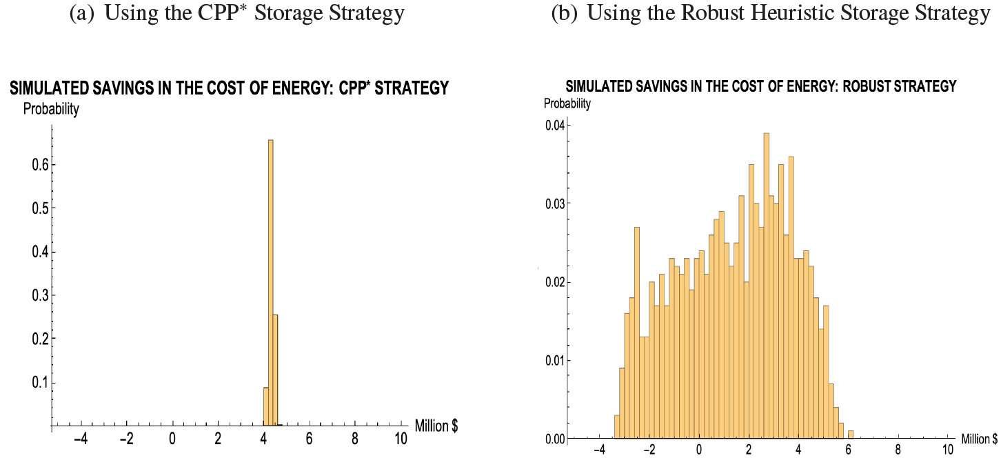
The Simulated Daily Savings in the Cost of the Energy Purchased

Figure 13:

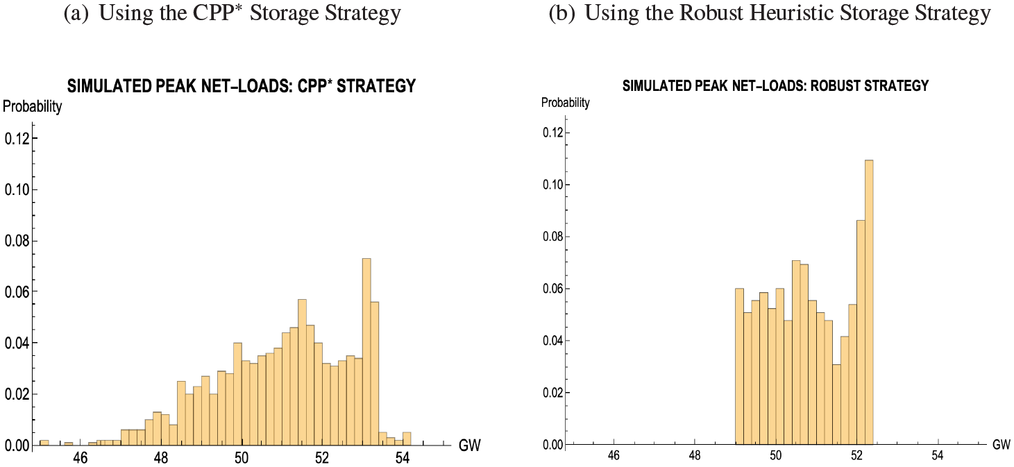
The Simulated Daily Peak Net-Loads

Table 3:

Realized Cost of Energy Savings and the Peak Net-Loads

Storage Strategy	Mean	St. Dev.	Minimum	Maximum	Range
Savings in Energy Costs	million$/day
CPP* Strategy	4.34	0.10	4.00	4.73	0.73
Robust Strategy	1.34	2.28	-3.33	6.03	9.36
Peak Net-Load	GW
CPP* Strategy	50.99	1.67	45.07	54.02	8.96
Robust Strategy	50.16	1.19	49.00	52.40	3.40

Using the CPP* strategy in Figure 12(a), the realized savings vary little around a mean of $4.3 millionIday, with a range of only $0.73 millionIday. In contrast, the variability of the savings using the Robust strategy in Figure 12(b) is much larger with a range of $9.36 millionIday, and the mean savings is only $1.34 millionIday. From the perspective of the owners of distributed storage, it is clear that the distribution of savings using the CPP* strategy would be preferred.

The results for the two storage strategies are completely different for the peak net-load. The maximum peak net-load is lower and the distribution of peak net-loads is more compact using the Robust strategy. The lower maximum peak (50.42 GW versus 52.40 GW) implies that less conventional generating capacity is needed to maintain adequacy. The smaller range of the peak using the Robust strategy (3.40 GW versus 8.96 GW) implies that less reserve capacity for ramping is needed to maintain operating reliability. From the perspective of a system operator, the Robust strategy would be preferred.

These results demonstrate the basic economic trade-off between the two storage strategies. Relying entirely on the price signals from CPP using the CPP* strategy increases and stabilizes the daily savings from purchases of energy in the wholesale market, but it does not mitigate the uncertainty of wind generation. Using the Robust strategy, savings in the wholesale market are sacrificed in order to provide ramping to mitigate the uncertainty of wind generation, and more importantly, to get the maximum attainable reduction of the peak net-load. From a regulatory perspective, the Robust strategy fulfills the initial objective of using distributed storage more effectively to reduce the attainable peak net-load and save capital costs. It seems unlikely, however, that the owners of storage would be willing to accept a higher average cost of energy purchases and more risk in this daily cost without receiving substantial compensation for their contribution to reducing long-run and short-run system costs.

The next section presents the summary and conclusions of the paper, and it raises an important question for future research, namely, who does and who should bear the cost of maintaining the reliability of the grid?

5. Summary and Conclusions

The traditional principle for managing an electric grid was to treat load as an exogenous input and ensure that there was always sufficient supply capacity to meet this load. Consequently, planning decisions were based on forecasts of the annual peak load a few years ahead. Inevitably, this led to the current situation with many installed generating units having low annual capacity factors. In our application to the New York and New England systems, generation from units that are dispatched for less than 100 hours annually represent over 10 percent of the peak load. The economic inefficiency of this type of situation from a long-run perspective has been recognized in the literature for well over fifty years (see Section 2). The typical recommendation for regulators is that customers should pay higher prices for energy purchases during peak load periods. The rationale is based on standard demand response, implying that customers will purchase less and lower the peak when the price is higher. Although this argument is well-established, the implementation of effective rate structures to reduce the peak has only had modest success. Nevertheless, the increasing availability of distributed storage capacity has made it feasible to do a much better job at reducing the peak net-load, and the large savings in capital costs from doing this is the primary motivation for this paper.

In the analysis of a deterministic case in Section 3, a forecast of wind generation is used to determine the daily net-load profile for the peak-load day, and the supply curve is specified to be a linear function of the net-load. The optimal use of storage flattens the daily profile of net-load, shifting load from the peak period in the afternoon to the off-peak period at night. In our example, the storage is represented by deferrable demand, and specifically, by using thermal storage to replace air conditioners for space cooling. This is a relatively inexpensive form of storage compared to batteries. It is important to make a clear distinction between demand response and deferrable demand. With demand response, customers purchase less energy when the peak prices are increased by, for example, setting thermostats higher on hot days. In contrast, with thermal storage the total energy used by customers for cooling remains the same, but the amount of energy purchased increases. ²⁸ Buildings are cooled just as effectively during the day, and in this respect, deferrable demand is non-invasive and does not require customers to accept higher interior temperatures to reduce the peak net-load. ²⁹

The results for the deterministic case derive the optimum short-run condition for using storage to minimize the total daily cost of energy purchases. It implies that the energy price for discharging compared to the price for charging must be high enough to cover the round-trip inefficiency of storage. However, adding capital costs to derive the long-run optimum leads to corner solutions. If just the capital cost of storage is included, it is not economic to install any storage capacity, but if the savings in the capital cost of generating capacity is included as well, it is profitable to use as much deferrable demand as possible to flatten the daily profile of net-load.

The analysis for the stochastic case in Section 4 shows how distributed storage can provide ramping services to mitigate the variability of wind generation as well as shift the net-load to reduce the peak. These two uses compete with each other. We assume that the storage is managed by aggregators who submit bids into the wholesale market, and their objective is to minimize the expected daily cost of the energy purchased from the grid, subject to meeting their customers' demand for energy services. Given the stochastic characteristics of the forecasted price, the optimum bids for storage have a simple structure. If the price is higher than a high threshold, storage is discharged, and if the price is lower than a low threshold, storage is charged. When the price is in between these two thresholds, all customers' energy needs are met by purchasing energy directly from the grid. This latter situation indicates that storage is available for ramping.

The results in Section 4.2 show that when supply is inelastic, the hourly probabilities for either charging or discharging are close to one, and most storage capacity is used to shift load. In contrast, when supply is elastic, the ramping probability is large, and consequently, ramping is more important than shifting load, and if supply is elastic on the peak-load days, the storage will be used inefficiently from a long-run perspective. The main objective of Section 4 is to determine how to manage distributed storage to ensure that it is long-run efficient when the supply is elastic. Since the price signals with elastic supply do not fulfill this objective, some form of intervention is required, and the analysis evaluates Critical Peak Pricing (CPP) as one example.

The stochastic characteristics of wind generation are represented by a simple AR[1] model that exhibits a high degree of positive auto-correlation, and this is consistent with the main characteristics found in our econometric analysis of wind speeds for different locations in the Northeastern states. Although the fit is poor (R² = 10%), there is a lot of useful information in the current residual, and the Pseudo R² is 80% for a one-hour ahead forecast. In our specification, the standard deviation of wind generation is relatively small for the one-hour ahead forecast but it is over twice as large for forecasts more than six hours ahead. Since the supply price is a linear function of the realized net-load, it is higherIlower when the wind generation is lowerIhigher than expected. The relative importance of ramping versus shifting load depends on the price difference between the peak and off-peak periods and how responsive the price is to the realized amount of wind generation.

Implementing CPP provides a substantial incentive to shift energy purchases away from the peak period, and using the forecasted peak reduction as the metric, the results in Table 2 confirm the standard conclusion in the literature. Using CPP* ³⁰ with elastic supply performs similarly to the case with inelastic supply and offsets the poor results for the case with elastic supply but no CPP. The main contributions of this paper are (1) to show why the forecasted peak reduction is an unreliable metric for comparing performance, (2) to define a new metric that is reliable, and (3) to demonstrate how storage can be can be managed to maximize the peak reduction using this new metric. The basic premise is that the performance of a storage strategy should consider different realizations of wind generation. A strategy that works well for the forecasted net-load may perform poorly in more extreme situations when wind generation is lower than expected.

The new metric is based on the definition of "generation adequacy" used by the NERC to assess the future reliability of the high-voltage grid, and this concept is discussed in more detail in Section 4.3. The empirical analysis is based on 1000 simulations of the daily realizations of wind generation, and the different storage strategies are evaluated for all of these simulated days. When wind generation is lower than expected, the deviations from the forecasted net-load represent the up-ramping needed to meet the realized net-load. A simple example in Appendix 7 shows that the maximum "attainable" reduction of the expected peak net-load that meets NERC standards for adequacy is:

$$\mathrm{Max}\left[\mathrm{Attainable}\mathrm{Peak}\mathrm{Reduction}\right]=\left(\mathrm{Max}\left[\mathrm{Discharge}\mathrm{Rate}\right]-\mathrm{Up}-\mathrm{Ramping}\mathrm{at}\mathrm{Peak}\right)$$

(25)

Any attempt to reduce the expected peak further is offset by committing more reserve generating capacity for up-ramping, and the total amount of installed generating capacity required for adequacy remains the same. The realized peak reduction using the Robust strategy is:

$$\mathrm{Realized}\mathrm{Reduction}=\mathrm{Max}\left[\mathrm{Min}\right[\left(\mathrm{Realized}\mathrm{Net}-\mathrm{Load}-\mathrm{Target}\mathrm{Net}-\mathrm{Load}\right),\mathrm{Max}\left[\mathrm{Discharge}\right]\left],0\right]$$

(26)

This result is illustrated in Figures 11(a) and 16, and it implies that the minimum simulated peak reduction is a more reliable metric for assessing generation adequacy than the forecasted peak reduction. The simulated minimum reduction is consistent with the NERC standard for adequacy, and it corresponds to the simulated "worst case" with the lowest realized wind generation.

The important conclusion for regulators is that the potentially substantial savings in the capital cost of generating capacity should be measured by the minimum peak reduction, and the forecasted reduction may exaggerate the benefits. This is illustrated in Table 2. The forecasted peak reductions for inelastic and elastic supply are 5.89 GW and 2.64 GW, respectively. The attainable reductions (simulated minimum) are only 1.32 GW for inelastic supply and -3.48GW for elastic supply. These values are much smaller than the forecasted reductions, and the difference between them is much larger, implying that the adverse effects of elastic supply are exacerbated. Even though the attainable reduction for elastic supply with CPP* is positive (0.90GW), it is still disappointingly small.

We propose a "robust heuristic" strategy that only discharges storage to bring the realized net-load down to a target net-load set by regulators (49 GW). Using this strategy, the attainable reduction is 2.52 GW, and we show that this is the maximum attainable reduction. ³¹ The conclusion is that the Robust strategy reduces the net-capital costs substantially more than the CPP* strategy, and is more long-run efficient than the CPP* strategy. There is, however, an opportunity cost for the owners of distributed storage who adopt the Robust strategy. The results in Section 4.6 show that the CPP* strategy provides larger and more stable savings in the cost of energy purchases than the Robust strategy, and consequently, the CPP* strategy is likely to be preferred by owners.

The analysis in Section 4 implicitly assumes that the regulators are facing a planning problem, and a decision is needed about how to deal with the increasing uncertainty of daily operations for a system where the load is growing. In other words, what is the best investment in new equipment to ensure that the system will meet adequacy standards? The standard economic strategy would be to find sources of generation with high operating costs and low capital cost to provide the up-ramping needed for the peak net-load. In other words, storage is not the best economic solution. With increasing generation from renewable sources, the peak net-load may be falling even though the total load is growing. Consequently, there will be installed conventional units that have been displaced by renewable generation but could still provide the up-ramping needed at the peak. These units will have very low capacity factors, but the capital costs have already been sunk. This appears to be the policy that is now emerging in California, and this is probably a less costly strategy than investing in new distributed storage to provide the up-ramping services required on peak days. The installed generating capacity needed for adequacy will be larger than it could be, and it may require some form of capacity payment to ensure that it is available when needed.

If one accepts the argument that it is highly likely that the owners of distributed storage will adopt the CPP* strategy rather than the Robust strategy, an alternative approach to lowering the requirements for adequacy is desirable. The most direct way to accomplish this is to reduce the amount of up-ramping required at the peak by using more accurate forecasts of renewable generation. For example, we have advocated using a receding-horizon optimization to replace a day-ahead commitment. This implies that the optimum dispatch is always based on a one-hour ahead forecast. Since the standard deviation of the one-hour ahead forecast is half the size of the standard deviation for forecasts more than six hours ahead, the amount of generating capacity committed for ramping in our example would also be halved. Furthermore, allowing the managers of distributed storage to update their bids for every time period makes it feasible for them to ensure that the capacity constraints for their storage are never violated.

If the Robust strategy for storage is rejected, the challenge of determining how to allocate the cost of the increased risk of daily operations on the grid remains. Eventually, customers will get the bill for supporting any additional generating capacity that is needed for adequacy. Nevertheless, we believe that the grid of the future will benefit from making load more responsive to the real-time availability of renewable generation. To do this, it will be important to recognize that renewable generation is not perfectly fungible with conventional generation. There will be times when there is surplus renewable generation and the marginal supply cost is zero. Customers with distributed storage should be exposed to these low prices to provide the incentive for them to use their storage efficiently. Finding additional ways to make net-load offset the increased uncertainty caused by higher levels of renewable generation, such as producing "green hydrogen," should be a high priority for future research.