Sage Journals: Discover world-class research

Abstract

In this paper, we consider a simultaneous modeling of good and bad outputs. We use an input distance function (IDF) with endogenous inputs as well as endogenous bad outputs, which is novel in the literature. Moreover, we model input efficiency to depend on the production of bad outputs which allows us to investigate whether emissions of pollutants (bad outputs) are related to technological performance (technical efficiency). We also model production of each bad output with a spatial structure separately, each depending on production of good outputs, inputs and other exogenous variables. These bad output production functions allow us to estimate both direct and indirect effects of good output on the production of bad outputs, which may be of special interest because they show the cost (to the society) in terms of releasing pollutants to the environment in order to increase production of good outputs. We apply the new technique to a data set on U.S. electric utilities with four bad outputs, three inputs and two good outputs. We used a Bayesian technique to estimate the model which is a system consisting of the input distance function, reduced form equations for each input, dynamics of inefficiency and bad output production technology—separately for each. Empirically, bad outputs are found to affect inefficiency positively. Percentage increases in inefficiency due to a percentage increase in each bad output are found to vary from 0.225% to 0.42%. Energy prices are found to be positively related to inefficiency. From the spatial specifications of bad outputs, we find that the spillover effects of increasing production of good outputs account for the majority of the total effect, indicating that neighborhood effects are more important than own effects. This means, the neighboring utilities played a crucial role indicating “contagion” of practices.

Keywords

Environmental pollution Bad outputs Input distance functions Monte Carlo methods

1. Introduction

In many production processes production of desirable (good) outputs also produce some unintentional (undesirable or bad) outputs. Electric power generation is one such example. This unintentional but inevitable outcome is labeled as “bi-production” (BP). The modeling of production technology that use undesirable outputs follows two distinct strands. In the directional distance function and transformation function approaches (see Färe et al. (2005), Atkinson and Dorfman (2005), Fernández et al. (2005), Agee et al. (2014), among others), the technology is specified by a single equation in which good and bad outputs as well as inputs enter as arguments. On the contrary, the BP approach consists of separate production technologies for good and bad outputs.

In this paper we use a modeling approach that relies on the BP concept introduced in Murty et al. (2012), Førsund (2009) and Fernández et al. (2002), Kumbhakar and Tsionas (2016). The technology for the production of good outputs is specified in terms of a standard translog input distance function (IDF) with input-oriented technical inefficiency. We depart from the Kumbhakar and Tsionas (2016) model by including bad outputs in the IDF. Our by-production technologies depend on good outputs. Thus we consider simultaneity between good and bad outputs. That is, similar to a single equation representation of the technology our IDF depends on bad outputs also. Other distinguishing features of our models are as follows. (i) We use a very flexible and dynamic inefficiency model. Inefficiency is allowed to depend on the current and past inefficiency of nearby electric plants via a spatial structure. It also depends on some exogenous variables and more importantly on bad outputs. (ii) Production of bad output technologies are specified as SAR models, each bad output with its own spatial autoregressive (SAR) parameters. The exogenous variables in these functions are good outputs and some other environmental variables (which are ideally inputs used to mitigate production of bad outputs).

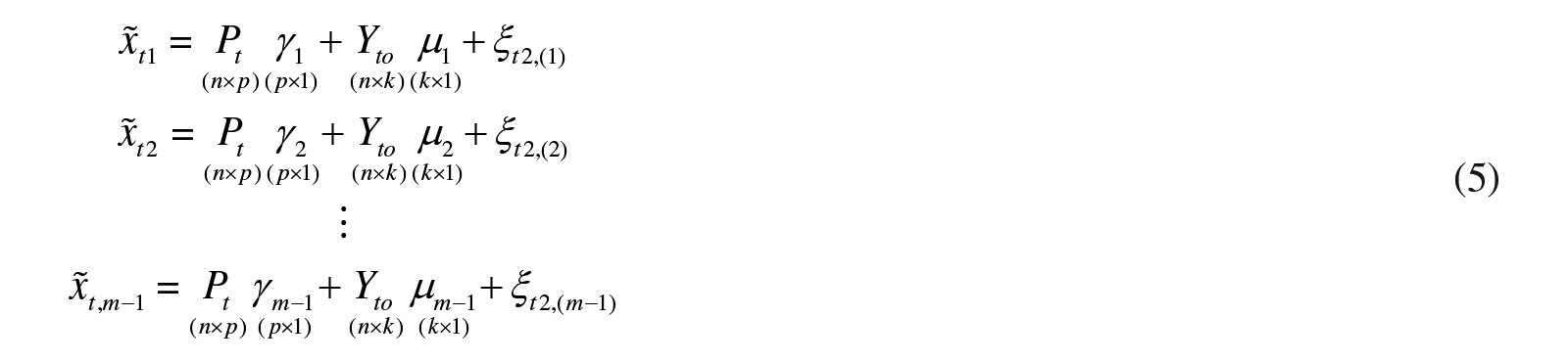
Since we allow simultaneity between good and bad outputs in the IDF, it cannot be estimated directly because of endogeneity of bad outputs and possible endogeneity of input ratios (that appear in the IDF because it is homogeneous of degree 1 in inputs). To control for these endogeneity, following the BP approach, we add separate technologies for the production of each bad output which also depends on quantity of good outputs produced. Thus, the simultaneity between good and bad outputs are addressed by using a system approach, in contrast to the single equation approach in Färe et al. (2005), Atkinson and Dorfman (2005) in which endogeneity is not corrected. The main advantages of doing this are as follows. (i) We can compute the shadow price of each bad outputs from $\partial Y_{g} / \partial B_{m}$ where $Y_{g}, g = 1, \dots, G$ are G good outputs and $B_{m}, m = 1, \dots, M$ are M bad outputs. These shadow prices indicate sacrifice of good outputs for an increase in production of each bad output.¹ Unlike electricity, emissions without regulations are non-marketable goods in the sense no producer/consumer will be interested in buying them. This does not mean they are free at least from the societal point of view. So unobserved prices are often predicted/estimated from shadow prices, which from a production function perspective is defined as the reduction of good output(s) for an increase in bad output(s). Since good outputs have market prices, one can evaluate the monetary cost of an increase in bad output(s) multiplying $\partial Y_{g} / \partial B_{m}$ by the price of Y_g. These shadow prices can be useful to the regulators because they can impose a tax on emissions based on these shadow prices. (ii) From the bad output technologies, we can compute $\partial B_{m} / \partial Y_{g}$ (which can be decomposed into a direct and indirect effect because of the spatial structure on each). The partials for each m and g show the societal cost (in terms of releasing pollutants which are the bad outputs) in producing more good outputs. These can also viewed as negative externality of producing good outputs. Since our models have a spatial structure, these shadow prices have a direct and indirect effect.

Note that here we are using an IDF from which we can compute the marginal effects each bad output on cost represented by the IDF ( $\partial X_{1} / \partial B_{m}$ or its elasticity $\partial 1 n X_{1} / \partial 1 n B_{m}$ ). Since the IDF is homogeneous of degree 1 in inputs, if $\partial 1 n X_{1} / \partial 1 n B_{m} = a$ the cost will decrease by $a %$ for a decrease in B_m by $a %$ . Thus, we can give a cost interpretation of these derivatives. That is, the shadow prices are translated to cost in an IDF. In other words, these derivatives show by how much cost can be reduced by reducing each types of emission. One can also write $\partial 1 n X_{1} / \partial 1 n B_{m}$ as the product of $\partial 1 n X_{1} / \partial 1 n Y_{g}$ and $\partial 1 n Y_{g} / \partial B_{m}$ , where the first term can be viewed as cost elasticity of good output (because of the duality between the IDF and cost function) and the second term is related to the the shadow price of B_m.

There are several papers that deal with the issue in general terms in a stochastic frontier (SF) framework. For example, Atkinson, Primont and Tsionas (2018) compute optimal directions subject to profit maximization and cost minimization, correct for the potential endogeneity of inputs and outputs, estimate latent prices for bad outputs, measure firms’ responses to shadow prices rather than actual prices, and introduce an unobserved productivity term. They also apply their techniques to U.S. electric utilities. Atkinson and Tsionas (2018) include parameters to estimate optimal directions which correspond to the firm’s profit-maximizing (PM) position and generalize the directional distance function (DDF) to a shadow-quantity DDF. To estimate the shadow quantities and the structural parameters, they form the shadow DDF system, which includes the shadow DDF and all the first-order price equations from the shadow-PM problem. Note that these papers are not directly related to what we do here. Because none of them deal with spatial models with dynamics, and endogeneity of both good and bad outputs as well as inputs. Our model is quite flexible and technically sophisticated. Kumbhakar and Tsionas (2016, hereafter KT) is the first paper that use IDF and address endogeneity of inputs in a bi-production model. However, although they use panel data in their application, their models did not use any panel features and there was no dynamics.²

There are other papers in the literature that use the non parametric DEA approach, such as Bigerna et al. (2020) that accounts for Greenhouse gas emissions as bad output and Bigerna et al. (2019) which estimates the spatial effects on efficiency. Unfortunately our literature survey is not exhaustive primarily because we focus on bi-production spatial econometric models with good and bad outputs first, and then endogeneity of inputs and outputs (both bad and good) with dyanmic inefficiency. Although there are some papers in the first category which we cited above, there are no papers that deal with both. And that is where our contribution is in this paper. Our main contributions are as follows. First, we consider a true simultaneous model (not a triangular one as in KT) in which production of good output depends on the bad outputs and vice-versa. We introduce separate equations to represent the technology of the good output production (in terms an IDF), and separate technologies for the production of each bad outputs. Input oriented technical inefficiency is made dynamic by not only allowing inefficiency to depend on its past values but also on some exogenous variables and production of bad outputs. We assume that the input ratios in the IDF are endogeous and introduce a system of equations with exogenous instruments. Finally, we use a Bayesian method to estimate the system.

2. Model

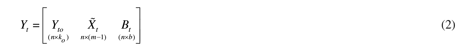
We specify the production technology in terms of a transformation function $F (Y_{t}, X_{t}) = A_{t}$ (Kumbhakar (2013)), an input distance function (IDF) representation of which after using the homogeneity of degree one condition (in inputs) is³

x_{t 1} = Y_{t} β + v_{t} + e^{s_{t}},

(1)

where $x_{t 1}$ is $n \times 1$ is the normalizing input (e.g., labor), $Y_{t}$ is an $n \times k$ matrix defined below, $β$ is a $d_{β} \times 1$ vector of parameters, $v_{t}$ is an $n \times 1$ error term, and $s_{t}$ is an $n \times 1$ stochastic component that is related to input oriented inefficiency $u_{t}$ , defined as $u_{t} = \exp (s_{t})$ or $s_{t} = \log u_{t}$ as in Tsionas (2006). The $Y_{t} β$ is is the deterministic frontier (IDF) which is represented by either by a Cobb-Douglas or a translog function. The $Y_{t}$ matrix includes

Y_{t} = [\begin{matrix} \underset{(n \times k_{0})}{Y_{t 0}} \underset{n \times (m - 1)}{{\tilde{X}}_{t}} \underset{(n \times b)}{B_{t}} \end{matrix}]

(2)

where $Y_{0}$ contains good outputs. In the case of $m$ inputs

{\tilde{X}}_{t} = [x_{t 2} - x_{t 1}, \dots, x_{tm} - x_{t 1}] = [{\tilde{x}}_{t 1}, \dots, {\tilde{x}}_{t, m - 1}],

(3)

where the lowercase letters are logarithms of uppercase letters, and $B_{t}$ is a matrix of observations on bad outputs. For technical inefficiency we assume

s_{t} = ρ_{1} W s_{t} + ρ_{2} W s_{t - 1} + \underset{(n \times d_{z})}{Z_{t}} γ_{(d_{z} \times 1)} + \underset{(n \times b)}{B_{t}} ω_{(b \times 1)} + ξ_{t 1}

(4)

where $W$ is the $n \times n$ proximity matrix, $Z_{t}$ is an $n \times d_{z}$ matrix of observations on exogenous variables and associated parameters $γ$ , $ρ_{1}$ and $ρ_{2}$ are SAR parameters, $ω$ is a $b \times 1$ vector of parameters associated with $B_{t}$ , and $ξ_{t}$ is an $n \times 1$ error term. Our modeling on inefficiency in (4) is quite general. First, it is dynamic and includes inefficiency of current as well as past inefficiencies. Second, it depends on other exogenous variables $Z_{t}$ . Third, it depends on the amount of bad outputs produced. Finally, there is the unexplained part, $ξ_{t 1}$ . We allow the input ratios (in log) to be endogenous and specify them as functions of variables that are exogenous (instruments), viz.,

\begin{matrix} {\tilde{x}}_{t 1} = \underset{(n \times p)}{P_{t}} \underset{(p \times 1)}{γ_{1}} + \underset{(n \times k)}{Y_{t 0}} \underset{(k \times 1)}{μ_{1}} + ξ_{t 2, (1)} \\ {\tilde{x}}_{t 2} = \underset{(n \times p)}{P_{t}} \underset{(p \times 1)}{γ_{2}} + \underset{(n \times k)}{Y_{t 0}} \underset{(k \times 1)}{μ_{2}} + ξ_{t 2, (2)} \\ ⋮ \\ {\tilde{x}}_{t, m - 1} = \underset{(n \times p)}{P_{t}} \underset{(p \times 1)}{γ_{m - 1}} + \underset{(n \times k)}{Y_{t 0}} \underset{(k \times 1)}{μ_{m - 1}} + ξ_{t 2, (m - 1)} \end{matrix}

(5)

where $P_{t}$ contains data on exogenous variables and $γ_{j}$ are $p \times 1$ parameters $(j = 1, \dots, m - 1)$ . The $ξ_{t 2, (1)}, \dots, ξ_{t 2, (m - 1)}$ are random terms. The above equations can also be viewed as reduced form expressions without specifying the structural model and/or behavioral assumptions such as profit maximization or cost minimization. We write these equations compactly as

\underset{n (m - 1) \times 1}{{\tilde{X}}_{t}} = (I_{m - 1} \otimes P_{t}) γ_{p (m - 1) \times 1} + (I_{k} \otimes Y_{t 0}) μ_{((m - 1) k \times 1)} + ξ_{t 2},

(6)

where $γ = [{γ'}_{1}, \dots, {γ'}_{m - 1}], μ$ is the vector of coefficients corresponding to $(I_{k} \otimes Y_{t 0})$ . Its elements are denoted by $μ = [μ_{j}]$ . For the bad outputs we assume:

\begin{matrix} \underset{(n \times 1)}{B_{t 1}} = λ_{1} W B_{t 1} + \underset{(n \times q)}{Q_{t}} \underset{(q \times 1)}{δ_{1}} + \underset{(n \times m)}{X_{t}} \underset{(m \times 1)}{ϕ_{1}} + \underset{(n \times k)}{Y_{t}} \underset{(k \times 1)}{ψ_{1}} + ξ_{t 3, (1)}, \\ \underset{(n \times 1)}{B_{t 2}} = λ_{2} W B_{t 2} + \underset{(n \times q)}{Q_{t}} \underset{(q \times 1)}{δ_{2}} + \underset{(n \times m)}{X_{t}} \underset{(m \times 1)}{ϕ_{2}} + \underset{(n \times k)}{Y_{t}} \underset{(k \times 1)}{ψ_{2}} + ξ_{t 3, (2)}, \\ ⋮ \\ \underset{(n \times 1)}{B_{tb}} = λ_{b} W B_{tb} + \underset{(n \times q)}{Q_{t}} \underset{(q \times 1)}{δ_{b}} + \underset{(n \times m)}{X_{t}} \underset{(m \times 1)}{ϕ_{b}} + \underset{(n \times k)}{Y_{t}} \underset{(k \times 1)}{ψ_{b}} + ξ_{t 3, (b)}, \end{matrix}

(7)

where $Q_{t}$ contains exogenous variables, $λ_{j}$ are spatial dependence parameters, and

X_{t} = [x_{t 1}, {\tilde{x}}_{t 1}, \dots, {\tilde{x}}_{t, m - 1}] .

(8)

These equations can be written in the form

\begin{matrix} (I_{n} - λ_{1} W) \underset{(n \times 1)}{B_{t 1}} = \underset{(n \times q)}{Q_{t}} \underset{(q \times 1)}{δ_{1}} + \underset{(n \times m)}{X_{t}} \underset{(m \times 1)}{ϕ_{1}} + \underset{(n \times k)}{Y_{t}} \underset{(k \times 1)}{ψ_{1}} + ξ_{t 3, (1)}, \\ (I_{n} - λ_{2} W) \underset{(n \times 1)}{B_{tb}} = \underset{(n \times q)}{Q_{t}} \underset{(q \times 1)}{δ_{b}} + \underset{(n \times m)}{X_{t}} \underset{(m \times 1)}{ϕ_{b}} + \underset{(n \times k)}{Y_{t}} \underset{(k \times 1)}{ψ_{2}} + ξ_{t 3, (b)}, \\ ⋮ \end{matrix}

(9)

These are compactly written as

(I_{n} - λ_{b} W) \underset{(n \times b)}{B_{t}} = (I_{b} \otimes Q_{t}) δ + (I_{b} \otimes X_{t}) ϕ + (I_{b} \otimes Y_{t}) ψ_{(bk \times 1)} + \underset{(nb \times 1)}{ξ_{t 3, (b)}},

(10)

where $δ_{(qb \times 1)} = [{δ'}_{1}, \dots, {δ'}_{n}]$ , $ξ_{t 3} = [{ξ'}_{t 3, (1)}, \dots, {ξ'}_{t 3, (b)}]$ . Define

A_{(n^{2} \times n)} = [\begin{matrix} I_{n} - λ_{1} W \\ I_{n} - λ_{1} W \\ \begin{matrix} ⋮ \\ I_{n} - λ_{b} W \end{matrix} \end{matrix}]

(11)

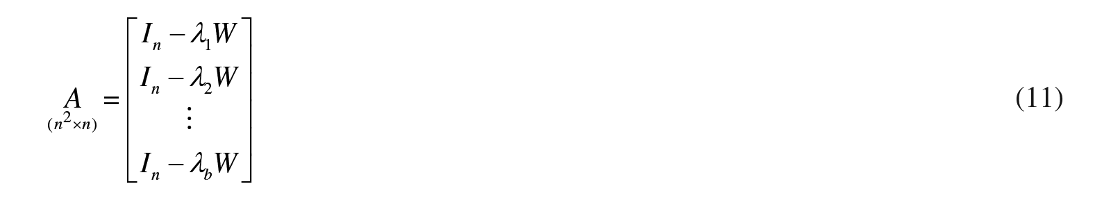
and write (10) as

A_{(nb \times nb)} \underset{(nb \times 1)}{B_{t}} = (I_{b} \otimes Q_{t}) δ + (I_{b} \otimes X_{t}) ϕ + (I_{b} \otimes Y_{t}) ψ + \underset{(nb \times 1)}{ξ_{t 3}} .

(12)

Denote by $ϕ_{Y 1} = [ϕ_{1, (1)}, ϕ_{2, (1)}, \dots, ϕ_{b, (1)}]$ , i.e., the coefficients of (7) corresponding to $x_{t 1}$ . Given that $W$ is normalized, we need the following regularity condition on $ρ$ ( $ρ_{1} = ρ$ and $ρ_{2} = 0$ in the simple case without lag $W$ ), i.e., $1 / λ_{\max} < ρ < 1 / λ_{\min}$ where $λ_{\max}$ and $λ_{\min}$ are the largest and smallest eigen values of $W$ . For the general case, $1 / λ_{\max} < ρ_{1} < 1 / λ_{\min}$ , and $ρ_{2}$ is between (0,1).⁴

Marginal effects of inefficiency can be derived as follows. Since we specified inefficiency as a dynamic process, it should have a steady-state value that is finite. If we denote the steady-state values of $s_{t}$ and $Z_{t}$ by $s_{*}$ , $Z_{*}$ , then the marginal effects in the long-run or steady state are

\frac{\partial s_{*}}{\partial {Z'}_{*}} = {(I - (ρ_{1} + ρ_{2}) W)}^{- 1} γ .

(13)

In the short-term we have

\frac{\partial s_{t}}{\partial {Z'}_{t}} = {(I - ρ_{1} W)}^{- 1} γ .

(14)

The marginal effects of variables in $Q_{t}$ on bad output $B_{tj}$ are

\frac{\partial B_{tj}}{\partial {Q'}_{t}} = {(I_{n} - λ_{j} W)}^{- 1} δ_{j}, j = 1, \dots, m .

(15)

The marginal effects of variables in $X_{t}$ (see (8) on bad output $B_{tj}$ are computed as follows. First, a change in $ξ_{t 2, j}$ affects ${\tilde{x}}_{j}$ through (5), which in turn affects $B_{tt}$ through (7), and finally, $x_{t 1}$ in (1). So, we have two effects, one from (7) and one from (1). Second, a change in $ξ_{t 3, j}$ affects bad output $B_{th}$ through (7), and $x_{t 1}$ through (1). So, there are different effects on $x_{t 1}$ and ${\tilde{x}}_{tj} . s (j = 1, \dots, m - 1)$ . As the error terms are correlated as in (16), these effects can be computed numerically using the Generalized Impulse Response Function (GIRF) (see Koop et al. (1996) and Pesaran and Shin (1998)). Our stochastic assumptions are as follows:

V_{t} = (v_{t}, {ξ'}_{t 1}, {ξ'}_{t 2}, {ξ'}_{t 3}) ~ N_{d} (0, \sum),

(16)

where the dimensionality $d = n (1 + 1 + m - 1 + b) = n (m + b + 1)$ We denote the parameter vector by

θ = (β', γ', δ', ϕ', μ', ψ'),

(17)

whose dimensionality is $d_{θ} = d_{β} + m (p + b) + bq + k (b + p)$ . Our prior on $θ$ is proper but diffuse, i.e., $θ ~ N_{d_{θ}} (0, h^{2} I_{d_{θ}})$ , where we set $h = 10$ . For ∑ we assume an inverted Wishart prior (Zellner, 1971, p. 395):

p (\sum | θ) \propto | \sum |^{- (d_{\sum} + \bar{N} + 1) / 2} \exp {- \frac{1}{2} tr \bar{A} \sum^{- 1})},

(18)

where $d_{\sum} = m + b + 1$ , $\bar{A} = \bar{a} I_{d_{\sum}} (\bar{a} = 0.01)$ and $\bar{N} = 1$ . This is, again, a proper but quite diffuse prior.

The system of equations used for estimation are (1), (4), (5), and (12). Estimation details are reported in the Appendix A. Finally, the decomposition into direct and indirect (spillover) effects is performed as follows. In log form, most marginal effects can be expressed in the generic form as

V = {(I - λ W)}^{- 1} b \equiv Ab,

(19)

where b represents any parameter in the right-hand side of (7) for example. The first row of A, for example, is $A = [a_{11}, a_{12}, \dots, a_{1 n}]$ so $V_{1} = \sum_{j = 1}^{n} a_{1 j} b_{j}$ . We know that all elements of A have to be positive (Kutlu, 2018). Therefore, the own effect is $a_{11} b_{1}$ and the spillover effects (as a percentage) are

v_{i} = \frac{\sum_{j \neq 1}^{n} a_{ij} b_{j}}{\sum_{j = 1}^{n} a_{ij} b_{j}}, j = 1, \dots, n, \dots i = 1, \dots, n, .

(20)

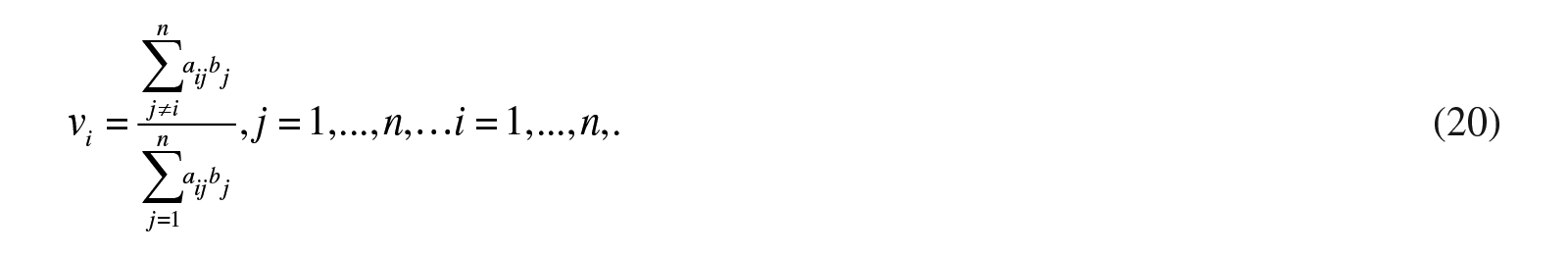
This procedure is repeated to compute marginal effects of all the variables of interest.

3. Data

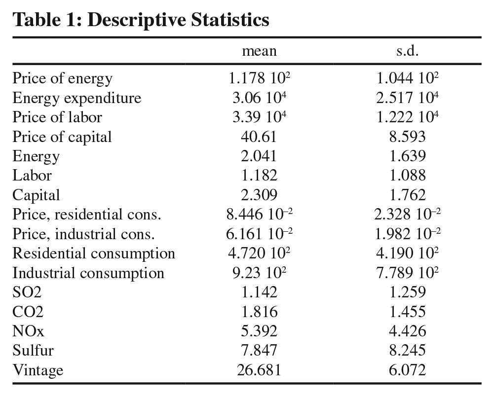
Our data is sourced from Atkinson, Primont, and Tsionas (2018). It contains information on 77 U.S. electric utilities observed during the period 1995–2005. It is an unbalanced panel and contains 1201 plant-year observations. We use three inputs (energy, labor, and capital), two good outputs (residential and industrial/commercial delivery of electricity) and four bad outputs, SO2, CO2, N0x, and sulfur (S). The quantity of energy is measured in total Btu of fuel consumed and the quantity of labor is the number of full-time plus 50% of the part time employees. Capital is measured as the expenses on interest plus depreciation. We also have prices for the inputs and good outputs. In the IDF, labor appears on the left-hand side, and we also include a dummy for privatized utilities and vintage of equipment for each plant. The W matrix was constructed using GIS information. We use the inverse distance weighting formulation

w_{ij} = {\begin{matrix} 1 / d_{ij}^{\propto}, if i \neq j, \\ 0, if i = j, \end{matrix}

with $α = 1$ . The instruments consist of prices, lagged values of inputs and output, including privatization, vintage, and time dummies; the instruments in (7) are the same but include lagged bad outputs as well, and the functional form in (1) is translog including vintage, a restructuring dummy and trend dummies to measure technical change. Here, $x_{t 1}$ is labor, ${\tilde{X}}_{t}$ denote capital and coal, $y_{t 0}$ denotes the two good outputs, while the bad outputs, $B_{t}$ , are SO2, CO2, NOx and S.

Summary statistics of the variables used are given in Table 1.

Table 1

Descriptive Statistics

	mean	s.d.
Price of energy	1.178 10²	1.044 10²
Energy expenditure	3.06 10⁴	2.517 10⁴
Price of labor	3.39 10⁴	1.222 10⁴
Price of capital	40.61	8.593
Energy	2.041	1.639
Labor	1.182	1.088
Capital	2.309	1.762
Price, residential cons.	8.446 10^–2	2.328 10^–2
Price, industrial cons.	6.161 10^–2	1.982 10^–2
Residential consumption	4.720 10²	4.190 10²
Industrial consumption	9.23 10²	7.789 10²
SO2	1.142	1.259
CO2	1.816	1.455
NOx	5.392	4.426
Sulfur	7.847	8.245
Vintage	26.681	6.072

4. Results

4.1 Estimation and results

We use 150,000 Markov Chain Monte Carlo (MCMC; Tierney, 1994) iterations the first 50,000 of which are discarded to mitigate possible start up effects. Moreover, we use 1,000 particles per MCMC iteration. Our details on MCMC are reported in Appendix A. MCMC performance and prior sensitivity are taken up in Appendix B.

4.2 Parameter estimates

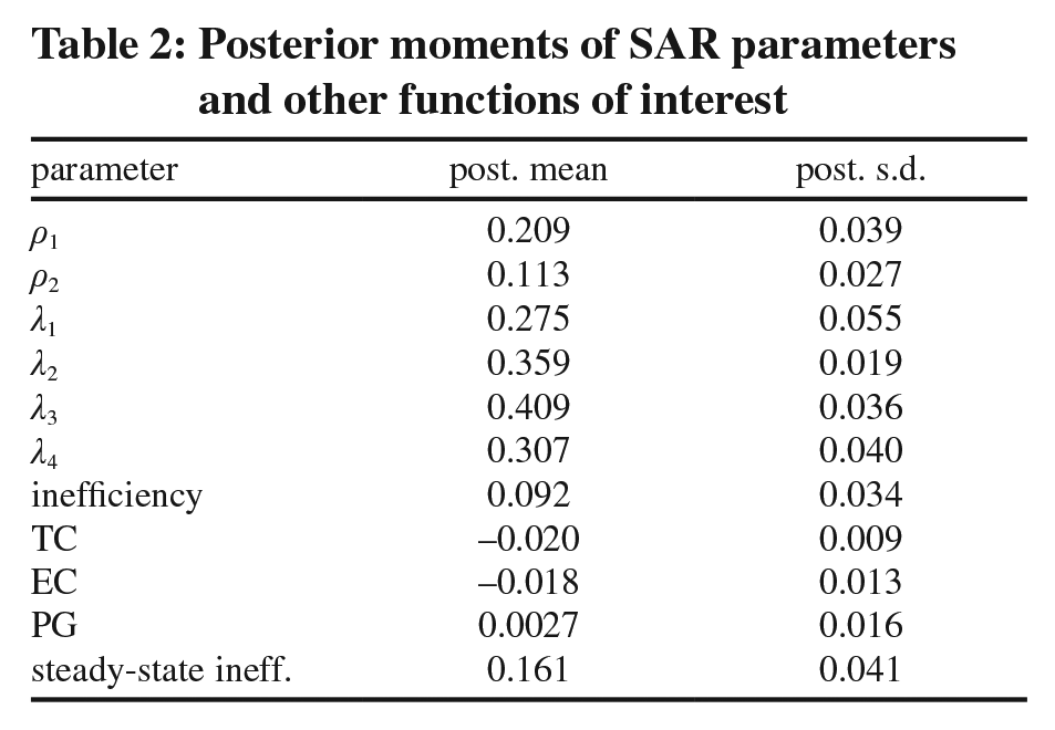
Of special interest are parameters $ρ_{1}$ , $ρ_{2}$ , $λ_{1}$ , $λ_{2}$ , $λ_{3}$ and $λ_{4}$ corresponding respectively, to SO2, CO2, NOx and S.Their posterior moments and densities are presented, respectively, in Table 2 and Figures 1 and 2. These parameters are all statistically significant, thereby justifying that (i) there are spillover effects of present and past inefficiencies, and (ii) there are also spillover effects in the production of each of the bad outputs. The posterior densities of $ρ_{1}$ , $ρ_{2}$ , $λ_{1}$ , $λ_{2}$ , $λ_{3}$ and $λ_{4}$ are reported in Figure 1. It can be seen that some of these parameters have high variances.

Table 2

Posterior moments of SAR parameters and other functions of interest

parameter	post. mean	post. s.d.
$ρ_{1}$	0.209	0.039
$ρ_{2}$	0.113	0.027
$λ_{1}$	0.275	0.055
$λ_{2}$	0.359	0.019
$λ_{3}$	0.409	0.036
$λ_{4}$	0.307	0.040
inefficiency	0.092	0.034
TC	–0.020	0.009
EC	–0.018	0.013
PG	0.0027	0.016
steady-state ineff.	0.161	0.041

Figure 1

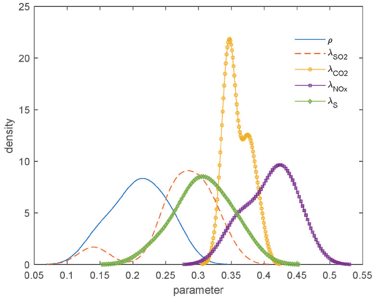
Marginal posterior densities of SAR parameters

Figure 2

Sampling distributions of posterior mean estimates of functions of interest

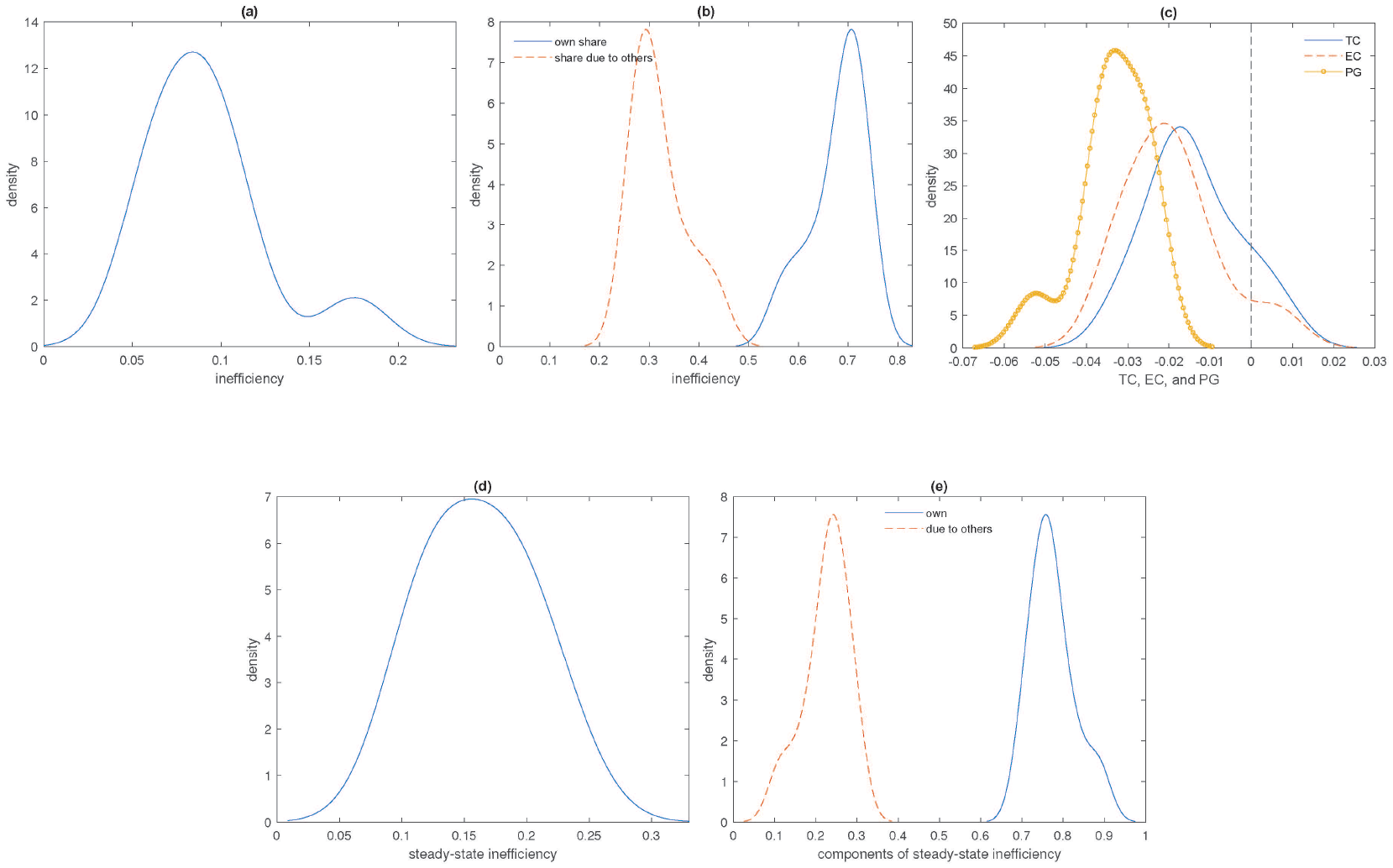
The IDF in (1) includes time dummies. We estimate Technical Change (TC) using the coefficients of time dummies in (1), i.e., $β_{t} - β_{t -}$ where $β_{t}$ is the coefficient of time dummy $D T_{t}$ . Since the IDF is dual to a cost function, a negative (positive) TC will mean technical progress (regress) which is cost diminution (increase), ceteris paribus.

4.3 Efficiency change decomposition

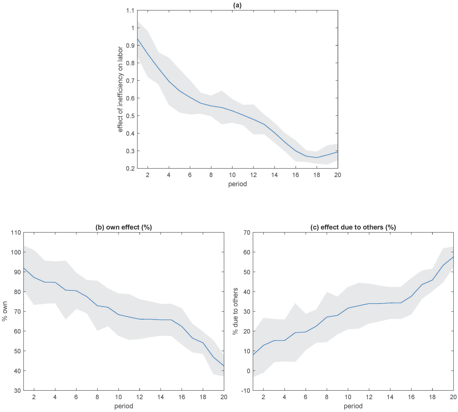
Given efficiency estimates, ${\hat{u}}_{it}$ , Efficiency Change (EC) is computed as $E C_{it} = \exp (- u_{it}) - \exp (- u_{i, t - 1})$ . Note that $u_{it} = \exp (s_{it})$ . The distribution of $u_{it}$ is shown in Figure 2 panel (a). It can be seen that the distribution is bi-modal with mean close to 0.11. Barring some extreme values, inefficiencies are not too high. Given the specification of $s_{t} = ρ_{1} W s_{t} + ρ_{2} W s_{t - 1} + Z_{t} γ + B_{t} ω + ξ_{t 1}$ in (4) inefficiency will have a direct and indirect effect. The direct effect is a firms own inefficiency and the indirect effect comes from neighbors’ inefficiency. In panel (b) we report both the direct and indirect effects. It can be seen from the figures that the average direct effect is about double of the indirect effect. Finally, in panel (c) we report distribution of TC, EC and PG, where PG is productivity growth which is decomposed as $PG = TC + EC$ . Note that negative TC means cost diminution (technical progress). It can be seen from the figure that most of the firms had technical progress. On the other hand, EC is negative for most of the firms thereby meaning that efficiency deteriorated over time. Since negative TC is technical progress, we have $PG = - TC + EC$ .

In part (b) of Figure 2 we report own effects and effects due to others of technical inefficiency for the current period $(t)$ and the previous period $(t - 1)$ . Results are averaged across $t$ and $t - 1$ respectively. In panels (d) and (e) we report the posterior distribution of long-run inefficiency and the contributions of own and neighbor effects in percentage terms. Steady-state inefficiency averages 0.161 (s.d. 0.041), the own effect is 0.774 (s.d. 0.054) while the neighbor effects average 0.226 (s.d. 0.054).

4.4 Marginal effects and shadow prices

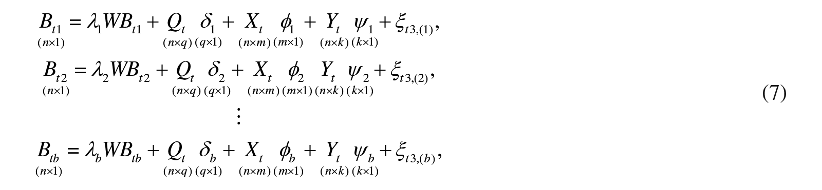
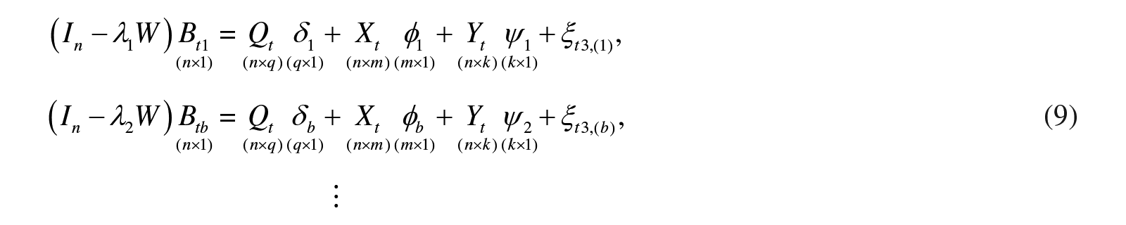
Technologies of the production of bad outputs are specified in (7) (rewritten in (9)). We use (9) to examine the marginal effects of good outputs (residential and commercial use of electricity) on the four bad outputs obtained from these formulas. From (9)

\frac{\partial B_{tj}}{\partial Y_{t}} = {(I - λ_{j} W)}^{- 1} ψ_{j}, j = 1, \dots, b .

(21)

Since $B_{tj}$ and $Y_{t}$ are in logs, these partial effects are in fact elasticities. That is, these marginal effects are shadow prices elasticities. As mentioned in the introduction, the shadow prices indicate the indirect cost of the the bad outputs because these elasticities show by what percent each good output has to be sacrificed for a one percentage increase each bad output. However, the derivatives above are the reciprocal of the shadow prices. We assume monotonocity to take the inverse of the derivatives for shadow prices. The results are presented in Figure 3. Given the spatial nature of the technologies, we separate the own (direct) effects from the indirect effects coming from the neighboring plants. The direct marginal effect of residential electricity demand on SO2 is the highest among the four bad outputs. It varies from from 0.3 to 0.67, i.e., for an increase in residential electricity output by 1%, SO2 increases by 0.3% to 0.67%. The indirect effect is much smaller varying from about 0.1% to 0.17%. For sulfur the direct effects at the lower end are similar to the indirect effects. However, the maximum of the direct effect (0.35%) is bigger than that of the indirect effect (0.23%). The direct and indirect effects of SO2 are quite similar (ranging from 0.05% to 0.25%). Similar is the case with NOx. Panels (c) and (d) report the direct and indirect effects of commercial electricity delivery on each of the four bad outputs. The direct effects on SO2 and Sulfur are the highest followed by CO2 and NOx. The indirect effects are much spread out. For example, the effect on NOx varies from close to zero to 0.32%. The distributions of S and SO2 are somewhat similar, while CO2 distribution is quite tight ranging from 0.15% to 0.27%.

Figure 3

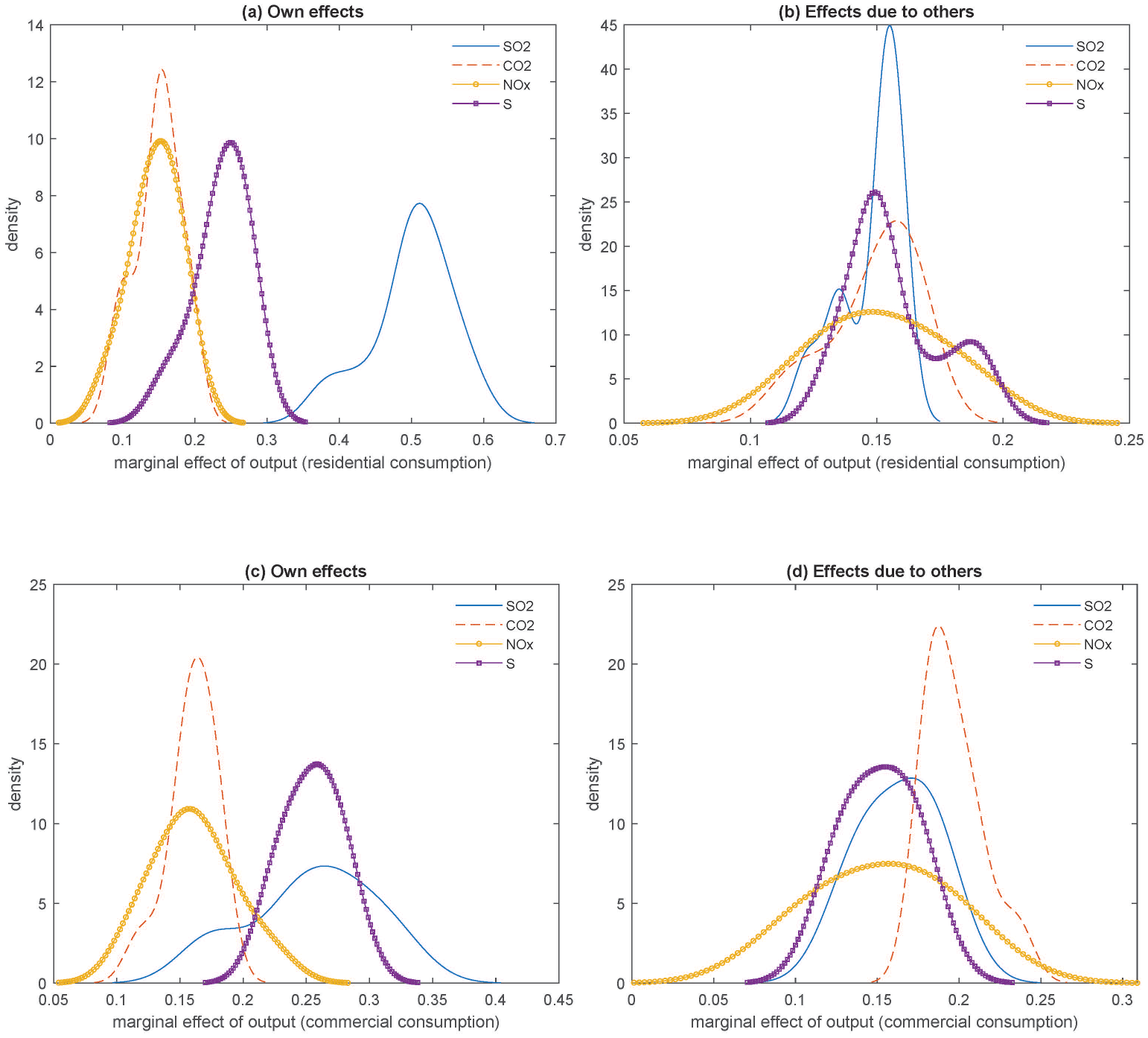
Marginal effects of good output on bad outputs

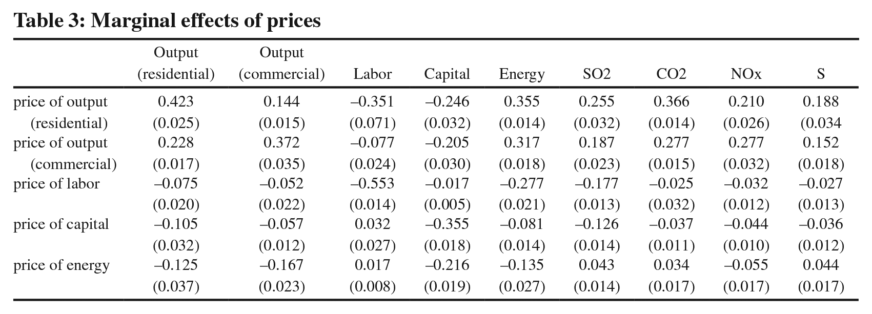
In Table 3, we report marginal effects of prices on labor, good and bad outputs. Note that since the IDF is homogeneous of degree 1 in inputs, the effect on labor is the same as other inputs and therefore on cost. Since prices are used as exogenous variables, it might be of interest to check their marginal effects. So there should be a direct and an indirect effect. The formulas are shown in equations (21) and (22). We report the overall effect (both direct and indirect combined) in Table 2. Marginal effects of output prices on outputs are positive, as expected. Their effect on labor and capital are negative while the effect on energy is positive. The effects on all four bad outputs are positive. An increase in output prices increase supply (production) which in turn increases production of bad outputs. This is expected because it is not possible to reduce bad outputs when the production of good outputs increase. The marginal effects of inputs on outputs are negative because an increase in input prices will reduce their use which will lower production of good and bad outputs.

Table 3

Marginal effects of prices

	Output (residential)	Output (commercial)	Labor	Capital	Energy	SO2	CO2	NOx	S
price of output (residential)	0.423	0.144	–0.351	–0.246	0.355	0.255	0.366	0.210	0.188
	(0.025)	(0.015)	(0.071)	(0.032)	(0.014)	(0.032)	(0.014)	(0.026)	(0.034)
price of output (commercial)	0.228	0.372	–0.077	–0.205	0.317	0.187	0.277	0.277	0.152
	(0.017)	(0.035)	(0.024)	(0.030)	(0.018)	(0.023)	(0.015)	(0.032)	(0.018)
price of labor	–0.075	–0.052	–0.553	–0.017	–0.277	–0.177	–0.025	–0.032	–0.027
	(0.020)	(0.022)	(0.014)	(0.005)	(0.021)	(0.013)	(0.032)	(0.012)	(0.013)
price of capital	–0.105	–0.057	0.032	–0.355	–0.081	–0.126	–0.037	–0.044	–0.036
	(0.032)	(0.012)	(0.027)	(0.018)	(0.014)	(0.014)	(0.011)	(0.010)	(0.012)
price of energy	–0.125	–0.167	0.017	–0.216	–0.135	0.043	0.034	–0.055	0.044
	(0.037)	(0.023)	(0.008)	(0.019)	(0.027)	(0.014)	(0.017)	(0.017)	(0.017)

In Table 4, we report marginal effects of determinant (environmental or contextual) variables on technical inefficiency $(u_{t})$ . Note that $s_{t} = ρ_{1} W s_{t} + ρ_{2} W s_{t - 1} + Z_{t} γ + B_{t} ω + ξ_{t 1}$ and $s_{t} = 1 n u_{t}$ . The marginal effects reported in Table 4 are the total effects (both direct and indirect). Also to avoid reporting too many tables/graphs, we report the long-run effects derived from $s_{t} = {(I - (ρ_{1} + ρ_{2}) W)}^{- 1} [Z_{t} γ + B_{t} ω + ξ_{t 1}]$ . That is, we are not reporting the direct and indirect effects (which can be obtained from the authors upon request) of the $Z_{t}$ variables. These can have policy implications in the sense that the results show by how much efficiency can be improved by changing some of the determinant variables, such as vintage, restructuring. It can be seen that vintage, output prices and quantities are positively related to inefficiency, that is, an increase in these variables increases inefficiency. Plants of older vintages are likely to be more inefficient. Similarly, restructuring of a plant increase its efficiency. The bad outputs are positively related with inefficiency—the more bad outputs a plant produces higher is the inefficiency. These might reflect poor management. Prices of capital and labor are inversely related to inefficiency while an increase in the price of energy increases inefficiency. As prices of capital and labor increase, indicating scarcity of these resources, inefficiency is lowered as more “management quality” is required to produce a give level of the first input. When energy prices increase, indicating scarcity of energy, inefficiency goes up, as “management quality” is not enough to maintain the same level of the first input and, of course, energy is essential for electric utilities. So, an overall decrease of inefficiency is expected when price of energy is increased, as “management quality” cannot be used for the energy input to be used more effectively. Restructuring, however, is essential in decreasing inefficiency, indicating that it is the only effective way to reduce inefficiency. Older vintages, moreover, imply higher inefficiency.

Table 4

Marginal effects of determinants of inefficiency

	post. mean	post. s.d.
vintage	0.071	0.044
restructuring	–0.091	0.012
residential energy	0.025	0.006
commercial energy	0.044	0.011
price of labor	–0.055	0.017
price of capital	–0.082	0.025
price of energy	0.135	0.052
price (residential energy)	0.044	0.023
price (commercial energy)	0.032	0.025

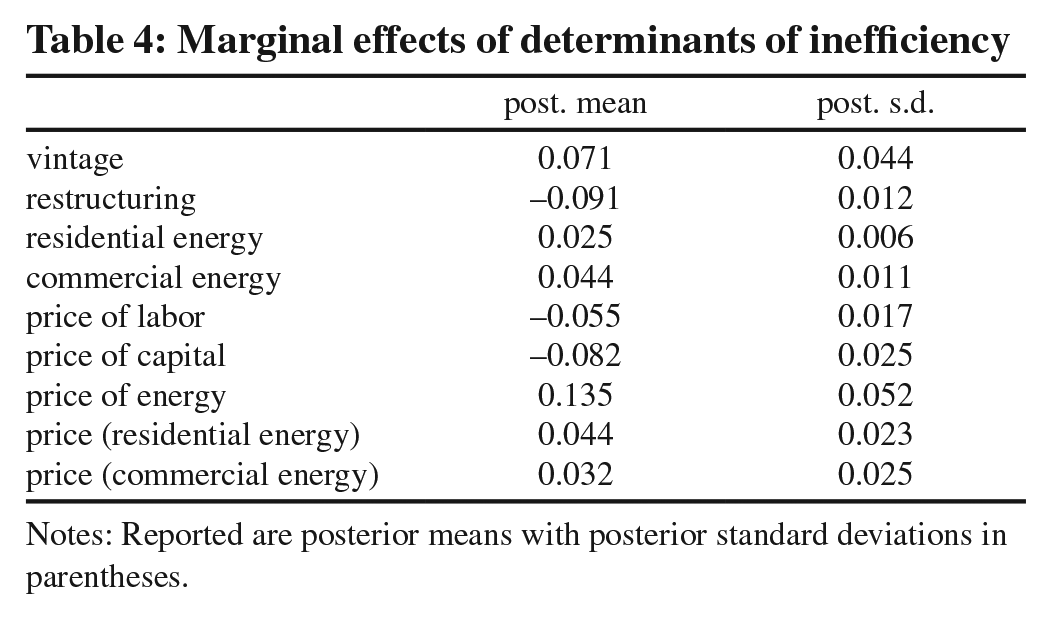
Notes: Reported are posterior means with posterior standard deviations in parentheses.

Sampling distributions of some of these marginal effects are presented in Figure 4. It can be seen that the marginal effects of bad outputs on inefficiency are negative. These plots indicate that utilities that produce more bad outputs are also more inefficient. These findings suggest that plants that produce more bad outputs have poor management quality which is showing up in high inefficiency.

Figure 4

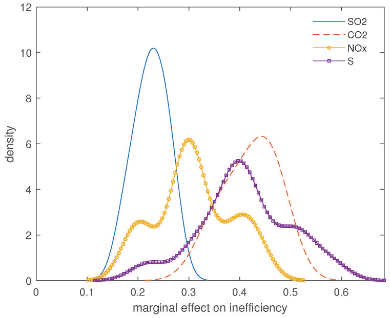
Marginal effects of bad outputs on inefficiency

4.5 Dynamic effects

The dynamic effect of $Z_{t}$ and $B_{t}$ on inefficiency can be obtained by taking partial derivatives of $s_{t} = ρ_{1} W s_{t} + ρ_{2} W s_{t - 1} + Z_{t} γ + B_{t} ω + ξ_{t 1}$ (which is equation (4)). In Figure 5, we show the dynamic effect of inefficiency on the numeraire input labor. Since the IDF is homogeneous of degree one in inputs, we can interpret the marginal effect as the percentage increase in cost die to inefficiency. Panel (a) of Figure 5 shows that the percentage change in cost due to inefficiency has decreased steadily over time from a little above 90% to 43%. In panels (b) and (c) we report the direct (own) percentage contribution and indirect (due to others). Panel (b) shows that the own percentage effect decreased over time, while the percentage contribution due to other increased from 10% to 58%.

Figure 5

Dynamic effect of inefficiency on cost (%)

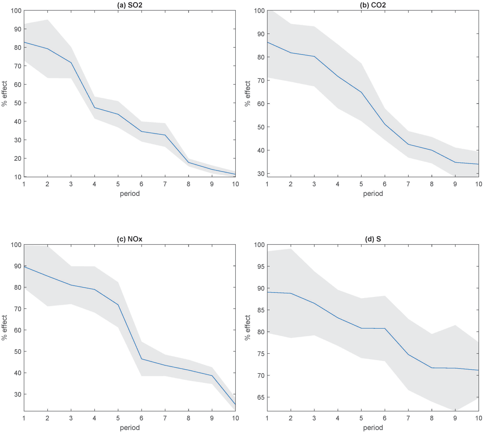
In panels (a) through (d) of Figure 6, we report dynamic effects of bad outputs on inefficiency; specifically their percentage contribution to own production of bad outputs. This is computed using the simultaneous relationship between bad outputs and good output. That is, $\partial u_{t} / \partial B_{tj} = \partial u_{t} / \partial Y_{t} \times \partial Y_{t} / \partial B_{tj}$ , where the first part comes from (9).

Figure 6

Dynamic effects of bad outputs on inefficiency

4.6 Output elasticities

Finally, in Table 5, we report posterior moments for certain elasticities. Note that elasticity of $x_{1}$ with respect to $Y_{1}$ and $Y$ can be interpreted as cost elasticity sum of which is the reciprocal of returns to scale (RTS). Thus at the mean we have $RTS = 1 / (0.651 + 0.372) = 0.977$ , which is not much different from 1 both economically and statistically. We interpret the elasticities of $x_{1}$ with respect of bad outputs as the shadow prices of different types of pollutants. These are all negative as expected because an increase (decrease) in pollutants gives plants a cost advantage in disposing the pollutants freely, and they range from –0.137% to –0.36%. In other words, plats have to incur additional costs to reduce their bad outputs.⁵ In Table 5 we report the elasticities instead of their partial derivatives. The elasticities in the second block of the table come from the bad output technologies in equation (7) or (9). These indicate societal cost of increasing the good outputs, and are expected to be positive. Since there are spatial effects on these, we report the overall elasticities in column 2. Interestingly, spillover effects account for the majority of the total effect, indicating that neighborhood effects are more important than own effects. That means, the neighboring plants seems to play a crucial role indicating “contagion” of practices.

Table 5

Marginal effects (elasticities)

	post. mean (post. s.d.)	% own
∂ logx₁/∂ logY₁	0.651	—
	(0.037)	—
∂ logx₁/∂ logY₂	0.372	—
	(0.045)	—
∂ logx₁/∂ logB₁	0.137	—
	(0.045)	—
∂ logx1/∂ logB2	0.251	—
	(0.059)	—
∂ logx₁/∂ logB₃	0.288	—
	(0.076)	—
∂ logx₁/∂ logB₄	0.360	—
	(0.085)	—
∂ logB₁/∂ logY₁	0.215	34.67%
	(0.071)	(7.44%)
∂ logB₁/∂ logY₂	0.415	32/17%
	(0.065)	(9.44%)
∂ logB₂/∂ logY₁	0.127	25.44%
	(0.032)	(7.81%)
∂ logB₂/∂ logY₂	0.315	32.51%
	(0.045)	(12.44%)
∂ logB₃/∂ logY₁	0.355	16.32%
	(0.083)	(4.55%)
∂ logB₃/∂ logY₂	0.250	28.25%
	(0.056)	(6.92%)
∂ logB₄/∂ logY₁	0.313	35.44%
	(0.107)	(7.39%)
∂ logB₄/∂ logY₂	0.503	27.32%
	(0.029)	(5.45%)
∂ logu/∂ logB₁	0.225	32.37%
	(0.031)	(7.34%)
∂ logu/∂ logB₂	0.420	28.44%
	(0.049)	(9.32%)
∂ logu/∂ logB₃	0.310	22.55%
	(0.075)	(6.70%)
∂ logu/∂ logB₄	0.410	36.55%
	(0.091)	(7.43%)

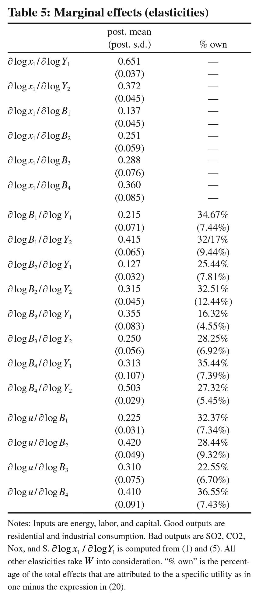
Notes: Inputs are energy, labor, and capital. Good outputs are residential and industrial consumption. Bad outputs are SO2, CO2, Nox, and S. ∂ logx₁/∂ logY₁ is computed from (1) and (5). All other elasticities take W into consideration. “% own” is the percentage of the total effects that are attributed to the a specific utility as in one minus the expression in (20).

In the last block of the table we report the marginal effects (elasticities) of bad outputs on inefficiency. As mentioned earlier, these effects are all positive indicating that an increase in bad output is associated with an increase in inefficiency (and therefore cost). This might the effect of tight regulation meaning that when plants an increase bad outputs is not free—plants need to incur additional cost by buying permits to pollute, for example. Alternatively, when bad outputs increase, more management (quality) is exercised as the production of bad outputs is highly regulated in the U.S.⁶

5. Concluding Remarks

In this paper we use a bi-production approach to model production of good and bad outputs. The good output production technology is modeled using an input distance function. We use panel data on the U.S. electric utilities for this. In the production of good outputs we allow for the endogeneity of inputs and bad outputs (SO2, CO2, NOx and S). This enables us to estimate the marginal effect of an increase in good output on the production of each bad ouput. The shadow prices, on the other hand, indicate the sacrifice of good output for a decrease in the production of each bad output. Thus, conceptually it is the opposite of the marginal effects of good output, and is associated with a decrease in each of the bad output. The shadow elasticities in a logarithmic model is the percentage decrease (sacrifice) in good output for a one percent decrease in each bad output due to a 1% increase in good output. In our proposed model the elasticities of each of the bad outputs are directly estimated, instead of the shadow elasticities. These elasticities range from 0.137% to 0.36%. An advantage of using the IDF is that since $\partial 1 n x_{1} / \partial 1 n B_{m} = \partial 1 n x_{1} / \partial 1 n Y_{1} \div \partial 1 n B_{m} / \partial 1 n Y$ , estimated cost elasticity of each bad output is related to cost elasticity of good output and shadow elasticities in a unique way. The elasticities are reported in Table 5. Technical inefficiency is assumed to follow a spatial dynamics process to examine the spatial effects in inefficiency in the production of good outputs. Consequently, the model allows us to compute the direct, indirect and overall effect of its determinants. Table 5 reports these effects for the bad outputs. We also model production of each bad output with a spatial structure—each depending on production of good outputs, inputs and other exogenous variables. These bad output production functions allow us to estimate both direct and indirect effects of good outputs, which may be of special interest because they show the cost (to the society) in terms of releasing pollutants to the environment in order to increase production of good outputs. We apply the new technique to a panel data on U.S. electric utilities with four bad outputs, three inputs and two good outputs. We find returns to scale close to unity. Bad outputs are found to affect positively to inefficiency. Percentage increases in inefficiency due to a percentage increase in each bad output are found to vary from 0.225% to 0.42%. Vintage of the plant is found to increase inefficiency while restructuring decreased inefficiency. Energy prices are found to be positively related to inefficiency. From the SAR specifications of bad outputs, we find that the spillover effects of (the societal cost) increasing the good outputs account for the majority of the total effect, indicating that neighborhood effects are more important than own effects. The percentage of own effects range from 16.32% to 35.44%. This means, the neighboring utilities played a crucial role indicating “contagion” of practices.

Supplemental Material

sj-pdf-1-enj-10.5547_01956574.45.1.mtsi – Supplemental material for Endogenous Bad Outputs and Technical Inefficiency in U.S. Electric Utilities

Supplemental material, sj-pdf-1-enj-10.5547_01956574.45.1.mtsi for Endogenous Bad Outputs and Technical Inefficiency in U.S. Electric Utilities by Mike Tsionas and Subal C. Kumbhakar in The Energy Journal

Footnotes

Appendix A

Appendix B

First, we focus on sensitivity of the posterior with respect to our prior assumptions. In our benchmark prior, we have $\bar{N} = 1$ , $\bar{a} = 1$ , and $h = 10$ . We generate 1,000 different priors by assigning 1,000 different values to the prior parameters as follows.

The results are reported in Figure B.1 for the main quantities of interest, viz. productivity growth (panel (a)), inefficiency (panel (b)), IDF parameters (panel (c)) and reduced form parameters for both inputs and bad outputs in panel (d)). Across the 10,000 different priors, reported are densities of differences of posterior means and posterior standard deviations relative to the benchmark case.⁷ Evidently, the model is reasonably robust so, inferences based on the benchmark prior are representative.

To examine numerical performance we rely on autocorrelation functions (panel (a) of Figure B.2), and the standard Geweke (1992) diagnostics, viz. relative numerical efficiency (RNE, panel (b)), and convergence diagnostics (GCD, panel (c)). We consider acfs, RNEs and absolute GCDs for a given lag across 50 randomly chosen parameters. RNE should be close to one if i.i.d sampling from the posterior were possible and GCDs follow asymptotically (in the number of MCMC draws) a standard normal distribution so, deviations from 1.96 would indicate non-convergence. Specifically, GCD is the absolute value of a a z-test that compares the first and last 25% of means of MCMC draws. For PF methods to be effective, the weights should be approximately uniformly distributed to avoid a degenerate situation where just a few particles have a weight close to 1 and the vast majority of others are zero. In panel (d) we show 50 representative particle weights corresponding to our state variables. These results indicate that although the weights are not uniformly distributed they do not have degenerate distributions either. Finally, in panel (e) we report acfs for inefficiency estimates across fifty randomly selected is and ts. For other is and ts the behavior of acfs was qualitatively the same. From these results it turns out that MCMC mixes well and allows a thorough exploration of the posterior.

Appendix C

To examine the role of instruments, we report the distribution on R-squared from (5) and (7) across MCMC iterations, which will provide evidence on the strength of instruments. Our results are reported in panel (a) of Figure C.1. Second, we report correlation coefficients from the first row of ∑ corresponding to (1). These are reported in panel (b) of Figure C.1. From this evidence, we can claim that the instruments are strong and valid.

1.

Although shadow prices are calculated in Färe et al. (2005), , their models do not control for endogeneity of bad outputs. Consequently, the estimates are likely to be biased and inconsistent.

2.

Similarly, there some other papers in the SF literature that deal with endogeneity of inputs. For example, Tsionas et al. (2015), use an IDF system approach without no bad outputs. These papers are not important to discuss here because none of them, to the best of our knowledge, discuss endogeneity in the context of a bi-production model. With or without endogeneity of inputs, the bi-production models constitute a system as in KT.

3.

We assume that the variables in $f (Y_{t}; β)$ appear in logarithms and $x_{t 1}$ is log of the normalizing input.

4.

We assume W is row normalized and all spatial autoregressive parameters are non-negative and less than one. See .

5.

In a cost function, these shadow prices are partial derivatives of cost with respect to bad outputs with a negative sign. Since the IDF is dual to the cost function, we expect to find similar results.

6.

We have not formally introduced management in the bad output production functions.

7.

We make use of the sampling-importance-resampling algorithm of Rubin (1987, 1998); see also .

References

Agee

Atkinson

Crocker

Williams

(2014). “Non-separable pollution control: Implications for a CO2 emissions cap and trade system.” Resource and Energy Economics 36: 64–82. https://doi.org/10.1016/j.reseneeco.2013.11.002.

Andrieu

Doucet

Holenstein

(2010). “Particle Markov chain Monte Carlo methods (with discussion).” Journal of the Royal Statistical Society Series B 72(2): 1–33. https://doi.org/10.1111/j.1467-9868.2009.00736.x.

Atkinson

S.E.

Tsionas

M.G.

(2018). “Shadow directional distance functions with bads: GMM estimation of optimal directions and efficiencies.” Empirical Economics 54: 207–230. https://doi.org/10.1007/s00181-017-1233-6.

Atkinson

S.E.

Primont

Tsionas

M.G.

(2018). “Statistical inference in efficient production with bad inputs and outputs using latent prices and optimal directions.” Journal of Econometrics 204(2): 131–146. https://doi.org/10.1016/j.jeconom.2017.12.009.

Atkinson

Primont

Tsionas

M.G.

Atkinson

Dorfman

(2005). “Bayesian measurement of productivity and efficiency in the presence of undesirable outputs: crediting electric utilities for reducing air pollution.” Journal of Econometrics 126: 445–468. https://doi.org/10.1016/j.jeconom.2004.05.009.

Bigerna

D’Errico

M.C.

Polinori

(2019). “Environmental and energy efficiency analysis of EU electricity industry: An almost spatial two stages DEA approach.” The Energy Journal 40: 31–56. https://doi.org/10.5547/01956574.40.1.sbig.

Bigerna

D’Errico

M.C.

Polinori

(2020). “Heterogeneous impacts of regulatory policy stringency on the EU electricity Industry: A Bayesian shrinkage dynamic analysis.” Energy Policy 142. https://doi.org/10.1016/j.enpol.2020.111522.

Chopin

Singh

S.S

(2013). “On the particle Gibbs sampler.” Working paper, ENSAE. http://arxiv.org/abs/1304.1887.

10.

Creal

D.D.

(2012). “A survey of sequential Monte Carlo methods for economics and finance.” Econometric Reviews 31(3): 245–296. https://doi.org/10.1080/07474938.2011.607333.

11.

Creal

Tsay

(2015). “High dimensional dynamic stochastic copula models.” Journal of Econometrics 189(2): 335–345. https://doi.org/10.1016/j.jeconom.2015.03.027.

12.

DiCiccio

T.J.

Kass

R.E.

Raftery

Wasserman

(1997). “Computing Bayes Factors by Combining Simulation and Asymptotic Approximations.” Journal of the American Statistical Association 92(439): 903–915. https://doi.org/10.1080/01621459.1997.10474045.

13.

Färe

Grosskopf

Noh

D.W.

Weber

(2005). “Characteristics of a polluting technology: theory and practice.” Journal of Econometrics 126: 469–492. https://doi.org/10.1016/j.jeconom.2004.05.010.

14.

Fernández

Koop

Steel

M.F.J.

(2002). “Multiple-Output production with undesirable outputs: an application to nitrogen surplus in agriculture.” Journal of American Statistical Association 97: 432–442. https://doi.org/10.1198/016214502760046989.

15.

Førsund

F.R.

(2009). “Good Modelling of Bad Outputs: Pollution and Multiple-Output Production.” International Review of Environmental and Resource Economics 3(1): 1–38. https://doi.org/10.1561/101.00000021.

16.

Geweke

(1992). “Evaluating the Accuracy of Sampling-Based Approaches to the Calculation of Posterior Moments,” In: Bernardo

J. M.

Berger

J. O.

Dawid

A.P.

Smith

A.F.M.

Eds., Bayesian Statistics, Vol. 4, Clarendon Press, Oxford: 169–193. https://doi.org/10.21034/sr.148.

17.

Girolami

Calderhead

(2011). “Riemann manifold Langevin and Hamiltonian Monte Carlo methods.” Journal of the Royal Statistical Society Series B 73 (2): 123–214. https://doi.org/10.1111/j.1467-9868.2010.00765.x.

18.

Godsill

S.J.

Doucet

West

A.M.

(2004). “Monte Carlo smoothing for nonlinear time series.” Journal of the American Statistical Association 99(465): 156–168. https://doi.org/10.1198/016214504000000151.

19.

Kass

R.E.

Raftery

A.E.

(1995). “Bayes factors.” Journal of the American Statistical Association 90(430): 773–795. https://doi.org/10.1080/01621459.1995.10476572.

20.

Koop

Pesaran

M.H.

Potter

(1996). “Impulse Response Analysis in Nonlinear Multivariate Models.” Journal of Econometrics 74: 119–147. https://doi.org/10.1016/0304-4076(95)01753-4.

21.

Kumbhakar

S.C.

(2013). “Specification and estimation of multiple output technologies: A primal approach.” European Journal of Operational Research 231: 465–473. https://doi.org/10.1016/j.ejor.2013.05.019.

22.

Kumbhakar

S.C.

Tsionas

(2016). “The good, the bad and the technology: Endogeneity in environmental production models.” Journal of Econometrics 190: 315–327. https://doi.org/10.1016/j.jeconom.2015.06.008.

23.

Kutlu

(2018). “Estimating efficiency in a spatial autoregressive stochastic frontier model.” Economics Letters 163: 155157. https://doi.org/10.1016/j.econlet.2017.12.025.

24.

Murty

Russell

Robert

Levko

S.B.

(2012). “On modeling pollution-generating technologies.” Journal of Environmental Economics and Management 64(1): 117–135. https://doi.org/10.1016/j.jeem.2012.02.005.

25.

Pesaran

M.H.

Shin

(1998). “Generalized Impulse Response Analysis in Linear Multivariate Models.” Economics Letters 58: 1729. https://doi.org/10.1016/S0165-1765(97)00214-0.

26.

Rubin

D.B.

(1987). “A noniterative sampling-importance resampling alternative to the data augmentation algorithm for creating a few imputations when fractions of missing information are modest: The SIR algorithm.” Journal of the American Statistical Association 82: 543–546. https://doi.org/10.2307/2289460.

27.

Rubin

D.B.

(1988). “Using the SIR algorithm to simulate posterior distributions.” In Bayesian Statistics 3, ed. Bernardo

J.M.

DeGroot

M.H.

Lindley

D.V.

Smith

A.F.M.

, 395–402.

28.

Smith

A.F.M.

Gelfand

(1992). “Bayesian statistics without tears: A sampling resampling perspective.” The American Statistician 46: 84–88. https://doi.org/10.1080/00031305.1992.10475856.

29.

Tierney

(1994). “Markov chains for exploring posterior distributions.” The Annals of Statistics 1701–1728. https://doi.org/10.1214/aos/1176325750.

30.

Tsionas

M.G.

(2006). “Inference in dynamic stochastic frontier models.” Journal of applied econometrics 21: 669–676. https://doi.org/10.1002/jae.862.

31.

Zellner

(1971). An introduction to Bayesian inference in econometrics. Wiley, New York.

Supplementary Material

Please find the following supplemental material available below.

For Open Access articles published under a Creative Commons License, all supplemental material carries the same license as the article it is associated with.

For non-Open Access articles published, all supplemental material carries a non-exclusive license, and permission requests for re-use of supplemental material or any part of supplemental material shall be sent directly to the copyright owner as specified in the copyright notice associated with the article.

0.00 MB

0.04 MB