Retail Electricity Market Restructuring and Retail Rates

Abstract

Prior to the 1990s, all U.S. states used a “cost of service (COS)” regulation regime in which investor-owned utilities were allowed to recover prudently incurred costs plus a rate of return on capital expenditures, and retail customers were unable to choose their electricity supplier. From 1996–2000, multiple states passed retail electricity market “restructuring.” This empirical research examines the effect of retail restructuring on electricity prices to final consumers. We find that rates increased in restructured states relative to plausible counterfactuals in the years post-restructuring. But by twelve years after retail restructuring, we no longer observe any difference. We investigate plausible mechanisms, finding evidence that retail prices became more responsive to natural gas prices due to retail restructuring, the timing of which coincided with increases in natural gas prices nationally. We also test for whether restructuring had distributional effects across customer classes and find that in the short run residential customers benefited relative to industrial customers during transition periods, but that this difference does not persist into full implementation.

1. Introduction

Electric utilities are a classic example of a natural monopoly in which regulators—in lieu of markets—set rates (i.e. prices). ¹ In the United States, investor-owned utilities are regulated on a state-by-state basis and these regulatory regimes differ substantially. Prior to the 1990s, states typically used a “cost of service” (COS) regulatory regime, where utilities recover prudently incurred costs plus a rate of return. Regulators set the rate of return to allow utilities to attract investment capital needed for up-front investments and recover these costs over years from ratepayers. ²

In the late 1990s, a number of states changed their traditional regulatory approach, and began implementing electricity market “restructuring” (sometimes referred to as “deregulation” colloquially and in the literature). Retail restructuring reforms at the state level typically targeted generation ownership and remuneration as well as the reform of retail services to allow consumers to choose an alternate supplier of electricity. State-level reforms often required the separation of generation function, thus transitioning the generation capacity from COS to market-based remuneration while also requiring incumbent utilities that unbundled their rates to divest their generation plants to either an affiliate or unrelated entity. States also required competition in the retail sector, allowing third-party, energy-only retailers to buy power in the wholesale market and sell to end-use customers (Borenstein and Bushnell, 2015). Competition in the retail sector was referred to in many ways, including retail restructuring, retail access, or retail choice.

In some states, regulators began allowing customers to contract with non-utility power generators for their electric supply, in essence circumventing the incumbent utility. ³ The most famous example of retail restructuring occurred in California, which underwent an electricity market crisis in 2000–2001. Companies such as Enron were blamed for this crisis due to exploitation of the specific rules of the state’s restructuring legislation to influence market prices to their advantage. But not all states that underwent retail restructuring experienced such results and fourteen states that implemented restructuring in the early 2000s maintain this regulatory structure today. As shown in Map 1, state level restructuring was concentrated in the Northeast and Western United States, with the notable exception of Texas in the South. Several of the states in the West either reversed or implemented hybrid policies plausibly spurred by California’s energy crisis. Altogether, wholesale and retail restructuring of the U.S. electric power industry has been described as one of the largest single industrial reorganizations in the history of the world (Kwoka, 2008). ⁴

Recently, renewed attention has been given to retail access in the aftermath of the 2021 Texas power crisis. In February of 2021, three severe winter storms swept across Texas, leading simultaneously to historic levels of demand and the failure of a number of large generating stations. In response, the Electric Reliability Council of Texas (ERCOT) set the wholesale market price of electricity at its cap of $9,000 per MWh for approximately four days. Interestingly, facilitated by retail choice in Texas, some rate plans allow customers, including less sophisticated residential customers, to pay the wholesale price for electricity plus some markup. ⁵ Assuming average usage, this would amount to an over $1,400 electricity bill for a residential customer for just four days. ⁶ This is perhaps a dramatic example of how retail access could create sharp temporary price increases for a final use customer. ⁷ Electricity market design has been at the center of the debate of the cause of the Texas power crisis. Thus, although the most recent jurisdiction to pass retail restructuring was more than two decades ago (Washington DC in 2000), implications are relevant to policy makers to this day.

Map 1:

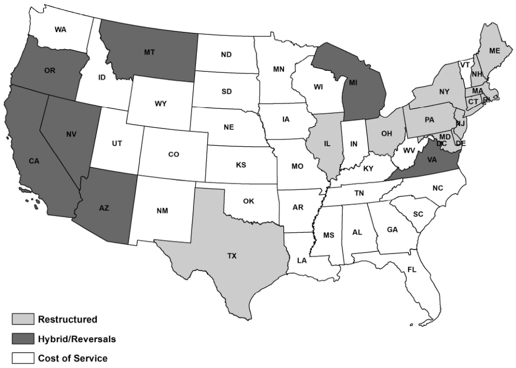
Map of State-level Restructuring Policies

We examine the effect of retail restructuring on end-use or retail customer rates and focus on state-level electricity market restructuring reforms that enabled retail competition, not the development of RTO markets explicitly. ⁸ Specifically, we conduct three empirical tests, all utilizing a differences-in-differences research design. First, we will test for the effect of retail restructuring on prices by customer class. Second, we will consider how retail restructuring affected relative prices across customer classes, namely commercial and industrial relative to residential rates. Last, we will examine the relationship between retail rates (by customer class) and natural gas prices within restructured and non-restructured states to examine if prices are more responsive to fuel price changes in retail-restructured states. We also implement an event study style analysis to both test the parallel pre-trends assumption and examine the timing of any observed impact. Standard robustness checks such as placebo tests, diagnostics of and robust inference of parallel trends tests, and tests for other cofounding outcomes that could reveal threats to identification are also conducted. We will also address recent methodological critiques of the two-way fixed effects difference-in-differences approaches with variation in treatment timing (Goodman-Bacon, 2019; Sun and Abraham, 2021) by employing a stacked regression robustness similar to Cengiz et al. (2019).

Importantly, and novel to this research, all empirical analyses are based on detailed descriptions of each state’s restructuring timeline, including its transition period and date of full retail-restructuring implementation. Properly identifying restructuring states and dates has been a common critique of this literature, which we address seriously in this analysis. We carefully research each state that passed restructuring legislation to understand the date that restructuring began. Following the start of retail restructuring, we allow for a transition phase. This phase starts with the opening of a competitive retail market. We define this phase as a transition because discounts and rate freezes were typical for customers transitioning to market prices. Following the transition phase, we then define the date that full retail market access was attained for each retail restructured state. This phase is characterized by customers paying market-based prices by either choosing their own supplier or through some aggregation mechanism. ⁹ To summarize, we consider treatment effects for (1) all restructured states post-restructuring inception, (2) transition period, and (3) post-full retail market access attainment. To see the importance of considering these different phases of restructuring, four states took ten or more years from the beginning to end of restructuring implementation; the median state took seven years. Importantly, we also exclude hybrid states and states that later reversed policies from both treatment and control groups, although we provide a supplemental analysis of these states in the Online Appendix. We will show that properly identifying treatment areas and timing has important implications for the results. We hope that this will benefit future work aiming to properly identify state level policy changes.

This research will also consider plausibly non-random policy adoption and how this might bias empirical observations. To do so, we first present a “naïve” approach that simply estimates the actual retail-price change in restructured and non-restructured states after restructuring took place (i.e. standard difference-in-differences). This baseline estimate does not account for endogenous policy adoption. Next, we present results using a synthetic control analysis (Abadie, Diamond, Hainmueller, 2010; Abadie 2021) that compares electricity rates in restructured states relative to non-restructured states with similar economic, political, and electricity market characteristics ex ante to provide a more plausible counterfactual. Comparison of these two approaches provides insight into whether non-random policy adoption is important in interpreting non-causal observations from prior literature.

Also important, the time period of analysis extends from 1990 to 2019. Due to the long lag time from when states passed laws, began the restructuring process, and implemented full retail market access, this time period of almost three decades is necessary. While all states had passed restructuring legislation by 2000, the median year that full retail market access was available was 2007, with the most recent completion occurring in Pennsylvania in 2012. ¹⁰ Early studies of restructuring’s effect on retail electricity markets could not include any time observations post-full retail restructuring implementation—our study overcomes this limitation. ¹¹

We argue that this is altogether the most comprehensive analysis of state level restructuring policies, arguably the largest state level change in electricity markets in the United States over the past half century. This is the first analysis to consider non-random adoption utilizing ex ante state level characteristics. A randomized control trial is unavailable in this context, and we can therefore not rule out the possibility of a form of unobserved heterogeneity that would preclude results from being interpreted as causal, although this is a challenge for inference utilizing state level policies more broadly.

The remainder of the paper will move forward as if the reader is familiar with the history and structure of the electric utility industry in the United States broadly and retail competition policies specifically. A background of relevant information on the U.S. electricity regulation and its history is provided in Appendix B.

1.1 Conceptual Framework

Although our contribution is empirical, not theoretical, we motivate our empirical questions in prevailing theory. An extended discussion of the prevailing theory is provided in Appendix C.

In states with a COS regulatory regime, utilities recover prudently incurred costs plus an allowed rate of return on capital. If the rate of return allowed by the regulator is too high, a monopoly with COS-based rates has an incentive to overcapitalize (Averch & Johnson, 1962)—known as “gold plating” or the “A-J effect” (Knittel et al., 2019).

As discussed in Appendix C, if the allowed rate of return is too high, retail restructuring has two potential effects: (1) moving to a less capital-intensive production process can create efficiency gains, (2) moving the price closer to the competitive market price can transfer welfare from producers (i.e. utilities) to consumers (i.e. ratepayers). However, economic gains from retail restructuring might not be possible (or undetectable empirically) if state regulators had effectively set the allowed rate of return equal to the market cost of capital. Whether retail restructuring is effective at reducing electricity rates paid by customers is the first empirical question addressed in this research.

A second implication of the A-J model is that a firm has an incentive to enter into other markets—even if the cost of doing so exceeds revenues in the long run—because expanding into other markets enables the firm to inflate its capital expenditures and increase overall profits. Known as the “multi-market” case, it implies that one market is used to subsidize the other and might also be applicable to customer rate classes in this context.

When a regulator establishes rates across customer classes, the share of the costs incurred in serving each class (residential, commercial and industrial customers) is important. Consider ${\mathrm{\gamma }}_c$ as the true value of the share of costs associated with customer class c where ${\sum }_c{\gamma }_c=1$ . In words, the share of costs allocated all rate classes sums to one. Consider ${\widehat{\gamma }}_c$ as the regulator’s estimate of ${\mathrm{\gamma }}_c$ for each customer class. ¹² ${\widehat{\gamma }}_c={\mathrm{\gamma }}_c\forall c,$ If regulators are successful in setting, then there will not be cross subsidization across customer classes. But in the case where ${\widehat{\gamma }}_c\ne {\mathrm{\gamma }}_c\forall c,$ one customer class will subsidize another. For example, regulators typically allocate a larger share of costs to residential customers to account for the investment required to distribute electricity to many individual customers, whereas industrial customers—who purchase larger quantities of electricity—impose lower costs per kWh on the utility. If the residential customer class accounts for an even larger share of the cost than set by the regulator, ${\widehat{\gamma }}_{res}<{\mathrm{\gamma }}_{res},$ , it is possible that industrial customers might subsidize residential customers even if the industrial electricity rate is lower. The converse is also possible. Because regulators are appointed (or elected) through political processes, critiques of COS based regulation have claimed that these relative rates can also be influenced by political factors.

If retail restructuring is implemented and a customer can now procure power from a third party, two things might happen. First, in a competitive market, customers in a class paying a proportionally larger share of costs will be incentivized to procure lower-cost power from a different supplier. Second, the restructured utility may then have an incentive to set ${\widehat{\gamma }}_c={\mathrm{\gamma }}_c$ to reduce customers’ incentives to obtain power from another seller. In this way, retail restructuring might reduce cross-subsidization between rate classes, therefore changing relative rates between classes. Whether retail restructuring changed relative rates between customer classes is the second empirical question addressed in this research.

The extent to which retail market restructuring has increased the response of electricity prices to fuel costs is the third empirical question addressed in this research. A number of studies have investigated fuel costs pass through to retail rates, finding mixed results (Whitworth and Zarnikau, 2006; Knittel et al. 2019; Ohler et al. 2020). ¹³

Also pertinent to our empirical analysis, during periods in which rates in restructured and COS states diverge, due to differences in rate design or by economic factors outside of the regulatory structure, political sentiment might tilt towards whichever regime (COS or restructuring) might offer the lowest price at that time (Borenstein & Bushnell, 2015). Our synthetic control approach will address this by comparing restructured states to a weighted average of COS states with similar economic, political, and electricity market characteristics ex ante.

1.2 Literature

We present a concise review of the literature on electricity market restructuring. While we present six broad categories of research, our research specifically addresses the first three, namely, the impact on retail prices, cross-subsidization across customer classes, and fuel cost pass-through to rates. Although prior research has examined retail electricity market restructuring in different countries (e.g. Ganev, 2009; Pineau & Hämäläinen, 2000; Outhred, 1998), this literature review will largely focus on U.S. electricity markets.

1.2.1 Retail Restructuring and Retail Prices

To date, the literature on restructuring’s impact on retail rates has been mixed. Joskow (2006), Swadley & Yucel (2011), Su (2015), Ros (2017), and Hartley et al. (2019) find that restructuring led, in some instances, to decreases in electricity prices for final customers, while Showalter (2007), Tierney (2007), and Borenstein & Bushnell (2015) all point out that electricity prices actually increased in restructured states relative to COS states after restructuring.

Borenstein & Bushnell (2015), which provides a comprehensive review of the U.S. electricity industry, observes (consistent with this research) that prices increase in regions with restructuring post restructuring, and that this increase is coincident with natural gas price increases. But the review article explicitly highlights that this observation is not intended to be an exhaustive analysis of the drivers of retail prices and cites prior analyses that utilize data during the early years of retail restructuring (Apt 2005; Taber et al. 2006). Our analysis aims to fill this gap in the literature called for in this review article. Hartley et al. (2019) also observe a similar pattern juxtaposing restructured vs. non-restructured regions within Texas, but do not consider effects across states.

1.2.2 Cross-Subsidization across Customer Classes

Several studies also focus on the potential for cross-subsidization across rate classes and potential implications of retail restructuring policies on class cross-subsidization. Using micro-data from customer bills, Dormady et al. (2019) find that retail restructuring has shifted the financial burden towards residential customers in Ohio. Nagayama (2007) and Erdogdu (2011) consider cross-subsidization but focus on a panel of countries, in lieu of U.S. states as is the focus of this analysis. Nagayama (2007) find that there was a tendency for prices to rise, while Erdogu (2011) findings imply that reform had different impacts in different countries, which supports the idea reform prescription for a specific country cannot easily and successfully be transferred to another.

1.2.3 Fuel Cost Pass-Throughs

Knittel et al. (2019) find that electric power producers were more responsive to fuel prices in vertically integrated markets than in restructured markets but does not conduct similar tests for prices paid by customers. Results from Ohler et al. (2020), on the other hand, do not support the view that restructuring increased the integration between input costs and electricity prices.

Hartley, Medlock & Jankovska (2019) utilize bill data from Texas finding that residential customers benefited from retail choice and note that these benefits were likely facilitated by the fall in natural gas prices that occurred post restructuring in Texas. ¹⁴ In other words, it was the pass-through of generation costs facilitated by restructuring that allowed customers to reap the benefits of lower natural gas prices. Whitworth and Zarnikau (2006), also focusing on Texas, reached a similar conclusion regarding natural gas fuel cost pass-through to restructured regions.

1.2.4 Generation Plant Level Efficiency

A related literature on plant-level efficiency also finds mixed results in restructured regions relative to COS regions. For example, some studies find no improvements in fuel (thermal) efficiency (Fabrizio et al. 2007; Knittel et al. 2019), while others find small but significant thermal efficiency improvements in restructured regions (Bushnell & Wolfram, 2005; Zhang, 2007; Sharabaroff et al., 2009; Craig & Savage, 2013; Chan et al., 2017; Doyle & Fell, 2018). ¹⁵ Efficiency improvements are not explicitly considered in this analysis, but if present these plant level efficiency improvements could pass through to ratepayers in the form of bill savings.

1.2.5 Regional Transmission Organizations

While not the specific focus of this research, the creation of regional transmission organizations (RTOs) ¹⁶ in the restructuring era has been shown to reduce transmission congestion externalities (Kleit & Reitzes, 2008; Wolak, 2011; Mansur & White, 2012) and create gains from trade due to better matching of buyers and sellers (Mansur & White, 2012; Kury, 2015). Kury (2013) finds that only fully restructured states experienced significant retail price decreases in RTO regions.

In contrast to wholesale restructuring’s transmission benefits, the literature on overall wholesale market performance finds that market power persists in the short run in RTO electricity markets (Borenstein, 2002; Borenstein et al., 2002; Joskow & Kahn, 2002; Wolak, 2003; Bushnell, 2004; Puller, 2007; Bushnell et al., 2008; Hortacsu & Puller, 2008; Mansur, 2008). Structural characteristics of electricity markets—supply constraints in peak conditions and inelastic demand—can lead to the exercise of horizontal market power, resulting in higher prices than found in purely competitive markets. In the event that market power is exacerbated by restructuring, this could increase rates for customers and shift rents towards utilities.

1.2.6 Endogenous Policy Adoption

Prior academic literature has tested for the non-random adoption of retail electricity market restructuring, finding electricity prices and political influence are predictive of restructuring (Craig, 2016). ¹⁷ Related literature on renewables portfolio standards (RPSs) has also shown that political and economic factors can impact a state’s decision to implement statewide electricity market policies (Ming-Yuan et al., 2007; Chandler, 2009; Lyon and Yin, 2010; Fowler and Breen, 2013; Upton and Snyder, 2015) and that taking this non-random adoption into account has important impacts on empirical results (Upton & Snyder, 2017). For this reason, we will consider variables known to impact policy adoption in creation of our synthetic control analysis.

2. Data

We utilize a panel of 48 continental states plus Washington DC from 1990 to 2019. ¹⁸ Ideally, we would like to be able to consider utilities in lieu of states, but this is not possible given the constraints of the data. ¹⁹ Outcome variables include state-level average electricity prices by customer type including residential, commercial, and industrial customers (U.S. Energy Information Administration (EIA)). ²⁰ Synthetic control groups are constructed using data on the number of members of state house and senate by political party, the political party of the governor, gross state product, mining and manufacturing gross state product, the share of industrial and commercial customers and the percent of generation capacity within the state that comes from natural gas. ²¹ State-level renewable energy generation and gasoline consumption are used as additional outcome variables to address whether potentially cofounding factors can preclude results from being interpreted as causal. State-level population is used to normalize many of these variables for appropriate cross-state comparisons. See Abadie (2021) for a synopsis of synthetic control analysis.

The variables used to construct synthetic controls were collected from four sources. Political data on the number of Democrats and Republicans in each state’s legislature and the party of the governor were collected from Klarner (2019). For all statistical results, the Democratic members of both the House and the Senate as a percent of the total members of both bodies are used. Data on the gross state product and the mining and manufacturing gross state products were collected from the U.S. Bureau of Economic Analysis. ²² The share of load consumed by commercial and industrial customers (Form 861) and the generating capacity share from natural gas (Form 860) are from the EIA.

We utilized the EIA’s state-level estimates of renewable energy generation (kWh) from all major renewable energy sources including geothermal, biomass, solar thermal and photovoltaic, wind and wood derived fuels. ²³ While the main purpose of retail restructuring policies was not increasing renewable energy penetration, this is a testable hypothesis.

We will also utilize data on cooling degree days (CDDs), computed by the National Weather Service’s Climate Prediction Center. CDDs are the positive differences in the mean temperature above a 65°F base. For example, if a mean temperature of 68°F is recorded on a given day, that day would be recorded as three CDDs. The annual number of CDDs is simply the summation of daily values over the course of the year. Mean temperatures are based on observations from individual weather stations located across the country.

Demand for motor gasoline is obtained from the EIA’s Prime Suppliers Sales Volumes. ²⁴ Prime suppliers are defined as a firm that produces, imports, or transports selected petroleum products and sells the product to local distributors, local retailers, or end users. Data are based on Form EIA-782C.

The population of each state in each year was used to normalize variables on a per capital basis where appropriate. Population data were collected from the U.S. Centers for Disease Control’s (CDC) National Center for Health Statistics and are estimates of the population of each state as of July 1 of a given year. The data are estimated jointly by the CDC and the U.S. Census Bureau. Summary statistics for all variables used are presented in Table 2.

2.1 Definition of Retail Restructuring

Proper identification of the timing and categorization of state level policies has been a common critique to this literature which we take seriously in this analysis. No two states implemented retail restructuring identically. Therefore, properly identifying states that implemented restructuring and the timing are crucial for the empirical specification. Table 1 shows our definition of state-level restructuring.

Table 1

Preferred Retail Restructuring Definition

State	Passage Date	Retail Restructuring Transition Begins	Full Retail Market Access Begins
CT	1998	2000	2007
DE	1999	1999	2006
DC	2000	2001	2005
IL	1997	1999	2007
ME	1997	2000	2000
MD	1999	2002	2008
MA	1997	1998	2005
NH	1996	2001	2006
NJ	1999	1999	2004
NY	1996	1998	2011
OH	1999	2001	2011
PA	1996	1999	2012
RI	1996	1997	2008
TX	1999	2002	2007

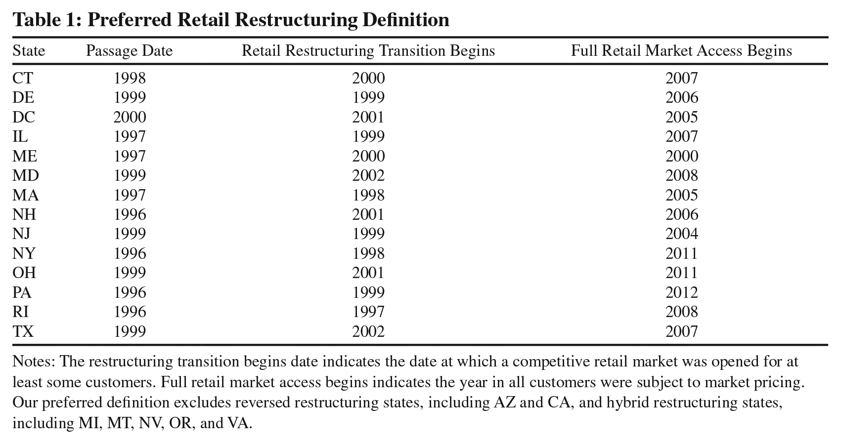
Notes: The restructuring transition begins date indicates the date at which a competitive retail market was opened for at least some customers. Full retail market access begins indicates the year in all customers were subject to market pricing. Our preferred definition excludes reversed restructuring states, including AZ and CA, and hybrid restructuring states, including MI, MT, NV, OR, and VA.

We will consider each state’s path to restructuring by two key phases. The first phase is the beginning of the restructuring transition. This phase starts with the opening of a retail market for competitive electricity suppliers to make offers to retail customers. We define this phase as a transition because it was often characterized by across-the-board discounts—usually based on the existing regulated price—and a rate freeze for customers transitioning to market prices. The second phase is when the restructuring transition ends. This phase is characterized by customers paying prices based on market prices. Several recent multi-state longitudinal studies such as Su (2015) and Ros (2017) have used EIA’s Status of Electricity Restructuring reports to determine the year of restructuring. But this report is based on the passage of legislation, rather than when the legislation was implemented. To see why this is problematic, Dormandy et al. (2019) for instance, highlight that Ros (2017) codes Ohio restructuring beginning in 2001, with the panel ending in 2009. But Ohio’s tariff mechanism that permitted customer switching coincided with the passage of Senate Bill 221 in 2008. Ours is the first analysis to specifically research each state to identify both the passage date of initial retail restructuring, but also the time it took for restructuring to be fully implemented.

We exclude seven states from our baseline analysis that have either reversed retail restructuring or have “hybrid” approaches to restructuring. We define reversed restructuring states as those that passed and subsequently repealed restructuring legislation—Arizona and California. We define hybrid states as those that did not extend full retail market competition to all customer groups—applicable to Michigan, Montana, Nevada, Oregon, and Virginia. Because reversed and hybrid states are excluded from both the treatment and control groups in our baseline analysis, our sample includes 42 territories. ²⁵ We will conduct additional robustness checks that consider hybrid and reverse states.

3. Empirical strategy

3.1 Event study

We begin with an event-study style equation:

$$P_{st}=\alpha {\sum }_{\tau =7}^{17}{\sigma }_{\tau }{Rest}_{\tau ,st}+{\gamma }_s+{\gamma }_t+{\epsilon }_{st}$$

(1)

where P_st is the average electricity price in state s, in year t. Electricity prices are presented by service class and will include residential, commercial, and industrial average electricity prices. Average electricity prices are defined as the total revenues received from these customer classes divided by the electricity used (kWh). ${\gamma }_s$ and ${\gamma }_t$ are state and year fixed effects that nonparametrically control for national trends in outcomes of interest. The variables $Res{t}_{\tau ,st}$ is an indicator variable for whether the state had passed retail restructuring reforms by that year. ${\sigma }_{\tau }$ ’s are separate indicators for each year $\mathrm{\tau }$ relative to the beginning of restructuring where $\mathrm{\tau }=0$ in the year that restructuring legislation is passed. They range from –7 to 17, taking into account the earliest and latest adopters (i.e. 1997 and 2002) alongside the sample time frame (i.e. 1990 to 2019). Restricting the treatment period in this way eliminates the potential role played by the differences in composition of states identifying various ${\sigma }_{\tau }$ ’s. For states that never implemented restructuring, all $Res{t}_{\tau ,st}$ are set equal to zero. As non-adopters, they do not play a role in the estimation of ${\sigma }_{\tau }$ but they aid in the estimation of year fixed effects, ${\gamma }_t$ as well as the constant, $\mathrm{\alpha }$ . The event study will be implemented using both the non-adopting states as well as the synthetic states made up of non-adopting states with similar ex ante characteristics, that will be discussed further below. ²⁶

We will present event-study figures that plot the estimated ${\sigma }_t$ ’s against $\tau$ . These figures provide an opportunity to visually assess trends in the outcome variables prior to retail restructuring passage, which aids in assessing the validity of the remainder of differences-in-differences results. The event-study figures also demonstrate the timing of the effect. Of particular interest in this context, implementation of full retail market access took years in many instances. Thus, perhaps effects immediately after passage, i.e. during the transition period, are different than longer term effects.

3.2 Difference-in-Differences

Equation (2) illustrates the difference-in-differences estimation strategy that will be utilized for the remainder of empirical tests.

$$P_{st}=\alpha +\delta Res{t}_{st}+{\gamma }_s+{\gamma }_t+{\epsilon }_{st}$$

(2)

Where again $P_{st}$ is the average electricity price in state, s, in year t. $Res{t}_{st}$ is an indicator variable for the time periods after retail restructuring was implemented in each treated state. The treated states and the corresponding years of treatment for each state are presented in Table 1. State-level fixed effects, ${\gamma }_s$ , and time fixed effects, ${\gamma }_t$ , are included in all regressions, absorbing the effect of the restructured state and post-restructuring indicator variables. Standard errors are clustered at the state level as recommended by Bertrand et al. (2004). The time period of the analysis is from 1990 to 2019.

As shown in Table 1, there were significant lags in when the restructuring process began and full retail-restructuring implementation occurred. To account for this, we modify equation (2) to separate test for the effect during the transition period and post-full implementation:

$$P_{st}=\alpha +{\delta }_{1}Transitio{n}_{st}+{\delta }_{2}FullIm{p}_{st}+{\gamma }_s+{\gamma }_t+{\epsilon }_{st}$$

(3)

Where $Transitio{n}_{st}$ is one during the transition period and zero before and after post-full retail-restructuring implementation and $FullIm{p}_{st}$ is one post full retail-restructuring implementation and zero in all years pre-full implementation. $\delta$ and ${\delta }_2$ are the coefficients of interest and represent the treatment effect during the transition and full implementation.

We present two sets of empirical estimates which utilize this difference in differences framework. First, as a baseline, we use the 14 territories (13 states plus Washington DC) that did restructure as the treatment group compared to the 28 states that did not restructure as the control group. The estimated δ provides the change in total, residential, commercial, and industrial electricity prices in restructured states relative to non-restructured states after policy adoption—but does not address endogenous adoption of policies. We purposely do not include any control variables in this baseline specification to provide a descriptive analysis of what occurred in restructured states relative to COS states after implementation. A comparison of state-level point estimates to the synthetic control estimates discussed below provide insight into the importance of addressing the endogeneity of implementing restructuring.

Next, we will test for potential impacts on relative rates between customer groups. We empirically examine the potential for cross subsidization between customer classes by modifying Equation (2), including the log price-differential between residential and commercial and industrial customers as the dependent variable in our difference-in-differences model.

Importantly, we will consider three treatment time definitions discussed in Section 2.1. Specifically, we will consider all post treatment which includes the beginning of retail restructuring through the end of the sample. We will then estimate separately the effect of the transition period and post full retail market access.

3.3 Choosing a Control Group

Given that policy adoption is not randomly assigned to states (Craig, 2016; Guerriero, 2020), we will construct a synthetic control state for each treated state that will be utilized in the empirical tests. The synthetic controls are created by taking a weighted average of non-treated units, so in this application each synthetic state will be constructed as a weighted average of the 28 states that have similar pre-treatment characteristics to the treated states, but that did not undergo any restructuring. ²⁷ The idea behind this approach is that a combination of states might provide a better comparison to the treated states post restructuring than any single state (Abadie, Diamond, & Hainmueller, 2010). State level restructuring policies is an ideal application of synthetic control methods because we are interested in estimating the treatment effect of a policy intervention on aggregated units (i.e. U.S. states).

Economic characteristics used to construct synthetic controls (SCs) include total gross state product (GSP) per person, GSP per person associated with manufacturing and GSP per person associated with mining. Political characteristics include the percent of the state legislature that is affiliated with the Democratic Party as well as an indicator variable for whether the governor of the state is a Democrat. We consider the total share of the total electricity consumption in the state associated with commercial and industrial customers (with the residual share approximately being residential electricity demand) as well as the share of generating capacity by state from natural gas, the marginal fuel source. Importantly, synthetic controls are created ex ante to policy passage, and so any endogenous impact of retail restructuring on any of these factors used to construct SCs will not impact empirical results.

The difference in outcomes (prices) in the synthetic states compared to the restructured states will provide an estimated treatment effect. We will pool all restructured states and synthetic states into one regression and estimate the treatment effect using the difference-in-differences framework shown in Equation (2). This will provide the average treatment effect of retail restructured compared to synthetic non-restructured states for each outcome of interest—electricity prices for each customer class. Average electricity prices in treated states relative to their synthetic controls are presented in Appendix Figure A1. Robustness checks will show restructured states relative to synthetic controls alongside randomly assigned placebo intervention on non-treated states relative to synthetic controls.

3.4 Potential Mechanisms

We explore two potential mechanisms for the result that electricity prices generally increased in restructured states post retail restructuring. First, we explore whether renewable energy generation growth was higher in retail-restructured states. Second, we explore whether retail electricity prices were more sensitive to natural gas prices due to restructuring policies. ²⁸

3.4.1 Renewable Energy Generation

Retail choice can enable customers to choose to purchase renewable energy, typically for a small premium on their electricity bill. The customer’s choice to procure renewable energy will ensure that system wide, that amount of renewable energy will be produced and therefore used. Thus, it is possible that retail restructuring has both increased electricity price and renewable energy generation through this channel.

While not specifically focusing on restructuring policies, in the academic literature, renewable energy policies have been associated with higher electricity prices (Upton & Snyder, 2017; Young & Bistline, 2018; Greenstone & Nath 2020). If retail restructuring has impacted renewable energy generation, this could be one channel through which retail rates can be impacted. In fact, all restructured states also implemented renewable portfolio standards (RPSs) and many restructured states are part of the Regional Greenhouse Gas Initiative (RGGI). ²⁹

As a robustness check, we re-run our baseline specification testing the effect of retail restructuring on renewable energy generation per person, as this is one mechanism through which restructuring might have impacted retail rates. Point estimates suggest that that renewable energy generation decreased in fully restructured states, albeit results are statistically marginal. This suggests it is unlikely that renewable energy growth is driving the observed electricity price increases in restructured states.

3.4.2 Natural Gas Price Sensitivity

Prior analysis has shown that electricity prices generally increased in the post-retail restructuring era. But retail restructuring happened to generally coincide with an increase in natural gas prices nationally. The evidence from Figure A2 suggests that the restructured states experienced higher sensitivity to natural gas prices. Further, comparing the event studies in Figure 1, the difference in electricity prices in restructured and non-restructured states is not statistically different in the latter years of the sample; i.e. from about 12 years post-restructuring to the end of the sample. Together, these figures suggest that retail electricity prices were more responsive to natural gas prices due to retail restructuring.

All prior analyses control for natural gas prices, to the extent that prices vary consistently across time and states, through the inclusion of state and year fixed effects. But the price that electric power producers pay can vary across both time and states due to factors unrelated to restructuring policies. For instance, pipeline constraints and relief of those constraints have been shown to create spatial and temporal deviation of hydrocarbon prices from benchmark prices for both oil and natural gas (Plante & Strickler, 2019; Agerton & Upton, 2019; Walls & Zheng 2020; Agerton, Gilbert & Upton, 2020).

Ideally, a yearly panel of natural gas prices paid by electric power producers by state would be available over the sample time period of this analysis, i.e. 1990 to 2019. Unfortunately, this is not available. The closest data set that is available includes natural gas electric power prices across states and years, but this data is imperfect for two reasons. ³⁰ First, the data is only available from 1997. The earliest state, Rhode Island, had already begun restructuring at the that time, and therefore no pre-treatment data would be available. All states that would implement restructuring had begun the process of transitioning by 2002, as shown in Table 1.

Second, this dataset has missing information. For example, Texas data is complete, showing yearly observations from 1997 to 2019. But Connecticut, another restructured, state has missing data for the years 2000, 2003, and 2004. On the other end of the spectrum, Delaware data is not available after 2002.

While imperfect, we will utilize this data to test whether electricity retail prices became more sensitive to changes in natural gas prices due to restructuring. To do so, we first regress natural gas price sold to electric power producers on state and year fixed effects.

$$NG{P}_{st}={\gamma }_s+{\gamma }_t+{\epsilon }_{st}$$

(4)

We then obtain ${\widehat{NGP}}_{st}$ and replace all missing values of $NG{P}_{st}$ with ${\widehat{NGP}}_{st}$ . In doing so, we create a balanced panel of 50 territories over 23 years, totaling 1,150 observations. Of these, 379 values are predicted, making up about one third of the sample. We then modify equation (2) and (3) to include restructuring interacted with natural gas prices as shown in (5) and (6):

$$P_{st}=\alpha +\eta Res{t}_{st}+\delta \left(Res{t}_{st}\times NG{P}_{st}\right)+\varphi \left(\left(1-Res{t}_{st}\right)\times NG{P}_{st}\right){X^{\prime }}_{st}\mathrm{\beta }+{\gamma }_s+{\gamma }_t+{\epsilon }_{st}$$

(5)

$$\begin{array}{c}{P}_{st}=\alpha +{\eta }_{1}Transitio{n}_{st}+{\eta }_{2}FullIm{p}_{st}+{\delta }_1(Transitio{n}_{st}\times NG{P}_{st})+{\delta }_2(FullIm{p}_{st}\times NG{P}_{st})\\ +\varphi \left(\left(1-Res{t}_{st}\right)\times NG{P}_{st}\right)+{X^{\prime }}_{st}\mathrm{\beta }\mathrm{+}{\gamma }_s+{\gamma }_t+{\epsilon }_{st}\end{array}$$

(6)

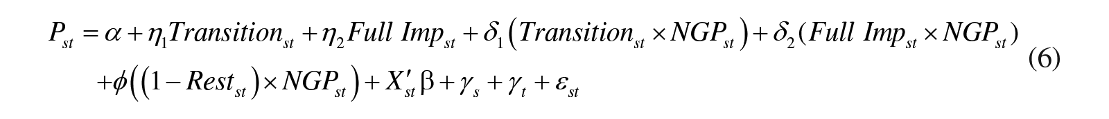
These equations interact restructuring with natural gas prices to test for whether prices in restructured states are more sensitive to natural gas price changes post restructuring. We include control variables, $X_{st}$ , including the share of electricity generating capacity from natural gas, the renewable energy generation (in kWh per person), and the cooling degree days (CDDs). ³¹ Because approximately one third of the data from $NG{P}_{st}$ is predicted values from equation (4), standard errors are bootstrapped. If retail restructuring policies increased the sensitivity of retail electricity prices to natural gas prices paid by electric power producers, we anticipate for $\mathrm{\delta }>\mathrm{\phi }$ .

3.5 Robustness Checks

We next conduct robustness checks.

3.5.1 Hybrid/Reversal States

In our baseline specification, we removed seven states that either implemented what we consider a “hybrid policy” or decided to reverse a retail restructuring policy. We argue that removing these states is important to clearly identify treated and non-treated units which serve as the foundation of our analysis. But, as an additional robustness check, we examine the impact of retail restructuring on these hybrid/reverse states relative to both non-restructured states and SCs. We will implement an event study using both control groups and by customer class for hybrid/reversal states.

3.5.2 Placebo Treatment

Similar to Abadie, Diamond & Hainmueller (2010), Abadie and Gardeazabal (2003) and Bertrand Duflo, and Mullainathan (2004), we next implement placebo studies by applying the synthetic control method to states that did not implement retail electricity market restructuring. Specifically, we employ two placebo tests. First, motivated by Bertrand Duflo, and Mullainathan (2004), we randomly assign treatment to states across the years of actual treatment for the policies (i.e. 1998 to 2002). Next, we construct synthetic states for the 28 non-restructured states as a weighted average of other untreated states. We estimate a pooled treatment effect using Equation (2) and expect that these treatment effects will be randomly distributed around zero.

3.5.3 Bias from Staggered Treatment Adoption

Recently methodological critiques of the two-way fixed effects difference-in-differences approaches with variation in treatment timing have become prevalent in the literature, imploring additional robustness checks. Goodman-Bacon (2018) has shown that with staggered treatment adoption—applicable in our analysis as states restructured at different points in time—standard two-way fixed effects estimators produce a variance-weighted average of all possible difference-in-differences estimates. With treatment effect heterogeneity, either across states or over time, estimates can be biased as early treated states may serve as an effective control state for later treated states. Sun and Abraham (2021) have shown that results can even be of the opposite sign if early treated states’ restructuring outcomes changed over time.

To address this potential bias, we employ a stacked regression similar to Cengiz et al. (2019), where we align event study datasets for when each state implements restructuring in relative time to eliminate the possibility that early treated states are utilized as controls for later treated states. For each state that undergoes restructuring in a particular year we define a group, g, and create a unique dataset that consists of that group of states that restructured in each year, and control states from states that never restructured. We assign a 24-year estimation window (t= –7 to t=17), stack datasets in relative time, and estimate and average treatment effect of retail restructuring across all restructured states. Our estimating equation is:

$$P_{gt}={\alpha }_g+{\sum }_{k=7}^7{\sigma }_{k}I\left[t-Res{t}_{st}=k\right]+{\gamma }_g+{\gamma }_{tg}+{\epsilon }_{gt}$$

(7)

where $P_{gt}$ is the average electricity price in the group of states g, implementing restructuring in year t. ${\gamma }_g$ and ${\gamma }_{gt}$ are group and year fixed effects. The variable $Res{t}_{st}$ is an indicator variable for whether a state passed restructuring reforms in year t, and $I\left[t-Res{t}_{st}=k\right]$ indicates a state is k years away from restructuring.

3.5.4 Falsification Outcomes

Next, we implement two falsification tests. We estimate a treatment effect on two outcomes that we do not expect to be impacted by retail electricity market restructuring. First, we estimate a treatment effect on state level cooling degree days (CDDs). While CDDs are commonly used to predict electricity demand, CDDs are a function of the weather and therefore state level policies should have no impact on future weather (in that state). If we find that policy adoption leads to changes in the weather, we will have reason to be concerned.

While the SC approach can account for observable factors that impact non-random policy adoption, this approach is imperfect in that it does not control for unobservable factors that can simultaneously impact the choice to restructure and outcomes of interest, potentially biasing results. For this reason, we implement a second falsification test to address the extent to which unobservable factors are plausibly driving results of the SC analysis. Specifically, the second falsification test outcome is state-wide demand for motor gasoline. This is chosen because it is an alternative form of energy demand that should not be impacted by retail electricity market restructuring but might be impacted by unobserved shocks that would simultaneously impact policy adoption and the outcomes of interest.

4. Results

4.1 Summary Statistics

Summary statistics for the treatment and control groups pre- and post-2002 are shown in Table 2. We choose the date 2002 (for discussion purposes only) as this was the latest date for which a state began the restructuring process. We show averages for electricity prices by customer class (the four outcome variables of interest) and the three other outcome variables used in various mechanism and robustness specifications (renewable energy generation, CDDs, and gasoline demand).

Table 2

Summary Statistics

	Treatment Group			Control Group
State-Level Electricity Prices	Pre 2002	Post 2002	Percent Change	Pre 2002	Post 2002	Percent Change	% Change Treatment –% Change Control
Total (cents/kWh)	8.52	11.90	40%	5.80	8.08	39%	0.4%
Residential (cents/kWh)	10.18	13.85	36%	7.11	9.86	39%	–2.6%
Commercial (cents/kWh)	8.77	11.56	32%	6.28	8.38	33%	–1.6%
Industrial (cents/kWh)	6.27	8.91	42%	4.23	5.87	39%	3.3%
Additional Outcome Variables Renewable Energy Generation Per Person (kWh/year)	1,738	1,976	14%	4,100	5,365	31%	–17.2%
Cooling Degree Days	776	900	16%	1,121	1,228	10%	6.4%
Gasoline Consumption Per Person (gallons/person/day)	1.21	1.12	–7%	1.38	1.32	–4%	–3.1%

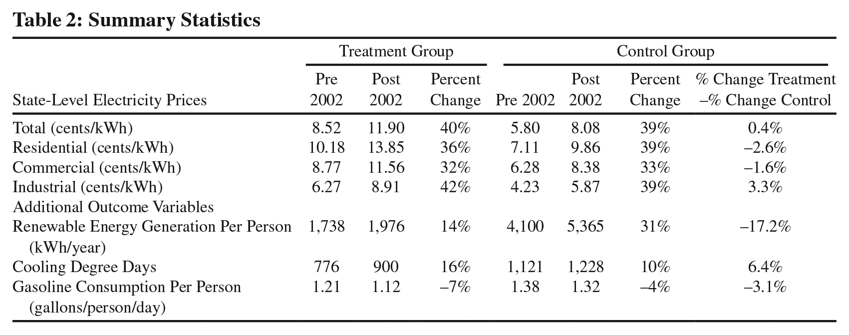
A simple look at the average percent change in prices in the two groups pre- and post-2002 in Table 2 reveals relatively little change in average prices in the two groups. Average prices increased by 3.38 cents per kWh, or about 40 percent, in the treatment group, and 2.28 cents per kWh, or 39 percent in the control group. What is also noticeable is that states that would later restructure had higher prices in the pre-restructuring era. Thus, a simple examination of these summary statistics does not show evidence that retail restructuring policies were effective at reducing electricity prices.

Restructured states have less renewable energy generation per-capita both pre- and post-restructuring, and renewable generation per person grew at a faster rate in the non-restructured states. Restructured states also experienced faster declines in gasoline consumption per capita than non-restructured states.

Appendix Table A2 shows summary statistics for the treatment group, control group, and hybrid/reversal states separately. Table A2 also shows summary statistics for the variables used to construct synthetic controls namely: GSP per person, mining GSP per person, manufacturing GSP per person, the party of the governor, the percent of the legislature that are Democrats, the share of generating capacity from natural gas, the share of electricity sales to industrial customer, and the share of sales to commercial customers. Focusing on variables used to construct SCs, treated states had higher GSP per person than non-treated states. Treated states were also less mining intensive than control states and had similar manufacturing GSP per person. Restructured states were also less likely to have a democratic governor in the pre-restructuring era, but slightly more likely to have a democratic legislature. Restructured states also had a higher share of generating capacity from natural gas than non-restructured states.

4.2 Synthetic Control (SC) Trends

Appendix Figure A2 graphically presents the synthetic control analysis, which compares average electricity rates in restructured (treated) units relative to non-restructured (control) units and synthetic control units with similar economic and political characteristics. Trends are shown for average rates and by customer class; residential, commercial, and industrial. Also shown in Figure A2 is the number of states that passed restructuring laws and the number of states for which retail market access began over the sample period; these corresponding dates are listed in Table 1. Because we remove all reverse and hybrid states from analysis, all fourteen states that pass restructuring laws also eventually gain retail market access. Thus, by design the latter moves with a lag to the former.

Upon visual inspection, the first observation is that synthetic states and naïve non-restructured states have very similar trends in both the pre- and post-restructuring time period. This will be confirmed with event study results presented below.

The second observation is that restructured states tended to experience an increase in electricity rates relative to both the non-restructured states and synthetic controls (SCs) from 2005 to about 2009. Then, around 2010, the prices in restructured states began to converge with non-restructured SCs. There is less evidence of this convergence for residential customers; this trend break is most obviously observed for industrial customers.

Appendix Figure A3 compares the difference in treated and SC states with natural gas prices. The difference in the price per kWh in restructured states and synthetic control states (from Appendix Figure A2) is shown on the left vertical axis. From 1990 until the early 2000s, the difference in prices between the two groups ranged from 2 to 3 cents per kWh, with states that would eventually restructure having higher prices than the SC states. But when the price of natural gas began to rise in the mid to late 2000s, the price of electricity in restructured states increased. When natural gas prices dropped in 2009, the difference in electricity prices between restructured and non-restructured states began to collapse. This is graphical evidence that retail customer prices more closely followed wholesale prices in restructured states. Figure A3 further shows these trends for residential, commercial, and industrial customer classes.

4.3 Event Study

Figure 1 presents event study results. ³² These event studies corroborate the broad observations from Figures A2 and A3. Importantly, there is no statistically significant pre-trend difference in prices in treated and control states in the pre-restructuring era and the event studies look very similar using both the baseline and synthetic control groups. In fact, it is difficult to see any difference in the two event studies.

Event studies also reveal information about the potential timing of restructuring on prices. Specifically, analyzing both control groups, event studies show that electricity prices did experience small but statistically insignificant reductions in retail prices for about two years after the policies were passed. But beginning two years after passage until eight years post-passage, restructured states experienced yearly increases in prices relative to controls. But then, the trend began to reverse itself, and by approximately twelve years post-restructuring, prices in the treatment and control groups were no longer statistically significantly different, and they have exhibited approximately a parallel trend since. Thus, the event study reveals that restructuring states did experience increases in prices in the post-restructuring years, but these prices have since re-converged.

These event studies motivate the potential importance of considering the phases of restructuring and motivate a test for the mechanism for this price increase, namely increased sensitivity to natural gas prices, that will be presented in subsequent analyses.

Figure 1

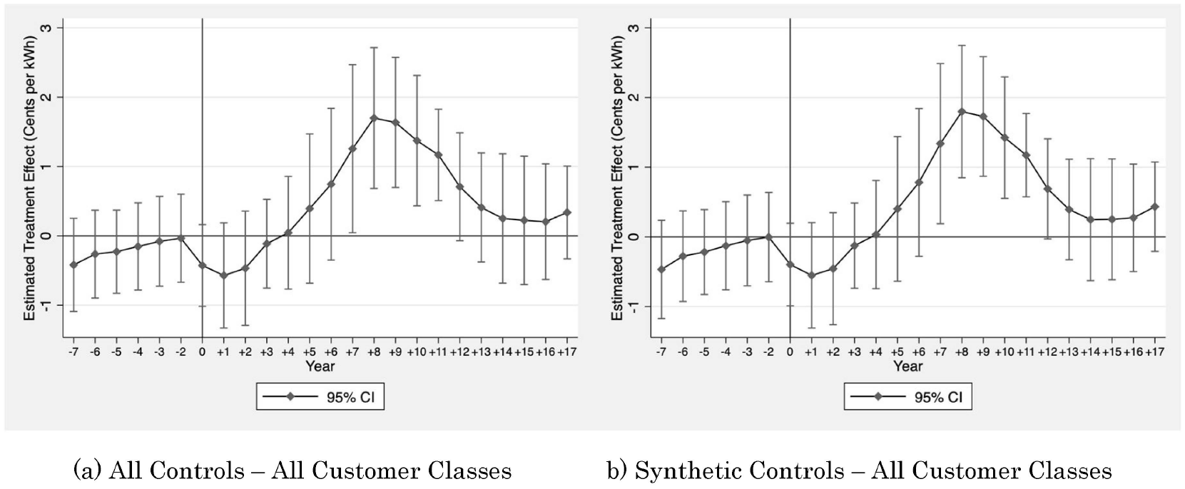
Event Study—Effect of Retail Restructuring on Retail Electricity Prices

4.4 Difference-in-Differences (DD) Results

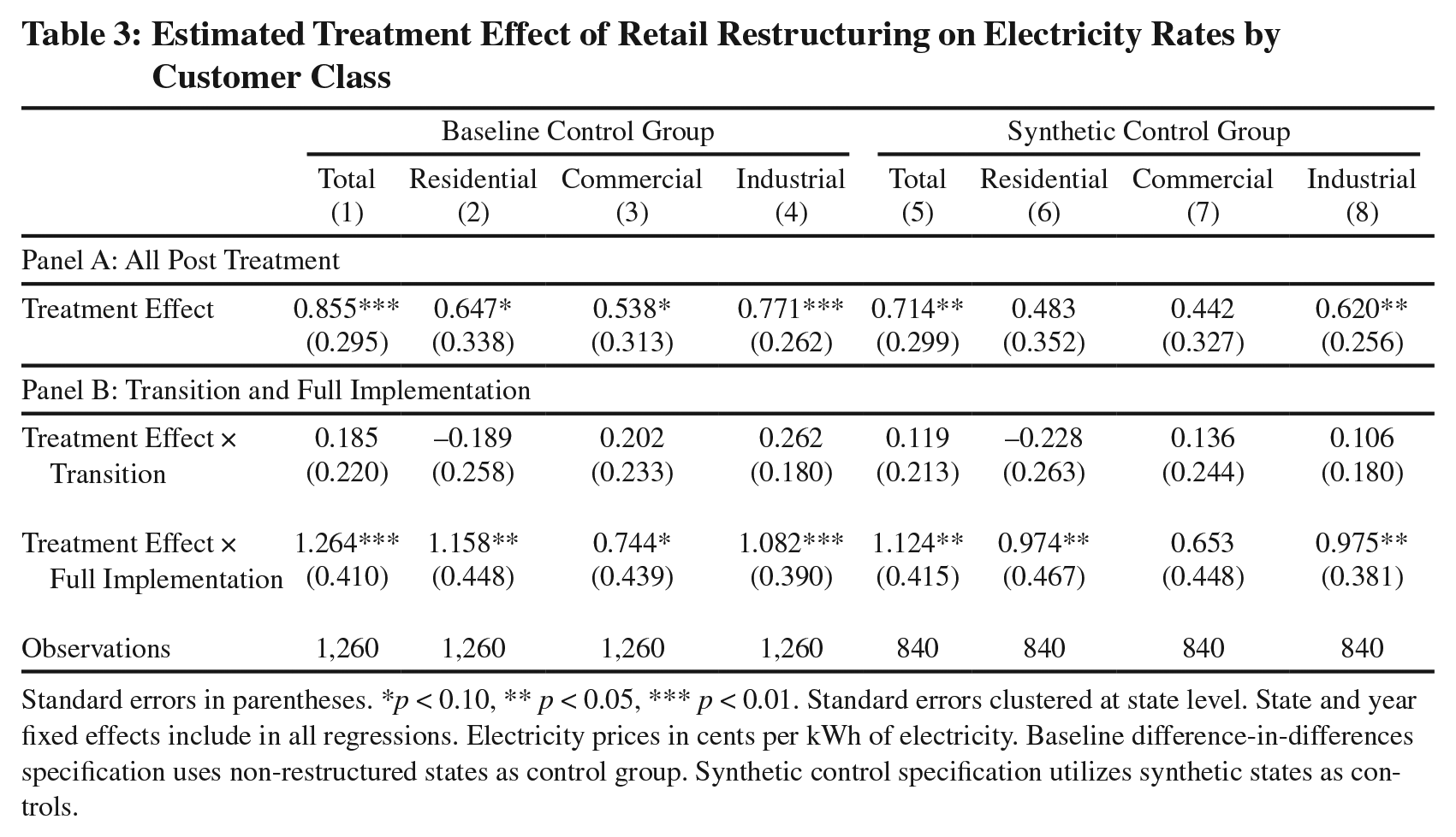
Main regression results are presented in Table 3. We present results for three definitions of treatment effects. In Panel A we consider all years post-retail restructuring transition beginning as defined in Table 1 (see equation (2)). In Panel B, we separately consider the transition and full implementation, also shown in Table 1 (equation (3)).

Table 3

Estimated Treatment Effect of Retail Restructuring on Electricity Rates by Customer Class

	Baseline Control Group				Synthetic Control Group
	Total	Re sidential	Commercial	Industrial	Total	Residential	Commercial	Industrial
	(1)	(2)	(3)	(4)	(5)	(6)	(7)	(8)
Panel A: All Post Treatment
Treatment Effect	0.855***	0.647*	0.538*	0.771***	0.714**	0.483	0.442	0.620**
	(0.295)	(0.338)	(0.313)	(0.262)	(0.299)	(0.352)	(0.327)	(0.256)
Panel B: Transition and Full Implementation
Treatment Effect × Transition	0.185	–0.189	0.202	0.262	0.119	–0.228	0.136	0.106
	(0.220)	(0.258)	(0.233)	(0.180)	(0.213)	(0.263)	(0.244)	(0.180)
Treatment Effect × Full Implementation	1.264***	1.158**	0.744*	1.082***	1.124**	0.974**	0.653	0.975**
	(0.410)	(0.448)	(0.439)	(0.390)	(0.415)	(0.467)	(0.448)	(0.381)
Observations	1,260	1,260	1,260	1,260	840	840	840	840

Standard errors in parentheses. *p < 0.10, ** p < 0.05, *** p < 0.01. Standard errors clustered at state level. State and year fixed effects include in all regressions. Electricity prices in cents per kWh of electricity. Baseline difference-in-differences specification uses non-restructured states as control group. Synthetic control specification utilizes synthetic states as controls.

Table 3 includes eight columns of results. Columns (1)–(4) show results using the baseline control group for all customers: residential, commercial, and industrial respectively. These results provide a description of changes in prices pre- and post-retail restructuring. Columns (5)–(8) present results using the synthetic control groups. In these regressions, we use the synthetic state for each of the fourteen treated states.

Focusing on columns (1)–(4), we see that prices generally increased in restructured states post-restructuring relative to non-treated states. We find a statistically significant 0.86 cent/kWh increase associated with all post treatment time period shown in Panel A. We do not find evidence of price changes between the two groups in the transition period shown in Panel B, with treatment effects orders of magnitude smaller and statistically insignificant. Specifically, Panel B finds that prices increased by 1.3 cents per kWh in restructured states post full implementation of retail restructuring.

Next, focusing on columns (5)–(8), we make two broad observations. First, the magnitude of the point estimates is smaller compared to the baseline control group. But second, the overall conclusion and standard errors are similar. Focusing on all customer classes, we find that prices increased by about 1.2 cents per kWh in restructured states relative to SCs once full retail access was implemented: as shown in column (5) of Panel B.

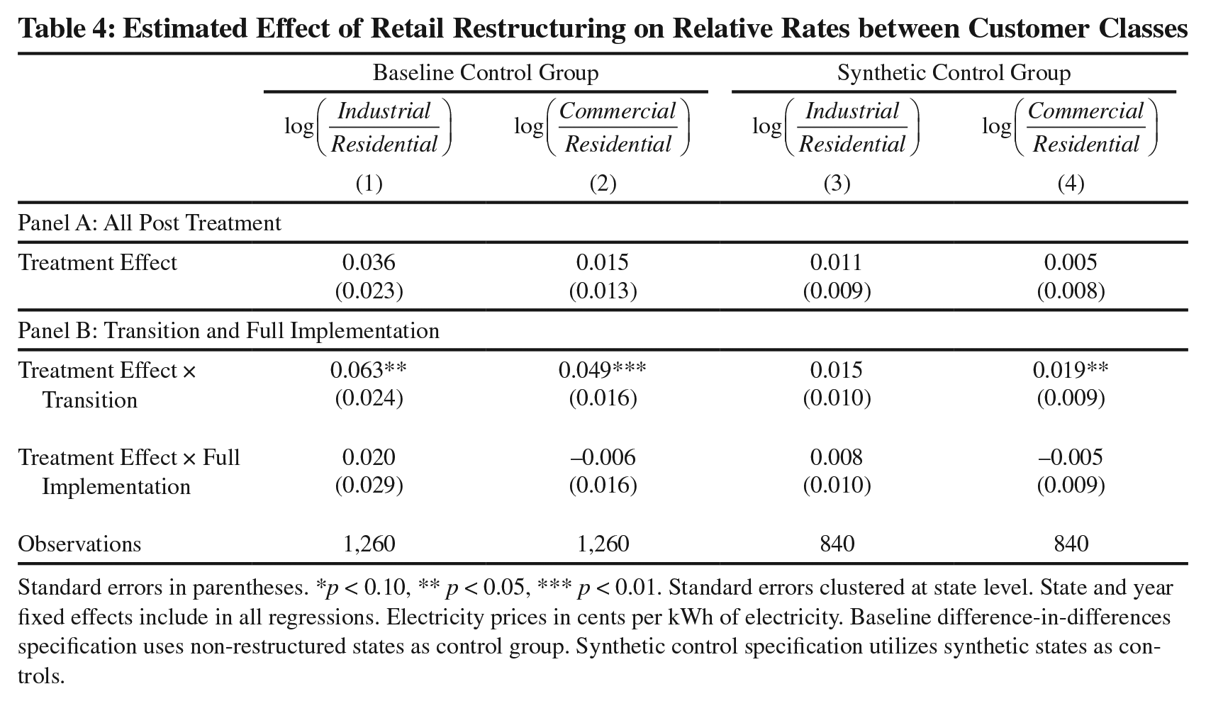
Next, Table 4 tests for the effect of retail restructuring on the relative change in prices between customer classes. We consider the ratio of commercial and industrial to residential prices. Focusing on the SC results in Columns (3) and (4), we find evidence that commercial rates increased relative to residential rates during the transition period, but these do not persist into the longer term once full retail access begins. Thus, we do not find evidence of long-run effects of retail restructuring on electricity prices between rate classes.

Table 4

Estimated Effect of Retail Restructuring on Relative Rates between Customer Classes

Baseline Control Group		Synthetic Control Group
$\log \left(\frac{Industrial}{Residential}\right)$	$\log \left(\frac{commercial}{Residential}\right)$	$\log \left(\frac{Industrial}{Residential}\right)$	$\log \left(\frac{commercial}{Residential}\right)$
(1)	(2)	(3)	(4)
Panel A: All Post Treatment
Treatment Effect	0.036	0.015	0.011	0.005
	(0.023)	(0.013)	(0.009)	(0.008)
Panel B: Transition and Full Implementation
Treatment Effect × Transition	0.063**	0.049***	0.015	0.019**
	(0.024)	(0.016)	(0.010)	(0.009)
Treatment Effect × Full Implementation	0.020	–0.006	0.008	–0.005
	(0.029)	(0.016)	(0.010)	(0.009)
Observations	1,260	1,260	840	840

Standard errors in parentheses. *p < 0.10, ** p < 0.05, *** p < 0.01. Standard errors clustered at state level. State and year fixed effects include in all regressions. Electricity prices in cents per kWh of electricity. Baseline difference-in-differences specification uses non-restructured states as control group. Synthetic control specification utilizes synthetic states as controls.

4.5 Potential Mechanisms

4.5.1 Renewable Energy Generation

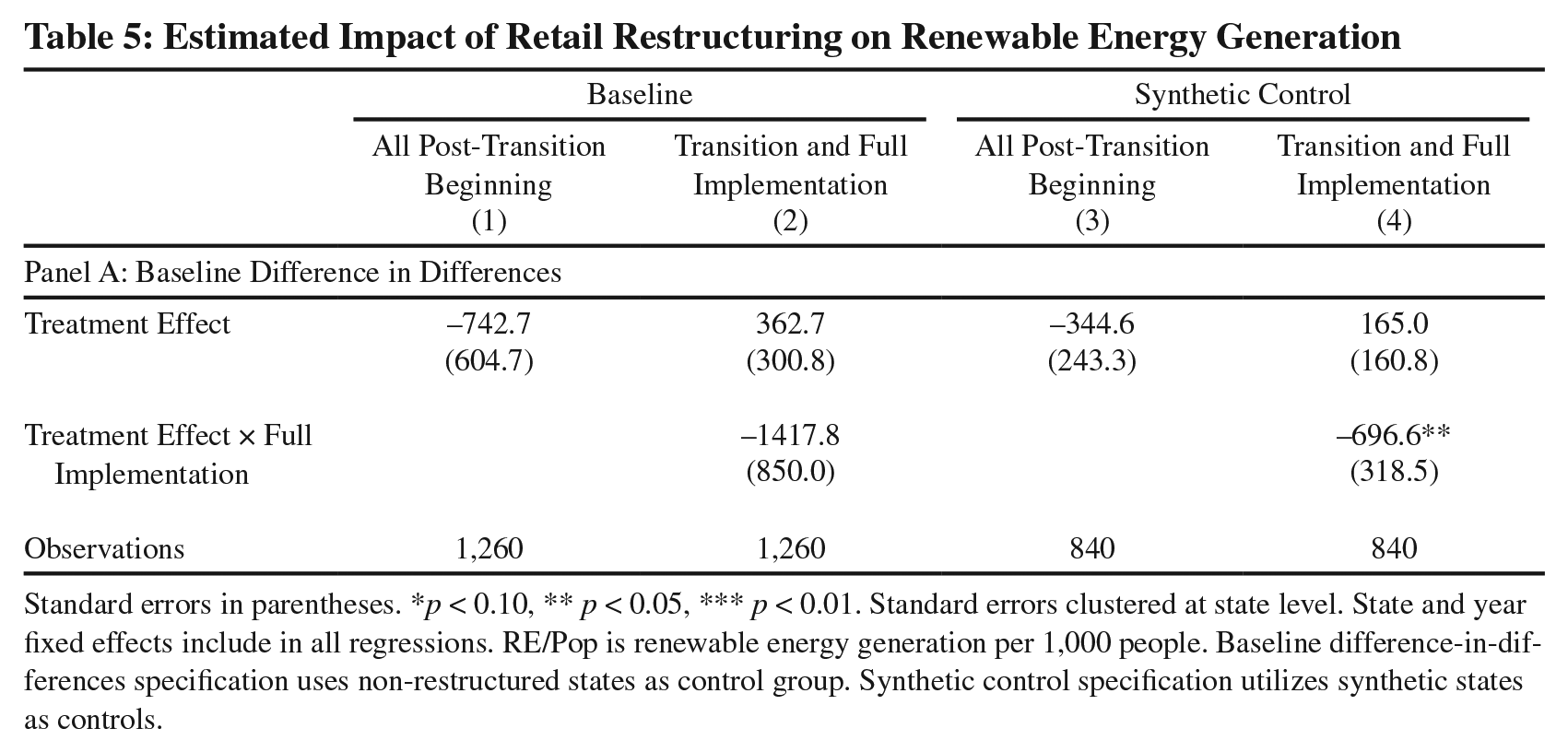
We next consider the extent to which retail restructuring policies might have facilitated renewable energy generation growth. ³³ To do so, we simply implement our DD estimation strategy utilizing renewable energy generation per person as an outcome variable. Results are presented in Table 5.

Table 5

Estimated Impact of Retail Restructuring on Renewable Energy Generation

	Baseline		Synthetic Control
	All Post-Transition Beginning	Transition and Full Implementation	All Post-Transition Beginning	Transition and Full Implementation
	(1)	(2)	(3)	(4)
Panel A: Baseline Difference in Differences
Treatment Effect	–742.7	362.7	–344.6	165.0
	(604.7)	(300.8)	(243.3)	(160.8)
Treatment Effect × Full Implementation		–1417.8		–696.6**
		(850.0)		(318.5)
Observations	1,260	1,260	840	840

Standard errors in parentheses. *p < 0.10, ** p < 0.05, *** p < 0.01. Standard errors clustered at state level. State and year fixed effects include in all regressions. RE/Pop is renewable energy generation per 1,000 people. Baseline difference-in-differences specification uses non-restructured states as control group. Synthetic control specification utilizes synthetic states as controls.

Focusing on the SC specification, we find that renewable energy generation decreased by about 696.6 kWh per year once retail restructuring was fully implemented. For perspective, the average state produced about 6,948 kWh per person in the most recent year of data, 2019. We do not interpret this that retail restructuring had a negative causal effect on renewable electricity generation, per se, as we leave this question for future research. But this result does suggest that increased renewable penetration is not a plausible mechanism driving electricity price increases observed in restructured states.

4.5.2 Sensitivity to Natural Gas Prices

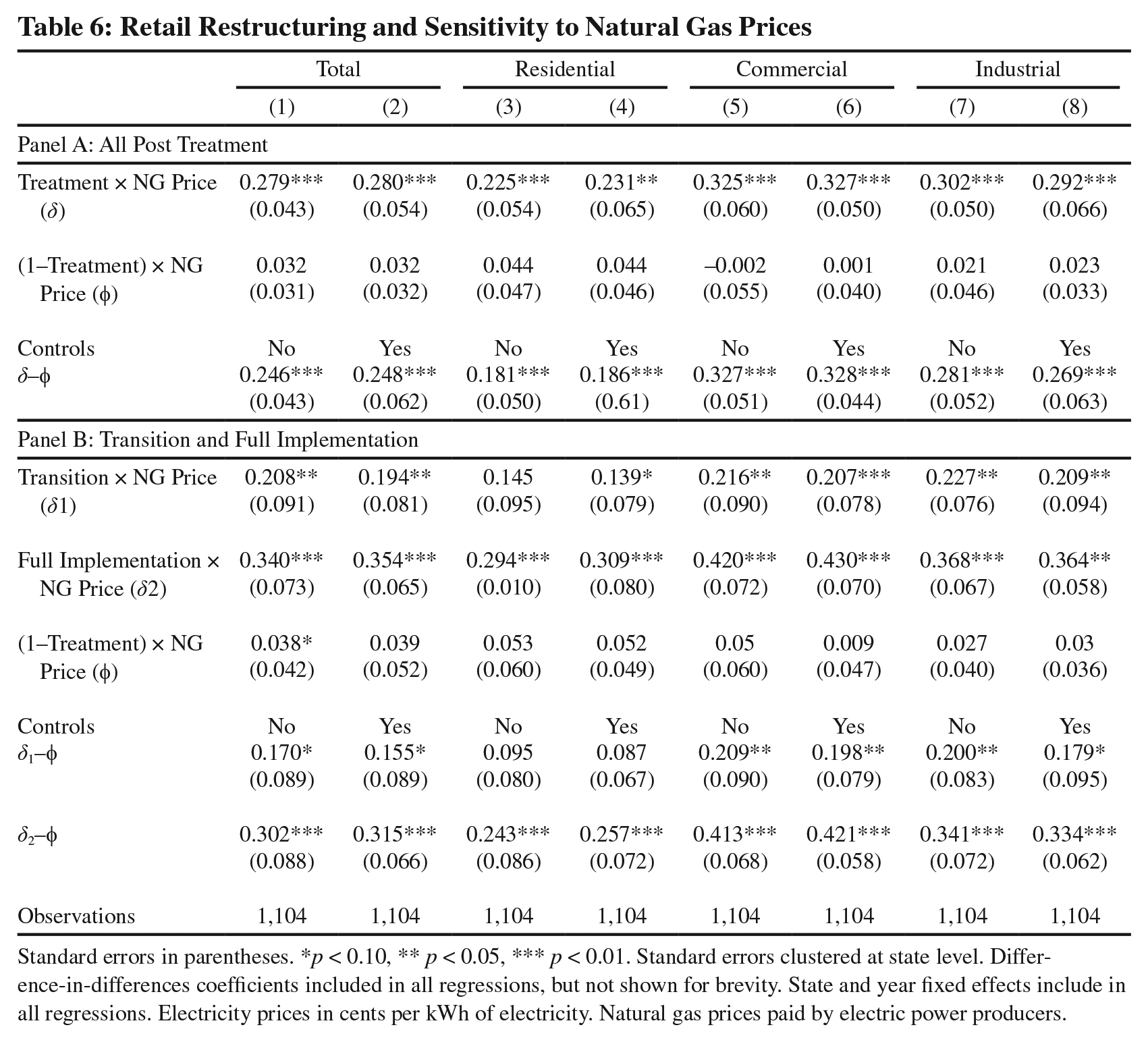
We next explore whether electricity prices responded more to natural gas price changes due to retail restructuring. We present results for all four customer classes and with and without controls utilizing the empirical specifications presented in equations (5) and (6). Results are presented in Table 6. We note a few observations, focusing on Panel B which shows results of both the transition period and full implementation.

Table 6

Retail Restructuring and Sensitivity to Natural Gas Prices

	Total		Residential		Commercial		Industrial
	(1)	(2)	(3)	(4)	(5)	(6)	(7)	(8)
Panel A: All Post Treatment
Treatment × NG Price (δ)	0.279***	0.280***	0.225***	0.231**	0.325***	0.327***	0.302***	0.292***
	(0.043)	(0.054)	(0.054)	(0.065)	(0.060)	(0.050)	(0.050)	(0.066)
(1–Treatment) × NG Price (φ)	0.032	0.032	0.044	0.044	–0.002	0.001	0.021	0.023
	(0.031)	(0.032)	(0.047)	(0.046)	(0.055)	(0.040)	(0.046)	(0.033)
Controls	No	Yes	No	Yes	No	Yes	No	Yes
δ–φ	0.246***	0.248***	0.181***	0.186***	0.327***	0.328***	0.281***	0.269***
	(0.043)	(0.062)	(0.050)	(0.61)	(0.051)	(0.044)	(0.052)	(0.063)
Panel B: Transition and Full Implementation
Transition × NG Price (δ1)	0.208**	0.194**	0.145	0.139*	0.216**	0.207***	0.227**	0.209**
	(0.091)	(0.081)	(0.095)	(0.079)	(0.090)	(0.078)	(0.076)	(0.094)
Full Implementation × NG Price (δ2)	0.340***	0.354***	0.294***	0.309***	0.420***	0.430***	0.368***	0.364**
	(0.073)	(0.065)	(0.010)	(0.080)	(0.072)	(0.070)	(0.067)	(0.058)
(1–Treatment) × NG Price (φ)	0.038*	0.039	0.053	0.052	0.05	0.009	0.027	0.03
	(0.042)	(0.052)	(0.060)	(0.049)	(0.060)	(0.047)	(0.040)	(0.036)
Controls	No	Yes	No	Yes	No	Yes	No	Yes
δ1–φ	0.170*	0.155*	0.095	0.087	0.209**	0.198**	0.200**	0.179*
	(0.089)	(0.089)	(0.080)	(0.067)	(0.090)	(0.079)	(0.083)	(0.095)
δ2–φ	0.302***	0.315***	0.243***	0.257***	0.413***	0.421***	0.341***	0.334***
	(0.088)	(0.066)	(0.086)	(0.072)	(0.068)	(0.058)	(0.072)	(0.062)
Observations	1,104	1,104	1,104	1,104	1,104	1,104	1,104	1,104

Standard errors in parentheses. *p < 0.10, ** p < 0.05, *** p < 0.01. Standard errors clustered at state level. Difference-in-differences coefficients included in all regressions, but not shown for brevity. State and year fixed effects include in all regressions. Electricity prices in cents per kWh of electricity. Natural gas prices paid by electric power producers.

First, we find generally insignificant effect of natural gas prices on retail prices in the non-restructured states/time periods. Of the eight coefficients estimated, one is statistically significant at the ten percent level. Point estimates, though, are consistently positive. For example, when controls are included, we estimate that a $1 change in natural gas prices per thousand cubic feet (mcf) is associated with a 0.039 cent per kWh increase in the electricity price.

Second, during the transition period, we find a statistically significant relationship between natural gas prices for all customer classes. Natural gas prices have the smallest effect on residential prices during the transition period, with results also marginally statistically significant. In all eight regressions, the magnitude of these estimates $({\delta }_1)$ is larger than the non-treatment coefficient $\left(\mathrm{\phi }\right)$ . Specifically, when controls are included, we estimate that a $1 change in natural gas prices per mcf is associated with a 0.194 cent per kWh increase in the electricity price.

Third, analyzing the full implementation time period, we observe that the magnitude of the point estimates approximately double across all regressions. Again, focusing on total electricity prices when controls are included, we estimate that a $1 change in natural gas prices per mcf is associated with a statistically significant 0.35 cent per kWh increase in the electricity price.

An empirical test for ${\delta }_2-\varphi$ is presented testing whether the sensitivity to natural gas prices increased post-full retail restructuring. Point estimates suggest that electricity prices increased by 0.315 cents per kWh for a $1 per mcf change in natural gas prices, empirically supporting the general observation that prices electricity prices have moved more in tandem with natural gas prices due to retail restructuring. Thus, the general observation that electricity prices have moved more in tandem with natural gas prices due to retail restructuring is supported empirically. And although prices began moving more in tandem during the transition period, this relationship between retail prices and natural gas prices was strengthened once retail restructuring was fully implemented.

4.6 Robustness Results

4.6.1 Hybrid/Reversal States

Seven states either implemented hybrid policies or reversed restructuring altogether. These hybrid/reversal states are not included in all prior analysis. To test the effect of retail restructuring on electricity prices in these states, we implement the event study shown in Equation (1). Results for both the baseline and SC control group and across customer classes are presented in Appendix Figures A6 and A7. As can be seen, there is no noticeable treatment effect, with coefficient estimates imprecisely estimated. This result confirms our choice to remove these states from our preferred specification.

4.6.2 Placebo Tests

Similar to Abadie, Diamond & Hainmueller (2010), Abadie and Gardeazabal (2003) and Bertrand Duflo, and Mullainathan (2004), we next implement placebo studies by applying the synthetic control method to states that did not implement retail electricity market restructuring. If the placebo studies create gaps of magnitude similar to the one estimated for treated states, then our analysis does not likely provide significant evidence of restructuring on electricity prices. These results are presented in Tables in Appendix Table A3. Of the eight coefficients shown, none are statistically significant at conventional levels and all small in magnitude relative to results in Table 3.

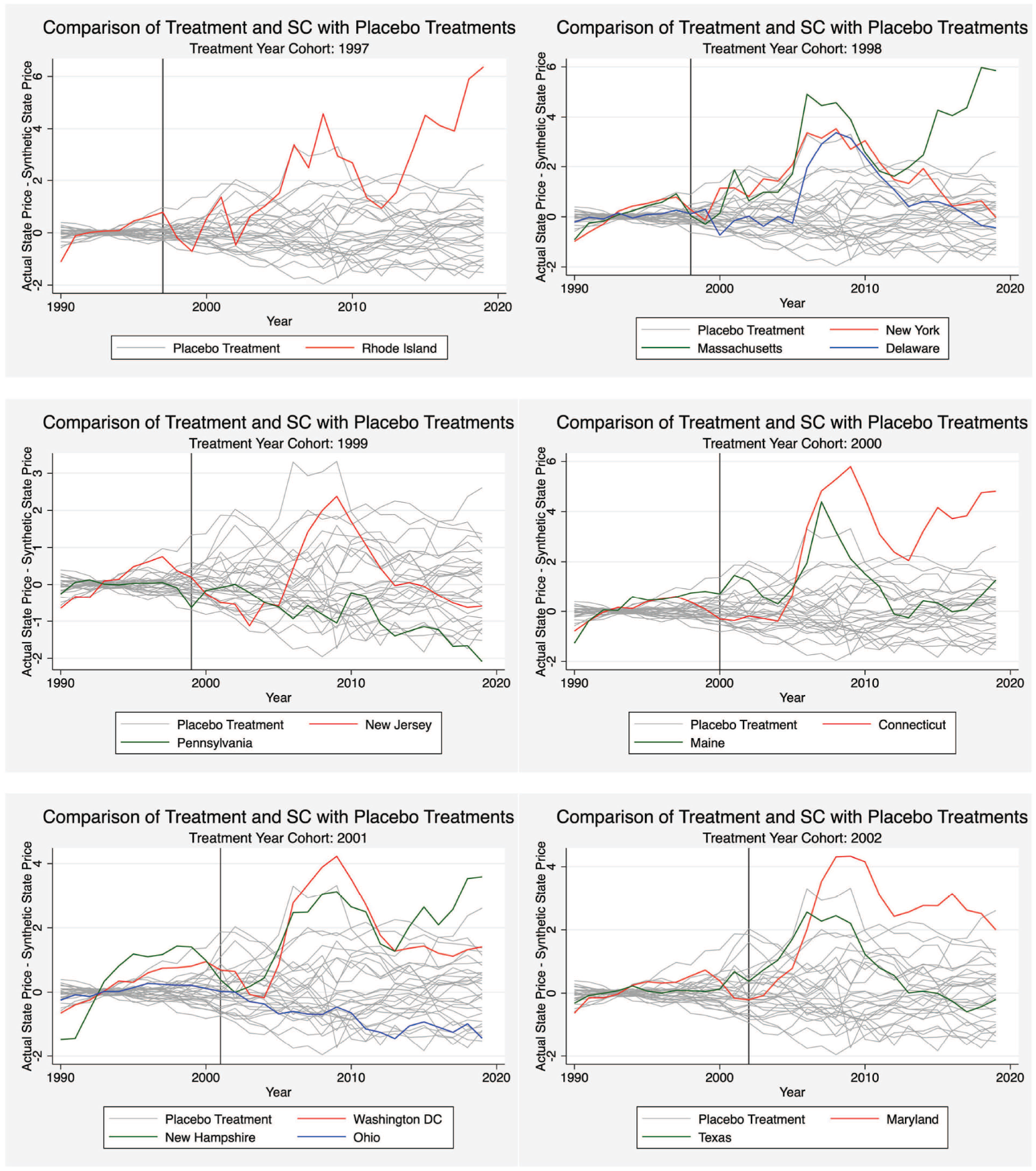
These results are shown graphically in Figure 2, where we show the difference in the electricity price observed in the treatment and control states compared to this difference in the placebo treatment states. ³⁴ Results are graphically presented six cohorts that correspond to the difference in the initial retail restructuring transition beginning dates shown in Table 1. Specifically, the six cohorts correspond to the retail restructuring beginning years from 1997 to 2002, with the number of states varying per year from one to three depending on the year.

Of the thirteen restructured states, ten exhibit the pattern of increased electricity prices relative to the synthetic control during the time period where natural gas prices were increasing (until approximately 2008) and then reconvergence. Notably, three of these states, Rhode Island, Massachusetts and Connecticut have seen a reversal in this trend, again experiencing increases in prices relative to controls despite natural gas prices nationally staying at historical lows. Two states, though, notably stand out as not being impacted in the same way as other states by restructuring; Pennsylvania and Ohio. This may be due to when the transition period ended for both states (2012 and 2011, respectively) that happened to coincide with when natural gas prices were already in decline (and during the transition retail prices increases were limited). These states were also uniquely positioned near historic increases in natural gas production.

Figure 2

Graphical Representation of Placebo Test

4.6.3 Bias from Staggered Treatment Adoption

Appendix Figures A9 and A10 present event study results from the stacked regressions. These event studies corroborate our event study results presented in Figures A4 and A5. Importantly, we do not find evidence of significant bias from staggered treatment adoption. Coefficients are only marginally higher from 5 to 10 years post-retail restructuring, compared with Figures A4 and A5, with significant differences between treated and control states becoming negligible by 12 years post-retail restructuring.

4.6.4 Falsification Outcomes

Appendix Table A4 presents results utilizing the two falsification outcomes, cooling degree days (CDDs) and gasoline consumption per person. We hypothesize that retail electricity market restructuring should not directly impact either of these outcomes. Of the twelve coefficient estimates shown in Table A4, eight are negative and four are positive and all are imprecisely estimated, confirming our hypothesis. Appendix Figure A8 shows these results graphically, alongside placebo tests of these falsification outcomes.

4.6.5 Parallel Pre-trends

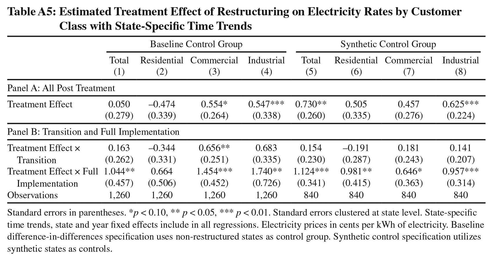
We follow Roth (2021) and perform diagnostics to determine what our likely power is against relevant pre-trend violations. We provide a visual diagnostic in the Appendix, Figure A11 of our estimated coefficients (in black), hypothesized trend (in red) and the expected coefficients conditional on passing the pre-test with our hypothesized trend (in blue). Although our pre-treatment coefficients show the potential for a pre-trend that we would have low power to detect, our post treatment coefficients follow a different pattern than we would expect if our true trend was the hypothesized trend and was not detected in pretesting (i.e., pre-trends passed). To formally allow for this potential violation in pre-trends, we provide estimates with differential trends by state in the Appendix, Table A6, to allow for the possibility that states were on differential growth trajectories with respect to electricity prices. We find that coefficients are largely unchanged from our baseline and synthetic control estimates in Table 3, however some estimates (particularly those for residential price effects in the baseline method) are statistically less precise.

5. Conclusions

In the mid-1990s, after decades of cost-of-service (COS) regulation, states began to transition generation assets from COS regulation to market-based remuneration and allow retail electricity customers the ability to choose their electric supplier (sometimes called “retail choice”). As noted, there have been previous studies estimating the impact of retail electricity market restructuring on retail prices, with mixed results. What is unique to this research is that the empirical analyses are based on detailed descriptions of each state’s restructuring timeline, including its transition period and date of full retail-restructuring implementation. This is an important distinction since states did not flash cut to full retail markets but phased them in over several years. Moreover, during the transition period states typically required incumbent utilities to discount retail prices. Such discounts should not be attributed to market forces, since they were the result of legislation, commission order, or negotiation. Another important characteristic of retail restructuring that is considered here is that each state passed legislation and commission implementation orders, began the transition period, and began retail market pricing at different times.

Conclusions of this research have significant policy implications. First, we do not find evidence that retail market restructuring has fulfilled its promise (made politically at the time) of reduced prices for retail customers. This result should not be interpreted to suggest that markets are not important in the electricity sector, but instead that retail restructuring specifically has not been associated with price reductions. This suggest that, on average, COS rate design has been reasonably successful at setting rates at a level where the allowed rate of return for the monopoly is approximately equal to the market cost of capital (see discussion of A-J model). Second, we do not find evidence that any customer class (i.e. residential, commercial, or industrial) benefited relative to others on average. This suggests that on average, states with COS regulation have also been reasonably successful at allocating costs across customer classes. Third we do find evidence that retail prices in restructured states move more in tandem with natural gas prices, the marginal fuel source of the time of analysis. Thus, there is evidence that these policies more quickly translated wholesale price signals to final customers. This aspect of retail restructuring might be viewed as either a benefit to the policy (i.e. transmitting price signals) or a cost (i.e. increasing the volatility of prices for customers).

Restructured states responded to the rapid retail electricity price increases observed during that period of increasing natural gas price with auctions or bidding processes to set the energy component of the retail price. This often, depending on the timing, was designed to blunt the impact that would have been felt by customers if the wholesale prices were simply passed through to the retail customers. Once natural gas prices began to fall around 2009, electricity prices began to converge between restructured and non-restructured states. Another policy response to higher natural gas and wholesale prices by states was, when possible, to restrict retail choice to only larger industrial and commercial customers. At the time of this writing (mid-2022), natural gas and wholesale prices are again elevated and our findings would suggest that restructured state retail prices would again respond more rapidly to wholesale price increases than COS states. Time will tell if this occurs.

We also test for whether retail restructuring facilitated the growth in renewable energy generation and find no such evidence. In fact, on average, restructured states had slower renewable energy growth than COS states, although we do not attribute any causal effect to this observation.

Although some will view this research as perhaps on balance favoring COS regulation over retail restructuring, we note a few important considerations. First, many COS states today are part of organized wholesale markets (i.e. ISOs and RTOs). Feedback from both utilities and regulators suggests that in these restructured states incorporated into organized wholesale markets, the day-to-day dispatch of generation assets is for all intents and purposes, similar to a restructured state. For COS states not in an organized wholesale market, dispatch is typically limited to the balancing area of the utility, not an entire region. There are opportunities for future research in this area. Second, historically some large industrial and commercial customers have advocated for retail access, as this allows them to engage in long-term contracts and other deals not available to large customers in COS states. Results from this research suggest that policy makers might be able to make retail access available to these larger customers, with little impact on prices of smaller residential and commercial customers. This is another area for future research.

Supplemental Material

sj-pdf-1-enj-10.5547_01956574.45.1.kros – Supplemental material for Retail Electricity Market Restructuring and Retail Rates

Supplemental material, sj-pdf-1-enj-10.5547_01956574.45.1.kros for Retail Electricity Market Restructuring and Retail Rates by Kenneth Rose, Brittany Tarufelli and Gregory B. Upton in The Energy Journal