Sage Journals: Discover world-class research

Abstract

This paper is the first to investigate the relationship between the energy efficiency of dwellings, measured by the energy performance certificate (EPC), and utility cost inclusion in rental prices. First, we investigate potential drivers behind the decision to include utility costs in rents. We find that labeled dwellings are more likely to include utility costs and that this likelihood is higher among energy-efficient dwellings than among inefficient dwellings. Next, we surprisingly find that utility costs seem to be under-capitalized in energy-inefficient dwellings. These results are confirmed with the counterfactual decomposition approach. Overall, the findings indicate that the EPC labeling policy may be important for both landlord and tenant decision-making and may enhance market efficiency.

Keywords

Energy performance certificates Utility costs Residential rental market Asymmetric information Housing policy

1. Introduction

Market failure has been widely researched in a range of markets such as labor, cars, finance, insurance and real estate. In markets characterized by imperfect information—i.e., markets in which one agent possesses information unknown to another—market efficiency may suffer. Agency theory explores the consequences of, and solutions to, adverse selection and moral hazard, where agents can behave in a self-serving manner because of the information asymmetry between them. For example, asymmetric information may often exist between landlords and tenants in the residential rental market. Energy performance certificates (EPCs) were introduced in the EU by the Energy Performance of Buildings Directive in 2002. An EPC provides information about a dwelling’s energy performance, measured on a scale from A (low expected energy consumption) to G (high expected consumption). The aim of the policy is to create economic incentives for agents in the real estate market to invest in environmentally friendly improvements that increase environmental sustainability. Much research has investigated the economic effects of the policy’s implementation, and there is a broad consensus that energy efficiency is capitalized in residential rents throughout Europe (e.g., Cajias, Fuerst, and Bienert 2019; Cajias and Piazolo 2013; Chegut et al. 2019; Dressler and Cornago 2017; Feige, Mcallister, and Wallbaum 2013; Fuerst and McAllister 2011; Hyland, Lyons, and Lyons 2013; Khazal and Sønstebø 2023, 2020; Kholodilin, Mense, and Michelsen 2017; Kok and Jennen 2012). By increasing awareness regarding the energy efficiency of dwellings through the EPC, issues with information asymmetry between landlords and tenants are expected to be mitigated.

The EPC scheme was fully implemented in Norway on July 1, 2010. It is managed by the Norwegian Water Resources and Energy Directorate and its daughter company for the reduction of energy consumption and the promotion of energy-efficient practices, Enova. Although the EPC is required to be included in all forms of marketing of for-sale and for-rent properties, a substantial share of properties remain unlabeled, especially in the rental market. A possible explanation for this is the lack of a proper penalty system and the regulators’ prioritization of more serious infractions when issuing fines, such as failed requirements regarding technical facilities and heating systems. Properties can be certified either by qualified experts who issue advanced and detailed certificates, or by a no-cost online self-assessment option that provide both advanced or simpler, less detailed certifications. The simple option is the most common certificate in the market, with about 90% of the total labeled dwellings. Although both options are effectively trust-based, the homeowner is legally responsible for the accuracy of the information provided. The certificate can be easily updated to reflect upgrades to the dwelling, and it is valid for ten years. Newer buildings will normally have at least a C rating because of the national standard technical requirements for construction of new buildings.

In the Norwegian residential rental market, tenants normally pay utility costs directly to the provider. However, some contracts have utility costs included as a fixed component in the rental price. In the US, Levinson and Niemann (2004) find that heat-included apartments tend to be more energy-efficient and that tenants in these apartments have higher energy consumption. Nevertheless, the premium of utility inclusion is less than the cost of energy consumption. Because landlords appear to value utility-included apartments despite the additional utility costs, the results may be partially explained by metering costs, economies of scale and signaling costs. Similarly, Maruejols and Young (2011) find that the intensity of total energy consumption is higher for Canadian households when the landlord pays for heating. Tenants of utility-included dwellings set the thermostat at a higher temperature during the day and are less likely to turn it down when the dwelling is unoccupied. Gillingham, Harding, and Rapson (2012) provide evidence of split incentives with results from California, where households that pay for heating are significantly more likely to adjust heating settings at night. Similarly, in the Swedish market, Elinder, Escobar, and Petré (2017) investigate a policy experiment conducted by a private housing company over a nine-year period from 2007 to 2015. They find that tenants reduced their electric energy consumption by 25% after being informed that they would shift from having utility costs included in the rent to paying the market price of energy. The reduction was immediate and permanent, indicating that individual metering and billing is effective in reducing energy consumption.

To the best of our knowledge, this paper is the first to study the relationship between utility cost inclusion, energy efficiency and rental prices, using a highly representative sample of approximately 670,000 observations from the Norwegian rental market between January 2011 and September 2019. We find that landlords of labeled dwellings are more likely to include utility costs in the rent. Moreover, the likelihood of utility cost inclusion is higher among energy-efficient dwellings than among energy-inefficient dwellings. Next, we investigate the impact of utility cost inclusion on rents. We find that including either electricity or heating costs yields rental premiums, and that the premium is of a reasonable magnitude compared to the expected energy cost. In an efficient market, we would expect the utility cost premium to reflect the cost of energy consumption. Consequently, energy-inefficient dwellings would have the highest premiums due to higher consumption for equal utility. However, we find that this is not the case. In general, utility cost premiums are lowest for non-green (D, E, F and G labels) dwellings, while no significant difference is found between green (A, B and C labels) and unlabeled utility cost premiums. These results are supported by the counterfactual decomposition approach.

Although we are unable to directly test competing mechanisms which may explain these results, reduced adverse selection and energy efficiency uncertainty may be contributing factors. If indeed they are the main drivers of our results and labelling does not entail substantial compliance and/or administrative costs, market efficiency may be enhanced by the added information provided by label adoption.

The paper is further organized as follows. Section 2 offers an overview of the data used in the analysis. In Section 3, we investigate the drivers behind the decision to include utility costs in the rent. In Section 4, we investigate the price effect of utility cost inclusion and discuss the results. Finally, we provide concluding remarks in Section 5.

2. Data and descriptive statistics

In this study, we use residential rental data obtained from Finn.no. The data contain posted monthly rents for residential dwellings, property characteristics, location (municipality and ZIP code) and variables for whether utility costs, i.e., electricity and heating, are included in the rent.¹ The sample contains approximately 670,000 observations, which cover the period from January 2011 through September 2019 and comprise the whole of Norway. The dataset is highly representative and contains information about dwellings located in all Norwegian counties, 98% of Norwegian municipalities and 74% of the country’s ZIP codes.

Although in Norway, the tenant normally pays utility costs directly to the provider, some contracts have utility costs included as a fixed component in the rental price. About 1.9% (N = 12,322) of the dwellings in our sample include utility costs in the rent. The average rental price for this subsample is about EUR 952, whereas the average rent for the subsample with no utility costs included is about EUR 928. The minimum and maximum rental prices for the whole sample are EUR 315 and EUR 3,600, respectively. Dwellings that include utility costs are, on average, smaller, have fewer bedrooms, and have a higher percentage of labeled dwellings, including both green-labeled dwellings and non-green dwellings. The dwellings that include utility costs have a lower percentage of unlabeled dwellings compared with those that do not include utility costs. This is reasonable because the energy label is assumed to be a good instrument to measure expected energy consumption; therefore, the absence of a label may reduce the likelihood of utility cost inclusion in rents.

The percentages of dwellings that have been rented out by professionals (real estate agents) with utility costs included and not included are about 7% and 13%, respectively. The highest share of dwellings that include utility costs is observed among apartments (78%), while the lowest share is among townhouses (0.6%). Table 1 provides comprehensive summary statistics for the dataset, and Figures A1 –A3 in the Appendix report the distribution of rents among green, non-green and unlabeled dwellings based on whether utility costs are included. Table A2 in the appendix shows a calculation of the expected monthly energy cost in relation to the average monthly rental price. The calculations suggest that on average, the energy cost for a 65 m² apartment without utility costs included amounts to 2.98% of the total rent.

Table 1

Summary statistics (January 2011–September 2019)

	Utility cost not included		Utility cost included
	Mean	St. Dev.	Mean	St. Dev.
Rental price (€)	928.10	365.22	951.54	359.02
Size (m²)	65.59	31.76	51.80	23.40
Number of bedrooms	1.70	0.99	1.31	0.79
Floor location	1.23	1.59	1.58	1.94
Age information (%)	0.66	8.11	0.26	5.09
Green (%)	7.59	26.48	16.43	37.05
Non-green (%)	8.44	27.80	9.75	29.66
Unlabeled (%)	83.97	36.69	73.83	43.96
Electricity included (%)			54.95	49.76
Heating included (%)			45.05	49.76
Furnished (%)	17.03	37.59	38.42	48.64
Centrally located (%)	46.02	49.84	68.60	46.41
Nice view (%)	24.85	43.21	35.11	47.73
Fireplace (%)	17.56	38.04	11.41	31.80
Janitor service included (%)	12.04	32.54	26.33	44.04
Hiking accessibility (%)	37.59	48.43	53.94	49.85
Security alarm (%)	04.92	21.63	7.40	26.18
No-smoking (%)	0.02	1.45	0.02	1.56
Public service accessibility (%)	0.21	4.56	1.14	10.64
Quiet area (%)	45.79	49.82	69.40	46.09
Garden (%)	0.57	7.55	0.10	3.12
Professionals (%)	12.89	33.51	6.81	25.19
Nonprofessionals (%)	87.11	33.51	93.19	25.19
Detached (%)	8.47	27.84	1.59	12.51
Bedsit (%)	11.08	31.38	19.27	39.44
Apartment (%)	75.81	42.82	77.76	41.59
Townhouse (%)	1.33	11.47	0.58	7.57
Semidetached (%)	3.31	17.88	0.81	8.97
2011 (%)	9.34	29.10	3.86	19.27
2012 (%)	10.05	30.06	7.01	19.27
2013 (%)	11.05	31.35	9.04	28.68
2014 (%)	13.10	33.74	11.84	32.31
2015 (%)	15.18	35.89	13.42	34.09
2016 (%)	14.01	34.71	18.61	38.92
2017 (%)	10.89	31.15	13.92	34.62
2018 (%)	09.38	29.16	13.41	34.07
2019 (%)	06.99	25.50	8.89	28.46
No. counties (% of Norway)	18 (100%)		18 (100%)
No. municipalities (% of Norway)	417 (98%)		416 (98%)
No. ZIP codes (% of Norway)	3,582 (74%)		3,580 (74%)
Sample size	657,572		12,322

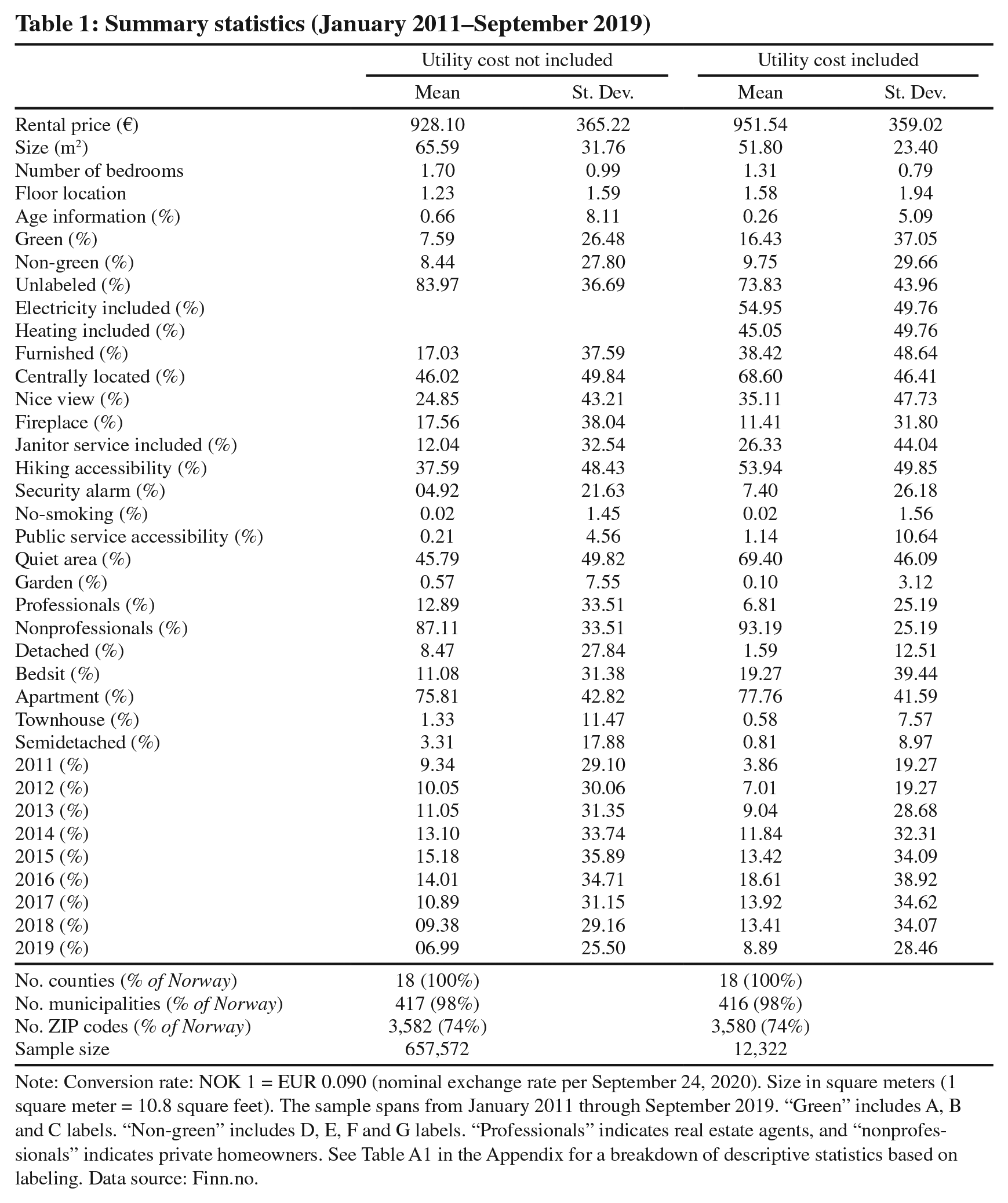
Note: Conversion rate: NOK 1 = EUR 0.090 (nominal exchange rate per September 24, 2020). Size in square meters (1 square meter = 10.8 square feet). The sample spans from January 2011 through September 2019. “Green” includes A, B and C labels. “Non-green” includes D, E, F and G labels. “Professionals” indicates real estate agents, and “nonprofessionals” indicates private homeowners. See Table A1 in the Appendix for a breakdown of descriptive statistics based on labeling. Data source: Finn.no.

3. Inclusion of utility costs

Several reasons may explain why some landlords include energy utility costs in the rents, including convenience or preference, economic and marketing purposes or because of shared utility costs in some apartment complexes. Figure 1 displays the proportion of dwellings with either electricity or heating included in the rent by dwelling type. Generally, electricity is the utility cost that is most often included, and the highest shares for both electricity and heating are found in apartments and bedsits. In building complexes with the same landlord, including utility costs may be more convenient than issuing electricity contracts for each new tenant in the complex. Moreover, it is easier for landlords to predict the expected energy consumption for smaller dwellings such as apartments and bedsits, which exhibit less variation in consumption. Regardless of dwelling type, the decision to include utility costs may also depend on marketing strategy (as an attractive feature for potential tenants) and on the building’s energy efficiency.

Figure 1

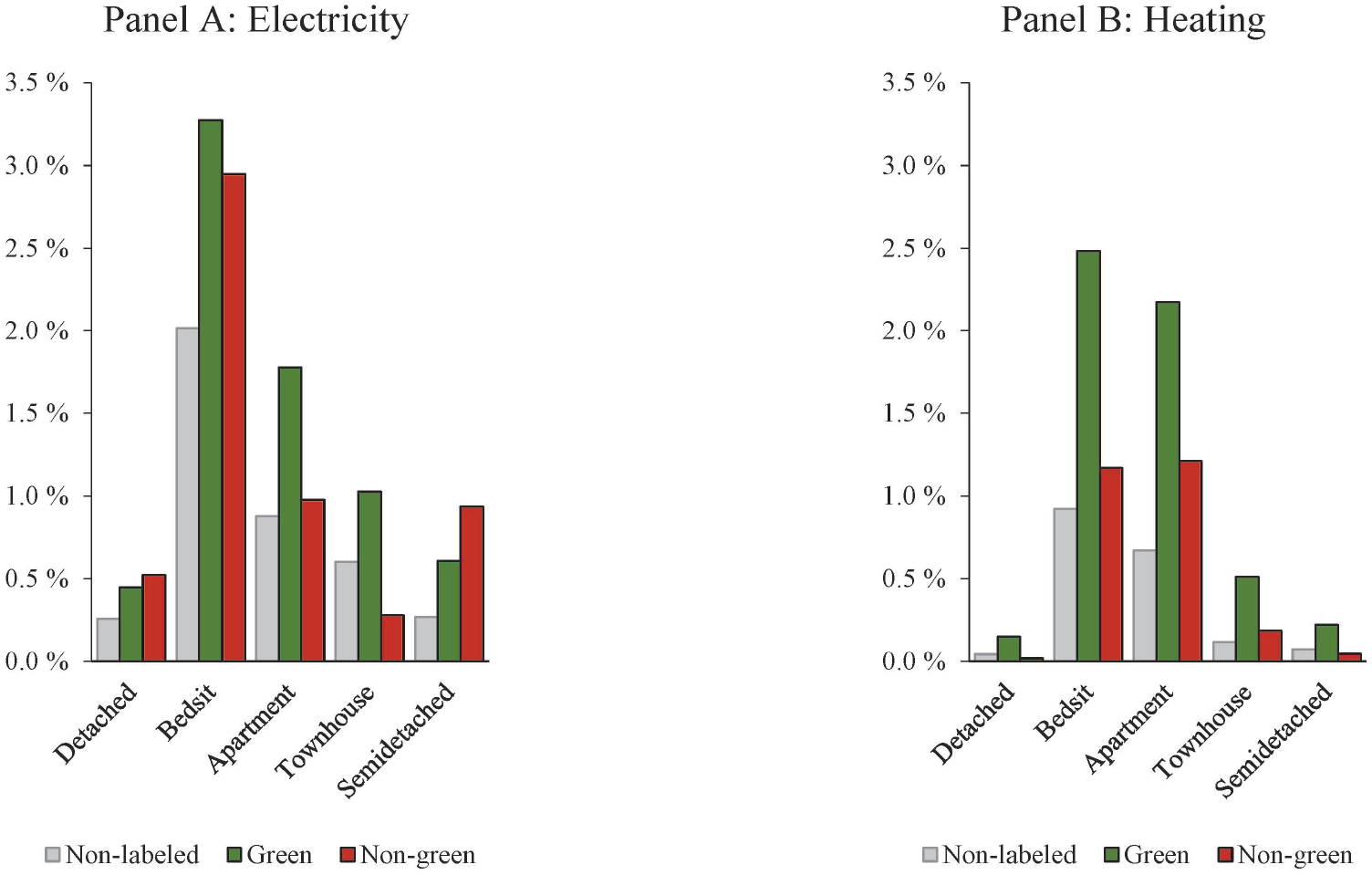
The share of dwellings with utility costs included in rent based on labels and dwelling types

In this subsection, we explicitly investigate the relationship between including utility costs, labeling, energy efficiency and rents. We begin by identifying the relationship between labels and the likelihood of utility cost inclusion by applying a logistic maximum likelihood estimation:

\frac{P U C_{i m z}}{1 - P U C_{i m z}} = e x p (Y_{i m z} β + φ_{m} + ρ_{z} + τ_{t} + e_{i m z})

(1)

where p_UC is the probability that the dummy variable UC is equal to 1. In the first two specifications, UC is defined as a dummy that takes the value 1 if either electricity or heating costs are included in the rental price of dwelling $i (i = 1, . . ., N)$ located in municipality $m (m = 1, . . ., M)$ and ZIP code $z (z = 1, . . ., Z)$ and 0 if the specific utility cost is not included. In the third specification, UC denotes a dummy variable that takes the value 1 if at least one of the utility costs is included. Y_imz is a vector of dwelling characteristics for the whole sample (reported in Table 1), including a dummy variable (Labeled) that takes the value 1 if the dwelling is energy labeled and 0 otherwise. We have also included controls for socioeconomic factors (the yearly logarithmic average age and logarithmic median income at the municipality level) and monthly logarithmic electricity prices/MW for each of the five Norwegian electricity price zones.² Considering only the labeled sample, energy-efficient dwellings are represented by a dummy (Green) that takes the value 1 if the dwelling is defined as green (A, B or C labels) and 0 otherwise. Alternatively, energy performance is represented by a continuous variable (Efficiency) ranging from 1 (G label) to 7 (A label). $β$ is a set of parameters of the independent variables estimated by maximum likelihood (ML). All time-invariant heterogeneity originating from municipality and ZIP codes is captured by the fixed effects $φ_{m}$ and $ρ_{z}$ , respectively. represents a vector of time-fixed effects for year, quarter and month, while e_imz is the error term, which is assumed to be uncorrelated with all the variables included in equation (1).

Table 2 displays three specifications of equation (1), where we estimate the inclusion of utility cost as a function of labels. To conserve space, Table 2 reports coefficients as odds ratios for several variables and as probabilities for the labeled and unlabeled groups only. The coefficient of the labeled group is significant and higher than 1 in all specifications, indicating that landlords of labeled homes are more likely to include utility costs in rents. Holding the other predictors constant, there is a higher likelihood of utility cost inclusion for smaller dwellings and dwellings with fewer bedrooms. Regarding dwelling types, there is a higher likelihood among bedsits, apartments and townhouses compared with detached and semi-detached houses. Furnished and centrally located dwellings are also associated with a higher likelihood of utility cost inclusion. Inclusion is more likely in municipalities with a higher average age, while municipalities with a higher median income are significantly more likely to include electricity alone. Electricity prices are significant only in the third specification, indicating that higher electricity prices are associated with a lower likelihood of inclusion. A potential explanation for this is that uncertainty regarding electricity bills increases when electricity prices are higher. Considering two otherwise equal dwellings, the likelihood of including utility costs is higher for the labeled one, indicating that the label itself is an important tool for the landlord to calculate the expected energy consumption.

Table 2

Utility cost inclusion decision and labels

Odds ratio	Electricity	Heating	Utility
Labeled	1.2365***	1.7157***	1.4710***
Labeled	(6.62)	(16.32)	(17.00)
Size	0.9921***	0.9888***	0.9908***
Size	(–8.08)	(–9.79)	(–12.40)
Number of bedrooms	0.8254***	0.9602	0.8776***
Number of bedrooms	(–7.49)	(–1.51)	(–7.01)
Bedsit	2.2816***	6.4373***	2.7872***
Bedsit	(8.78)	(8.53)	(12.41)
Apartment	1.5664***	6.3576***	2.1951***
Apartment	(5.25)	(8.72)	(10.22)
Townhouse	1.7328***	2.5974**	1.8016***
Townhouse	(3.45)	(2.75)	(4.14)
Semidetached	1.0531	1.3995	1.0356
Semidetached	(0.37)	(1.07)	(0.28)
Furnished	2.7516***	1.5069***	2.1843***
Furnished	(36.89)	(12.33)	(37.59)
Centrally located	1.2611***	1.4453***	1.3352***
Centrally located	(7.00)	(8.75)	(11.23)
Age	4.0251***	7.4175***	3.6097***
Age	(3.89)	(4.76)	(4.74)
Income	1.4352**	0.9080	1.1036
Income	(2.82)	(–0.60)	(0.99)
Electricity prices	0.9348	0.9369	0.9347*
Electricity prices	(–1.56)	(–1.31)	(–2.08)
Controls	✓	✓	✓
Probability
Labeled	0.0119***	0.0114***	0.0245***
Labeled	(36.45)	(37.56)	(54.17)
Unlabeled	0.0097***	0.0067***	0.0169***
Unlabeled	(71.62)	(58.23)	(94.41)
Observations	647,043	647,182	647,182
Chi squared stat.	7,355.288	6,015.911	11,985.709
Pseudo R²	0.078	0.094	0.0876

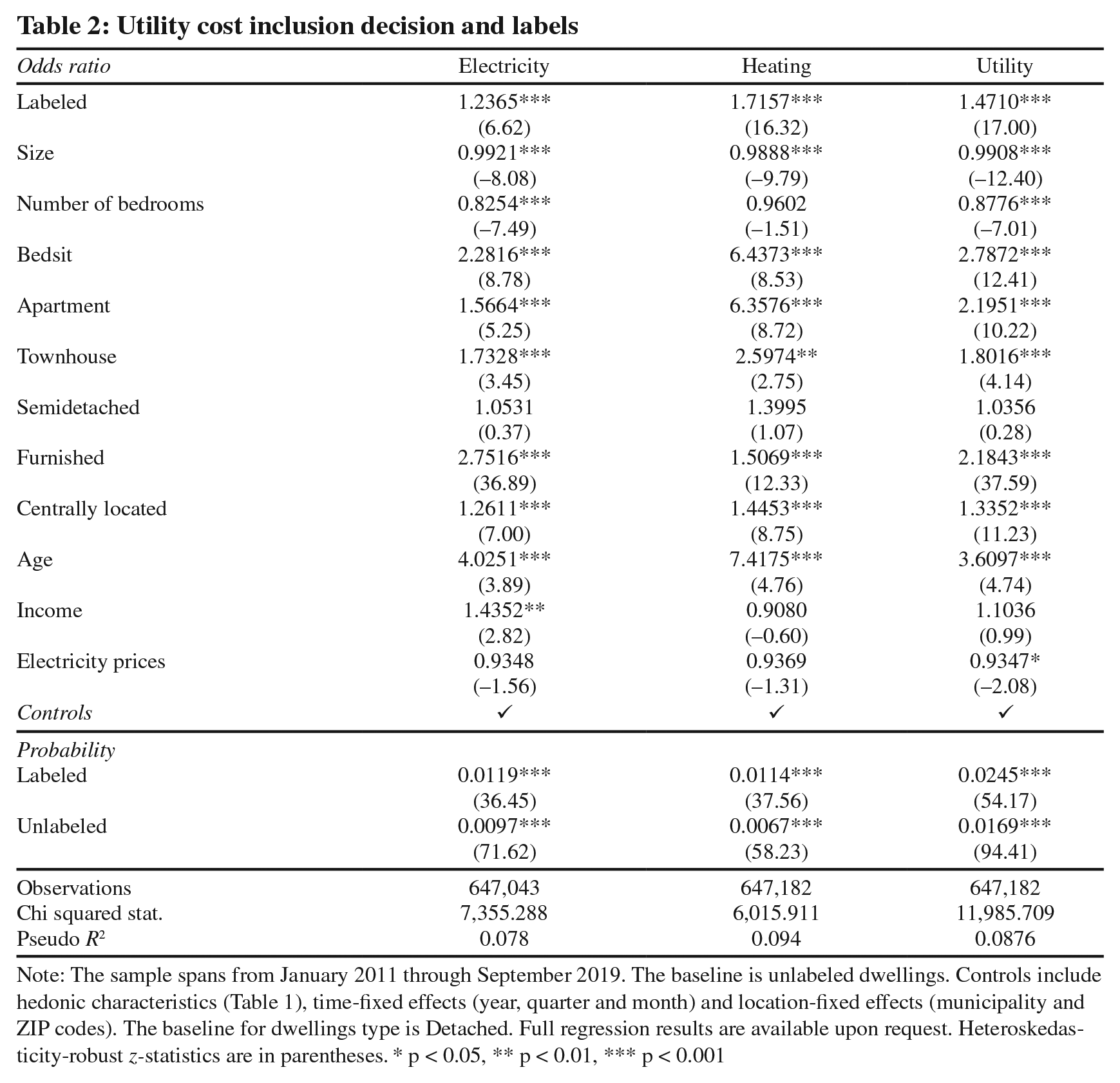
Note: The sample spans from January 2011 through September 2019. The baseline is unlabeled dwellings. Controls include hedonic characteristics (Table 1), time-fixed effects (year, quarter and month) and location-fixed effects (municipality and ZIP codes). The baseline for dwellings type is Detached. Full regression results are available upon request. Heteroskedasticity-robust z-statistics are in parentheses. * p < 0.05, ** p < 0.01, *** p < 0.001

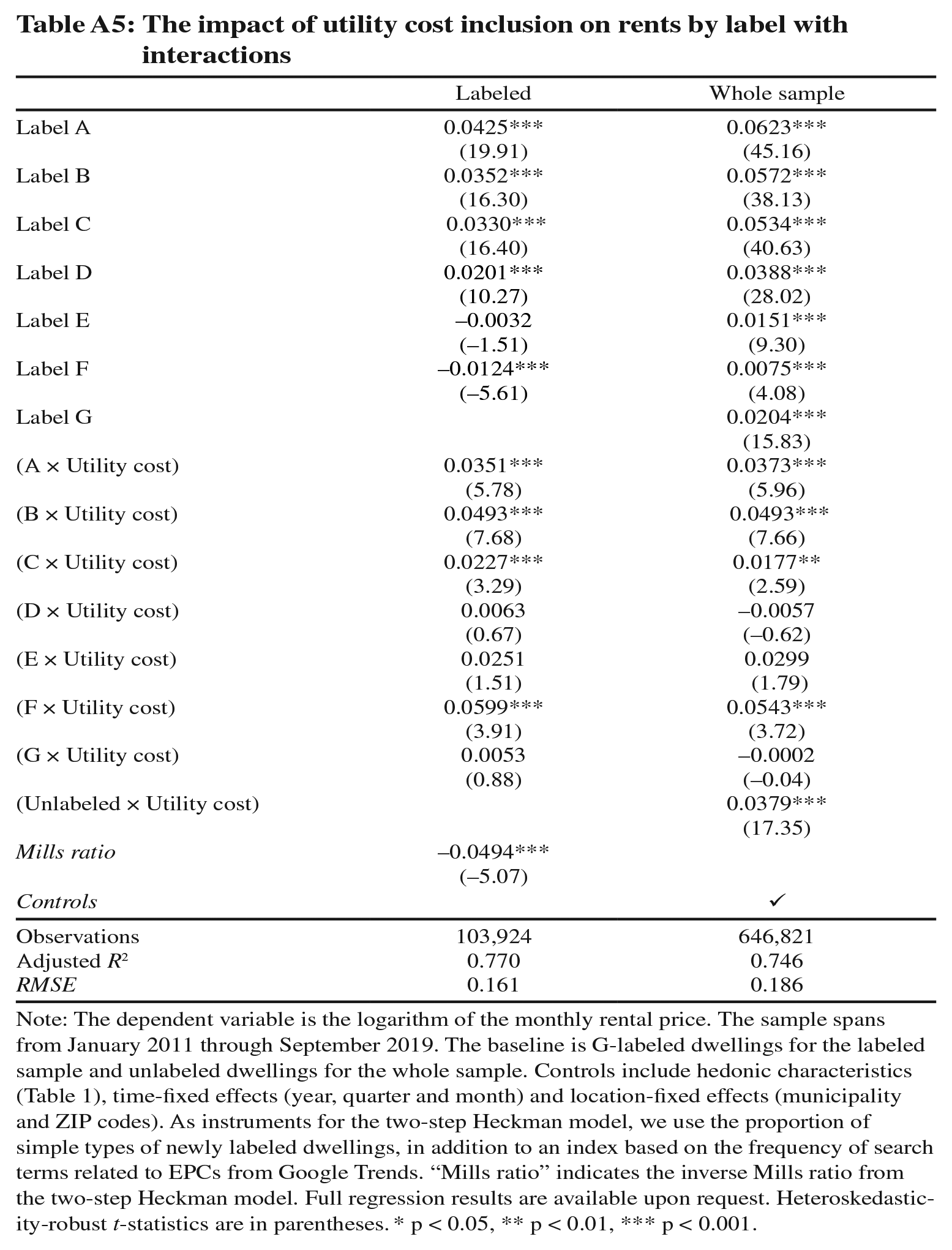
Up to this point, we have investigated the likelihood of utility cost inclusion in relation to labels without considering dwellings’ energy efficiency. In Table 3, we re-estimate equation (1) using the subsample of labeled dwellings where utility cost inclusion is a function of either the dummy variable of green labeled homes (Green) or the continuous variable of energy efficiency (Efficiency). In all specifications, the green coefficients are positive and highly significant, indicating that landlords of green homes are more likely to include utility costs in rent compared with landlords of non-green homes. The results from Table 3 also demonstrate that the likelihood of including utility costs in rents increases with dwellings’ energy efficiency, and that the likelihood of including heating is the highest. The coefficient of Efficiency indicates that a one-letter improvement (e.g., from C to B) increases the likelihood of utility cost inclusion in rents. This is also supported by the estimated results for each label in Table A5 in the Appendix, with the corresponding probabilities displayed in Figure 2. Energy-efficient homes’ higher likelihood of utility cost inclusion may be related to lower uncertainty regarding energy consumption.

Table 3

Utility cost inclusion and energy efficiency

Odds ratio	Electricity		Heating		Utility
Green	1.2931***		1.8573***		1.5874***
Green	(4.24)		(10.40)		(11.01)
Efficiency		1.0798***		1.1905***		1.1405***
Efficiency		(5.08)		(10.84)		(12.04)
Controls	✓	✓	✓	✓	✓	✓
Probability
Green	0.0150***		0.0192***		0.0359***
Green	(28.31)		(29.90)		(42.90)
Non-green	0.0116***		0.0105***		0.0231***
Non-green	(22.31)		(23.01)		(33.10)
Observations	105,175	105,175	105,271	105,271	105,271	105,271
Chi squared stat.	838.104	827.071	1253.381	1255.249	1691.169	1689.160
Pseudo R²	0.053	0.053	0.081	0.083	0.066	0.067

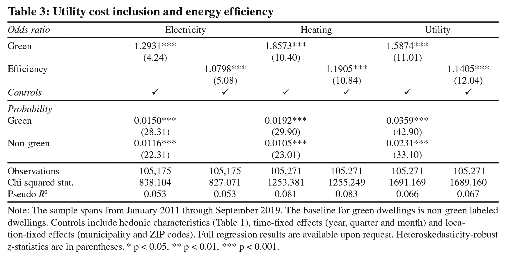
Note: The sample spans from January 2011 through September 2019. The baseline for green dwellings is non-green labeled dwellings. Controls include hedonic characteristics (Table 1), time-fixed effects (year, quarter and month) and location-fixed effects (municipality and ZIP codes). Full regression results are available upon request. Heteroskedasticity-robust z-statistics are in parentheses. * p < 0.05, ** p < 0.01, *** p < 0.001.

Figure 2

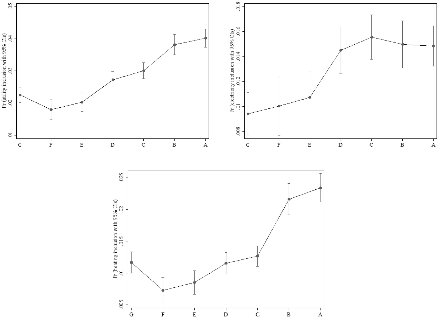
The probability of utility cost inclusion in rents

4. The impact of utility costs on rents

In this section, we analyze the relationship between efficiency, energy consumption, and rents. Assuming rational actors with perfect information, the rental price P_UC with included utility cost can be expressed as

P_{u c} = P_{0} + E [c],

(2)

where P₀ is the initial rental price, $E [c],$ is the expected energy consumption cost for the included utility, and the premium is defined as $δ = E [c] > 0 .$ ³ Because inefficient dwellings have higher expected energy consumption, $E [c_{n o n - g r e e n}] > E [c_{g r e e n}],$ the premium is likely to be higher for these dwellings, $δ_{n o n - g r e e n} > δ_{g r e e n} .$ Furthermore, because unlabeled dwellings are, on average, unlikely to be as efficient as green dwellings, $E [c_{n o n - l a b e l e d}] > E [c_{g r e e n}],$ and because unlabeled dwellings are either inefficient (equal to non-green) or contain both inefficient and efficient (equal to green) dwellings, $E [c_{n o n - g r e e n}] \geq [c_{n o n - l a b e l e d}],$ we expect that the utility cost premium of non-green dwellings is greater than or equal to that of unlabeled dwellings, and that the premium of unlabeled dwellings is greater than that of green dwellings:

δ_{n o n - g r e e n} \geq δ_{n o n - l a b e l e d} > δ_{g r e e n} .

(3)

4.1 Hedonic approach

To investigate how utility cost inclusion influences rental prices, we employ a hedonic real estate valuation framework (Rosen 1974) that is widely used in economic research. We develop a semi-log hedonic HDFE model that relates the log of rental prices to utility costs, energy efficiency, dwelling attributes (Table 1), location, and time:

L o g (p r i c e_{i m z}) = U C_{i m z} δ + Y_{i m z} β + φ_{m} + ρ_{z} + τ_{t} + u_{i m z},

(4)

where the dependent variable is the natural logarithm of the rental price of dwelling i located in two locational levels (municipality and ZIP code). UC_imz is the variable of interest and represents a dummy for utility costs that takes the value 1 if electricity costs are included in rents and 0 otherwise. In a second specification, UC_imz represents heating costs. Finally, in a third specification, UC_imz takes the value 1 if at least one utility cost is included in the rent and 0 otherwise. $δ$ is the corresponding coefficient estimated by OLS to identify and quantify the impact of utility cost inclusion on rents, while u_imz is the error term assumed to be independent of all explanatory variables; the remainder is defined in equation (1).

Further, it is necessary to consider that labeling may be subject to selection bias. For example, landlords of efficient dwellings may wish to market them toward tenants with green preferences, and may therefore be less likely to voluntarily certify if the expected energy efficiency is low. This issue has been addressed in the previous literature (e.g., Brounen and Kok 2011; Hyland, Lyons, and Lyons 2013; Khazal and Sønstebø 2023, 2020; Olaussen, Oust, and Solstad 2017), and we therefore apply the two-step Heckman selection approach when estimating equation (4). We use two instruments in the first-stage Heckman probit model, where the dependent variable is a dummy taking the value 1 if the dwelling is labeled and 0 otherwise.⁴ First, we use the proportion of simple types of new labeled dwellings per month at the municipality level to the corresponding total number of new labels, thus controlling for landlords’ self-selection of certificate type. Second, we create an index based on the monthly frequency of search words related to EPCs from Google Trends.⁵ In the second step, we include robust estimates of the inverse Mills ratio obtained from the first step when estimating equation (4), using the subsample of labeled dwellings.

In Table 4, we estimate equation (4) using the whole sample as well as the labeled and unlabeled subsamples. In columns 1 and 2, the coefficients of green labeled dwellings are positive and highly significant, indicating that energy-efficient homes are associated with 5.8% and 3.2% premiums compared with unlabeled and non-green dwellings, respectively. For the non-green dwellings in column 1, the premium is about 2.3% compared with unlabeled dwellings. These results are consistent with the existing literature (e.g., Khazal and Sønstebø 2023). Next, the results provide evidence that rents that include utility costs are associated with a premium, as expected. When estimating the whole sample, the coefficients of electricity and heating are positive and significant, and the inclusion of both electricity and heating costs yields similar premiums of about 3.2–3.5%.

Table 4

The impact of utility cost inclusion on rents

Whole sample		Labeled	Unlabeled
Green	0.0575***	0.0322***
Green	(68.27)	(25.76)
Non-green	0.0225***
Non-green	(27.88)
Electricity	0.0354***	0.0269***	0.0374***
Electricity	(13.30)	(5.17)	(12.09)
Heating	0.0320***	0.0277***	0.0329***
Heating	(13.43)	(7.87)	(10.72)
Electricity prices	–0.0074***	–0.0095***	–0.0067***
Electricity prices	(–9.26)	(–5.30)	(–7.16)
Age	2.4169***	1.9889***	2.6175***
Age	(39.73)	(12.32)	(35.75)
Income	2.5285***	2.6026***	2.6035***
Income	(138.45)	(59.93)	(126.67)
Mills ratio		–0.0508***	0.0562***
Mills ratio		(–5.21)	(3.77)
Controls	✓	✓	✓
Sample size	646,821	103,924	532,106
Adjusted R²	0.746	0.769	0.734
RMSE	0.186	0.161	0.190

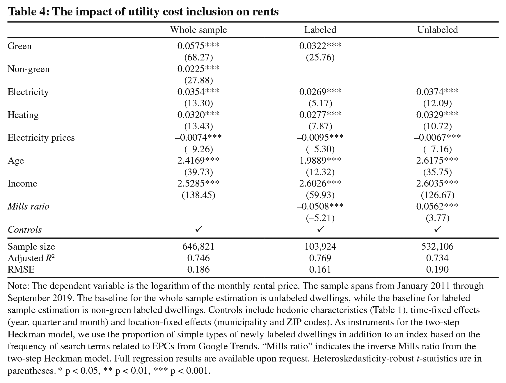
Note: The dependent variable is the logarithm of the monthly rental price. The sample spans from January 2011 through September 2019. The baseline for the whole sample estimation is unlabeled dwellings, while the baseline for labeled sample estimation is non-green labeled dwellings. Controls include hedonic characteristics (Table 1), time-fixed effects (year, quarter and month) and location-fixed effects (municipality and ZIP codes). As instruments for the two-step Heckman model, we use the proportion of simple types of newly labeled dwellings in addition to an index based on the frequency of search terms related to EPCs from Google Trends. “Mills ratio” indicates the inverse Mills ratio from the two-step Heckman model. Full regression results are available upon request. Heteroskedasticity-robust t-statistics are in parentheses. * p < 0.05, ** p < 0.01, *** p < 0.001.

In the labeled subsample in column 2, the premiums are about 2.7% for both utility cost types. Considering the unlabeled sample in column 3, premiums of about 3.7% and 3.3% are observed for the inclusion of electricity costs and heating costs, respectively. Although the utility cost premiums of unlabeled dwellings seem to be higher relative to those of labeled dwellings, only the electricity cost premium is significantly higher. The magnitude of the premiums seem reasonable considering the expected utility cost calculations in Table A2.

The coefficients of age and income are positive and significant, indicating higher rents in municipalities with higher average ages and median incomes. Electricity prices have negative and significant coefficients, indicating that rents are lower during periods of higher electricity prices. The coefficient of the selection variable, the inverse Mills ratio, is significant, indicating that both labeled and unlabeled subsamples are subject to selection bias. Whereas the negative coefficient in the labeled sample implies that the error terms in the selection equation and equation (4) are negatively correlated, the opposite is observed for the unlabeled sample. The F-statistic from the first-stage probit estimation is 11.73, which is higher than the rule of thumb of 10, providing evidence in favor of the relevance condition of the Heckman selection model. Due to the inclusion of two instruments, we can partially test for the exogeneity condition by applying the Sargan overidentification test. The J-statistics for the Sargan tests are 0.431 and 5.749 for the labeled and unlabeled estimations, respectively. Because these statistics are lower than the critical value of 6.634, they provide evidence supporting the instruments’ exogeneity condition.

However, the results from Table 4 do not consider the energy efficiency of labeled dwellings. Therefore, they are insufficient to provide a detailed understanding of the underlying mechanism behind the premiums. To identify and quantify the joint impact of utility costs and efficiency on rents, we include interaction variables for both green and non-green labels with utility costs (at least one of electricity or heating) using the labeled subsample. Additionally, we include an interaction term for unlabeled dwellings with utility costs when estimating the whole sample.

The results in Table 5 provide evidence that dwellings with the same energy efficiency are associated with a premium if utility costs are included in rents. The utility cost premium is 2.9% and 3.5% for the labeled and whole sample, respectively. Compared with the calculations in Table A2, we find that the premiums are in the expected range. When considering energy efficiency, the utility cost premium for green dwellings is about 3.6%, whereas the premium is about 1.1–1.6% for non-green dwellings. Considering the whole sample, the premium of utility cost inclusion among unlabeled dwellings is 3.8%; this premium is not significantly higher than that of green dwellings. The findings are supported by the results in Tables A4–A5 in the Appendix, where we run the labeled subsample with the efficiency variable and for each label individually (instead of the green and non-green dummies). Since the utility cost premium of energy-inefficient dwellings is lower than that of energy-efficient dwellings, the results are inconsistent with equation (3) and suggests two possibilities: the energy consumption cost is either not fully capitalized in the non-green dwelling rents and/or is overcapitalized in the green and unlabeled dwelling rents. Comparing with the calculations in Table A2, both possibilities seem plausible.

Table 5

The impact of labels and utility costs on rents

Labeled		Whole sample
Green	0.0321***	0.0316***	0.0575***	0.0575***
Green	(25.73)	(25.03)	(68.20)	(67.08)
Non-green			0.0224***	0.0230***
Non-green			(27.87)	(28.36)
Utility cost	0.0285***		0.0348***
Utility cost	(9.25)		(19.24)
(Green × UC)		0.0359***		0.0360***
(Green × UC)		(9.51)		(9.44)
(Non-green × UC)		0.0159**		0.0106*
(Non-green × UC)		(3.07)		(2.06)
(Unlabeled × UC)				0.0377***
(Unlabeled × UC)				(17.29)
Mills ratio	–0.0509***	–0.0508***
Mills ratio	(–5.22)	(–5.21)
Controls	✓	✓	✓	✓
Sample size	103,924	103,924	646,821	646,821
Adjusted R²	0.769	0.770	0.746	0.746
RMSE	0.1612	0.161	0.186	0.186

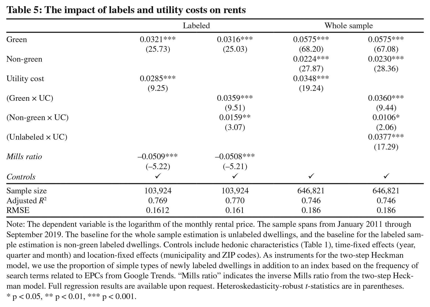
Note: The dependent variable is the logarithm of the monthly rental price. The sample spans from January 2011 through September 2019. The baseline for the whole sample estimation is unlabeled dwellings, and the baseline for the labeled sample estimation is non-green labeled dwellings. Controls include hedonic characteristics (Table 1), time-fixed effects (year, quarter and month) and location-fixed effects (municipality and ZIP codes). As instruments for the two-step Heckman model, we use the proportion of simple types of newly labeled dwellings in addition to an index based on the frequency of search terms related to EPCs from Google Trends. “Mills ratio” indicates the inverse Mills ratio from the two-step Heckman model. Full regression results are available upon request. Heteroskedasticity-robust t-statistics are in parentheses. * p < 0.05, ** p < 0.01, *** p < 0.001.

4.2 Counterfactual decomposition approach

Another way to investigate energy efficiency and utility cost inclusion is the counterfactual decomposition technique, popularized by Blinder (1973) and Oaxaca (1973). The Blinder–Oaxaca decomposition technique is especially useful for identifying and quantifying the separate contributions of group differences to measurable characteristics. It is often used to identify wage gaps originating from gender and race discrimination in labor markets. Consider two groups of landlords in the rental market: Group 1 includes utility costs in rents, and Group 2 does not include utility costs. The linear hedonic model for the two groups can be presented as follows:

p_{i} = Y_{i}^{'} β_{i} + ϵ_{i} for i \in {1, 2},

(5)

where p_i is the natural logarithm of the rental price, Y is a vector containing the hedonic characteristics of the dwelling, $β$ contains the slope parameters and the intercept, and $ϵ_{i}$ is the error term. We assume that, on average, Group 1 and Group 2 have different valuations for dwellings with the same attributes due to the inclusion of utility costs. With $E (p_{i}) = p_{i}, E (β_{i}) = β_{i}$ and $E (ϵ_{i}) = 0$ by assumption, the difference in the conditional expectation of dwelling rental prices between the two groups can be formulated as follows:

D = E (p_{1}) - E (p_{2}) = [E {(Y_{1})}^{'} β_{1}] - [E {(Y_{2})}^{'} β_{2}]

(6)

Further, we assume that $β *$ is a set of benchmark coefficients that should be used to determine the contribution of the differences in the predictors. The outcome difference represented in equation (6) can be rearranged as follows:

D = {[E (Y_{1}) - E (Y_{2})]}^{'} β * [E {(Y_{1})}^{'} (β_{1} - β^{*}) + E {(Y_{2})}^{'} (β^{*} - β_{2})] .

(7)

Equation (7) is the twofold Blinder–Oaxaca decomposition for linear regression models, which divides the outcome differential into two components. The first portion on the left-hand side of equation (7) is the “explained” component—i.e., the portion of the aggregate group difference in rental price that is explained by the differences in the mean value of the predictors. Equation (7) is formulated from the viewpoint of Group 2; the coefficient of the explained part measures the expected change in Group 2’s mean outcome if Group 2 had the same predictor levels as Group 1. The next term represents the “unexplained” portion, which is due to differences in the coefficient estimates, including those of the intercepts.⁶ This portion can be considered the outcome differential—due to the expected energy consumption costs and other factors related to the premium of utility cost inclusion—that would remain even if Group 2 had the same mean levels of the predictors as Group 1.⁷ See Jann (2008) for a detailed explanation of the methodology and implementation.

We apply the Blinder–Oaxaca decomposition technique, accounting for labeling and energy efficiency by estimating the subsamples of green, non-green and labeled dwellings separately (Table 6). For the green subsample in column (1), the differential coefficients indicate that the average logarithmic rental price is 2.8% higher for dwellings that include utility costs in rent. The decomposition coefficient of the explained component shows that no significant part of the difference can be attributed to the model predictors; the total difference between the two green labeled groups is due only to the positive and significant unexplained portion.

Table 6

Blinder–Oaxaca decomposition results

	Green	Non-green	Unlabeled
	(1)	(2)	(3)
Differential:
UC included	9.2926***	9.3495***	9.1667***
UC included	(1,273.36)	(1,000.39)	(2,425.36)
UC not included	9.2646***	9.3496***	9.1478***
UC not included	(6,252.47)	(6,315.05)	(18,055.69)
Difference	0.0280***	–0.0002	0.0189***
Difference	(3.76)	(–0.02)	(4.96)
Decomposition:
Explained	–0.0099	–0.0251**	–0.0201***
Explained	(–1.54)	(–2.99)	(–5.98)
Unexplained	0.0379***	0.0249***	0.0390***
Unexplained	(9.63)	(4.53)	(17.00)
Sample size	50,201	55,070	541,911

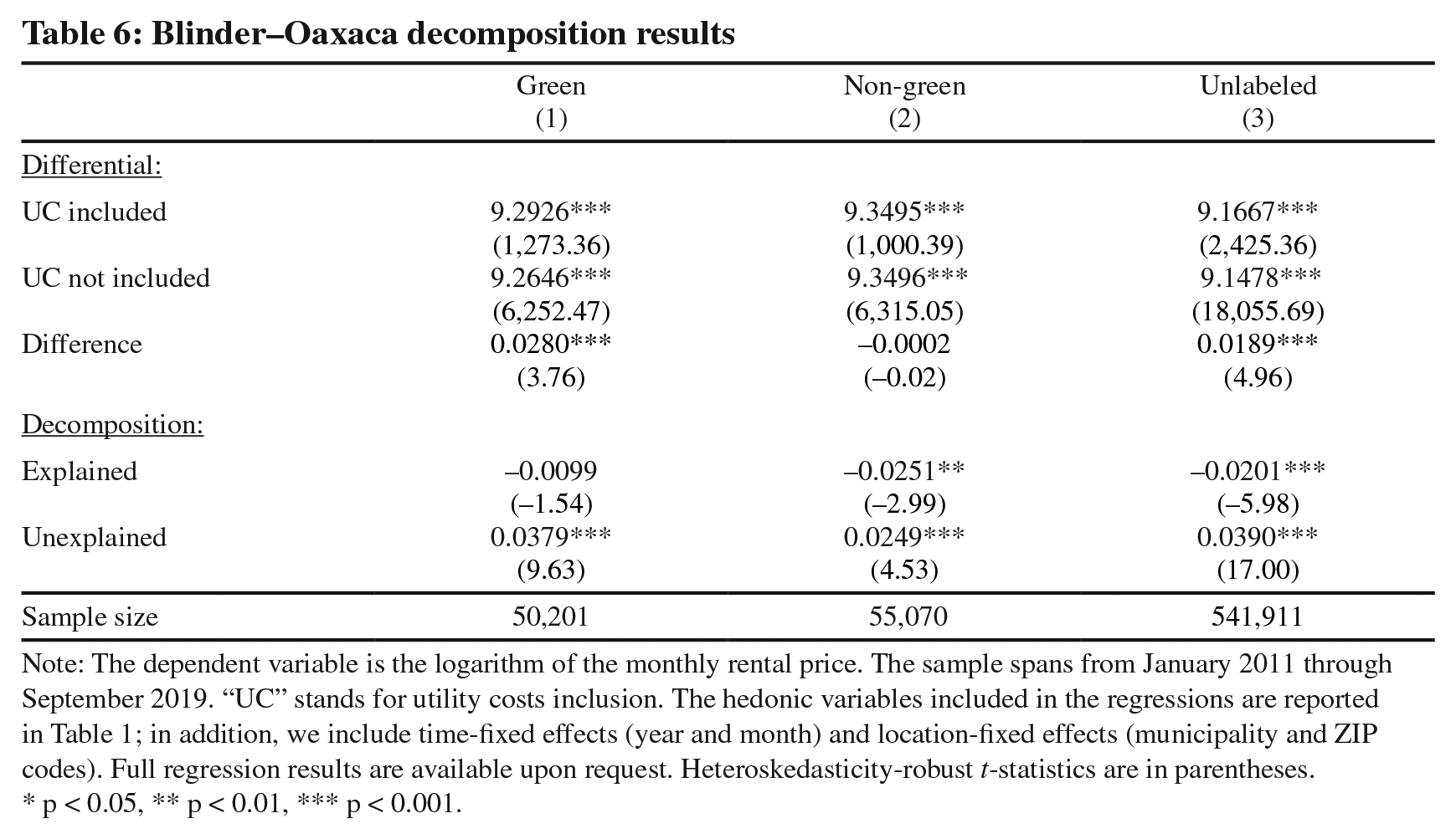
Note: The dependent variable is the logarithm of the monthly rental price. The sample spans from January 2011 through September 2019. “UC” stands for utility costs inclusion. The hedonic variables included in the regressions are reported in Table 1; in addition, we include time-fixed effects (year and month) and location-fixed effects (municipality and ZIP codes). Full regression results are available upon request. Heteroskedasticity-robust t-statistics are in parentheses. * p < 0.05, ** p < 0.01, *** p < 0.001.

Considering the subsample of non-green dwellings in column (2), there is no significant price difference between the two groups (UC included and UC not included). However, the decomposition coefficients show that the explained and unexplained components are both significant with different signs and thus balance out. The negative significant Explained coefficient indicates that adjusting Group 1’s (dwellings with utility costs included) predictors to the same levels as Group 2 (dwellings without utility costs included) would increase Group 1’s rents by 2.5%. A gap of 2.5% remains unexplained.

In column (3), we consider the unlabeled subsample and find that the price difference is positive and significant. As in the non-green estimations, the explained component of the difference is negative and significant, while the price difference is driven by the greater magnitude of the significant unexplained component. These results are consistent with the interaction terms between utility inclusion and the green, non-green and unlabeled categories in Table 5.

4.3 Discussion of potential explanations

The counterintuitive results may be explained by other factors, some of which may be related to asymmetric information and uncertainty. While hard to disentangle with the available data at hand, we shortly discuss the potential effects. Because landlords can predict energy consumption more accurately than new tenants, they can take advantage of the absence of labeling and assign higher premiums when utility costs are included; thus, there may be an adverse selection premium. An additional type of asymmetric information exists after the contract is signed: landlords have less control over tenants’ energy consumption levels because the latter have no (or little) incentive to save energy when the marginal cost of energy consumption is zero. Therefore, tenants may use more energy when the cost of utility is included in the rent (Myers 2020). Consequently, the landlord may assign a moral hazard risk premium for the potential hidden action of the tenant. Furthermore, if sufficient knowledge about a dwelling’s energy efficiency is unavailable, the landlord is less likely to accurately predict the expected energy consumption and may therefore assign an efficiency uncertainty premium. Although the landlord can use previous tenants’ energy consumption as an indicator, new tenants are likely to have different preferences. Therefore, the problems of moral hazard and uncertainty cannot be completely eliminated. Additionally, there may exist a marketing risk aversion discount; some landlords may be willing to accept a loss on the inclusion of utility costs to attract more potential tenants and thus reduce time on market and transaction costs (Cajias, Fuerst, and Bienert 2019).

For green dwellings that include utility costs, the label provides information for both landlords and tenants that could reduce the risk of adverse selection and efficiency uncertainty. We expect the effects of moral hazard to be lower for efficient dwellings, and because the high energy efficiency raises the attractiveness of the dwelling, the need for a marketing risk aversion discount could be low. However, landlords of energy efficient dwellings may specifically market utility cost-included dwellings toward individuals with green preferences, which could allow them to charge a higher premium while being subject to a lower risk of moral hazard in the form of over-consumption.

Since unlabeled dwellings are, on average, unlikely to be as efficient as green dwellings, there could be both a moral hazard premium and a marketing risk aversion discount assigned to the rent. At the same time, the absence of labeling may increase the possibility of both adverse selection and uncertainty. However, if these or other effects are present, they seem to cancel out since the utility cost premium is not significantly different from that of green dwellings.

The premium for non-green dwellings is harder to explain. Since the effects of adverse selection and uncertainty are somewhat mitigated by the labeling information, we expect that moral hazard and marketing contributes more to the estimated premium. However, the potential moral hazard premium should be higher for non-green dwellings regardless of whether tenants with green preferences sort into energy efficient dwellings or the relative likelihood of them engaging in moral hazard behaviour. This means that in order to observe the low utility cost premium in our findings, other premium-reducing factors such as the marketing discount must be relatively substantial, or other factors may be at play.

Naturally, there may be other factors involved that we are not able to control for with the data available in this paper, such as within zip-code correlation between energy efficiency and/or utility cost inclusion and unobservable socio-economic demographics. Further research could be aided using survey data in order to investigate self-selection into the EPC-program and the reliability of the self-assessment certification.

5. Conclusion and implications

This paper is the first to investigate the relationship between utility cost inclusion, energy efficiency and rental prices. First, we investigate potential drivers behind the decision to include utility costs in rents. We find that the landlords of labeled dwellings are more likely to include utility costs, which may be explained by higher uncertainty regarding energy efficiency and consumption among unlabeled dwellings. Further, the likelihood of utility cost inclusion is higher among more energy-efficient (green) dwellings than among energy-inefficient (non-green) dwellings. This may be related to the calculation of expected energy consumption, because varying tenant preferences for energy consumption have smaller financial impacts on dwellings with higher energy performance.

We also investigate the impact of utility cost inclusion on rents. After controlling for a vast number of attributes and socio-economic factors, location and time fixed effects, and potential selection bias using the two-step Heckman model, we find that including either electricity or heating costs in rents yields premiums compared with dwellings that do not include utility costs. Finally, after considering the energy efficiency of dwellings, we find that the utility cost premiums are generally lowest for non-green dwellings, while no significant difference is found between the green and unlabeled utility cost premiums. Our results are supported by the counterfactual decomposition approach.

Although the utility cost premium is expected to be higher for energy-inefficient dwellings due to increased energy consumption, we find that this is not the case. Because the empirical results are not in line with the expectations of an efficient market, we discuss other factors related to asymmetric information and uncertainty as explanation for this market inefficiency. However, due to a lack of data, we cannot rule out other potential mechanisms. More research on this topic is needed and could use survey data to further investigate how asymmetric information and additional factors influence the utility cost premium.

The findings suggest that the labeling policy may be important for both landlord and tenant decision-making. If the observed differences in utility cost inclusion premiums can be attributed to reduced adverse selection and energy efficiency uncertainty and labelling does not entail substantial compliance and/or administrative costs, then labelling may enhance market efficiency. In addition, since most rental dwellings remain unlabeled 10 years after the policy’s implementation, governing authorities may benefit from our findings to improve the adoption rate of EPCs among landlords.

Supplemental Material

sj-pdf-1-enj-10.5547_01956574.45.1.akha – Supplemental material for Energy Performance Certificates and the Capitalization of Utility Costs in Rents: The Potential Role of Asymmetric Information and Uncertainty

Supplemental material, sj-pdf-1-enj-10.5547_01956574.45.1.akha for Energy Performance Certificates and the Capitalization of Utility Costs in Rents: The Potential Role of Asymmetric Information and Uncertainty by Aras Khazal and Ole Jakob Sønstebø in The Energy Journal

Footnotes

Appendix

Table A5

The impact of utility cost inclusion on rents by label with interactions

	Labeled	Whole sample
Label A	0.0425***	0.0623***
Label A	(19.91)	(45.16)
Label B	0.0352***	0.0572***
Label B	(16.30)	(38.13)
Label C	0.0330***	0.0534***
Label C	(16.40)	(40.63)
Label D	0.0201***	0.0388***
Label D	(10.27)	(28.02)
Label E	–0.0032	0.0151***
Label E	(–1.51)	(9.30)
Label F	–0.0124***	0.0075***
Label F	(–5.61)	(4.08)
Label G		0.0204***
Label G		(15.83)
(A × Utility cost)	0.0351***	0.0373***
(A × Utility cost)	(5.78)	(5.96)
(B × Utility cost)	0.0493***	0.0493***
(B × Utility cost)	(7.68)	(7.66)
(C × Utility cost)	0.0227***	0.0177**
(C × Utility cost)	(3.29)	(2.59)
(D × Utility cost)	0.0063	–0.0057
(D × Utility cost)	(0.67)	(–0.62)
(E × Utility cost)	0.0251	0.0299
(E × Utility cost)	(1.51)	(1.79)
(F × Utility cost)	0.0599***	0.0543***
(F × Utility cost)	(3.91)	(3.72)
(G × Utility cost)	0.0053	–0.0002
(G × Utility cost)	(0.88)	(–0.04)
(Unlabeled × Utility cost)		0.0379***
(Unlabeled × Utility cost)		(17.35)
Mills ratio	–0.0494***
Mills ratio	(–5.07)
Controls		✓
Observations	103,924	646,821
Adjusted R²	0.770	0.746
RMSE	0.161	0.186

Note: The dependent variable is the logarithm of the monthly rental price. The sample spans from January 2011 through September 2019. The baseline is G-labeled dwellings for the labeled sample and unlabeled dwellings for the whole sample. Controls include hedonic characteristics (Table 1), time-fixed effects (year, quarter and month) and location-fixed effects (municipality and ZIP codes). As instruments for the two-step Heckman model, we use the proportion of simple types of newly labeled dwellings, in addition to an index based on the frequency of search terms related to EPCs from Google Trends. “Mills ratio” indicates the inverse Mills ratio from the two-step Heckman model. Full regression results are available upon request. Heteroskedasticity-robust t-statistics are in parentheses. * p < 0.05, ** p < 0.01, *** p < 0.001.

Acknowledgements

We would like to thank three anonymous referees for their helpful comments and suggestions that greatly improved this paper. Our appreciation also goes to Professor Jon Olaf Olaussen and Associate Professor Are Oust at NTNU Business School for valuable support during the research and writing process. Any remaining shortcomings are solely our responsibility.

1.

Finn.no is Norway’s largest online advertisement site.

2.

See Table A1 in the Appendix for descriptive statistics. We thank an anonymous referee for suggesting the inclusion of these additional variables.

3.

We assume that both rent and energy consumption costs are due at the same time, and so we disregard the time-cost of money.

4.

We run a Poisson model instead of the probit model in the first step to control for all locational levels. The data for the instrument in the two-step Heckman model is obtained from Energimerking.no.

5.

The search terms used were “EPC,” “EPC certification,” “EPC certification of dwellings,” “Anova” (the governmental body responsible for EPC certification), and “Energimerking.no” (website for information and EPC certification).

6.

In the labor market literature, where this method was first applied, this “unexplained” portion was often attributed to employer discrimination against female workers.

7.

This assumes that no predictors are subject to omitted variable issues and that there is no pattern of measurement error in variables that is systematically different for the two groups.

References

Blinder

Alan S.

(1973). “Wage discrimination: reduced form and structural estimates.” Journal of Human resources : 436–455. https://doi.org/10.2307/144855.

Brounen

Dirk

Kok

Nils

(2011). “On the economics of energy labels in the housing market.” Journal of Environmental Economics and Management 62(2): 166–179. https://doi.org/10.1016/j.jeem.2010.11.006.

Cajias

Marcelo

Fuerst

Franz

Bienert

Sven

(2019). “Tearing down the information barrier: the price impacts of energy efficiency ratings for buildings in the German rental market.” Energy Research & Social Science 47: 177–191. https://doi.org/10.1016/j.erss.2018.08.014.

Cajias

Marcelo

Piazolo

Daniel

(2013). “Green performs better: energy efficiency and financial return on buildings.” Journal of Corporate Real Estate 15(1): 53–72. https://doi.org/10.1108/JCRE-12-2012-0031.

Chegut

Andrea

Eichholtz

Piet

Holtermans

Rogier

Palacios

Juan

(2019). “Energy Efficiency Information and Valuation Practices in Rental Housing.” The Journal of Real Estate Finance and Economics: 1–24. https://doi.org/10.1007/s11146-019-09720-0.

Dressler

Luisa

Cornago

Elisabetta

(2017). “The rent impact of disclosing energy performance certificates: Energy efficiency and information effects.” ECARES Working Papers.

Elinder

Mikael

Escobar

Sebastian

Petré

Ingel

(2017). “Consequences of a price incentive on free riding and electric energy consumption.” Proceedings of the National Academy of Sciences 114(12): 3091–3096. https://doi.org/10.1073/pnas.1615290114.

Feige

Annika

McAllister

Patrick

Wallbaum

Holger

(2013). “Rental price and sustainability ratings: which sustainability criteria are really paying back?” Construction Management and Economics 31(4): 322–334. https://doi.org/10.1080/01446193.2013.769686.

Fuerst

Franz

McAllister

Patrick

(2011). “Green noise or green value? Measuring the effects of environmental certification on office values.” Real Estate Economics 39(1): 45–69. https://doi.org/10.1111/j.1540-6229.2010.00286.x.

10.

Gillingham

Kenneth

Harding

Matthew

Rapson

David

(2012). “Split incentives in residential energy consumption.” The Energy Journal 33(2). https://doi.org/10.5547/01956574.33.2.3.

11.

Hyland

Marie

Lyons

Ronan C

Lyons

Sean

(2013). “The value of domestic building energy efficiency—evidence from Ireland.” Energy Economics 40: 943–952. https://doi.org/10.1016/j.eneco.2013.07.020.

12.

Jann

Ben

(2008). “The Blinder–Oaxaca decomposition for linear regression models.” The Stata Journal 8(4): 453–479. https://doi.org/10.1177/1536867X0800800401.

13.

Khazal

Aras

Sønstebø

Ole Jakob

(2020). “Valuation of energy performance certificates in the rental market–Professionals vs. nonprofessionals.” Energy Policy 147: 111830. https://doi.org/10.1016/j.enpol.2020.111830.

14.

Khazal

Aras

Sønstebø

Ole Jakob

(2023). “Energy Efficiency Premium Issues and Revealing the Pure Label Effect.” The Energy Journal 44(1). https://doi.org/10.5547/01956574.44.1.akha.

15.

Kholodilin

Konstantin A.

Mense

Andreas

Michelsen

Claus

(2017). “The market value of energy efficiency in buildings and the mode of tenure.” Urban Studies 54(14): 3218–3238. https://doi.org/10.1177/0042098016669464.

16.

Kok

Nils

Jennen

Maarten

(2012). “The impact of energy labels and accessibility on office rents.” Energy Policy 46: 489–497. https://doi.org/10.1016/j.enpol.2012.04.015.

17.

Levinson

Arik

Niemann

Scott

(2004). “Energy use by apartment tenants when landlords pay for utilities.” Resource and Energy Economics 26(1): 51–75. https://doi.org/10.1016/S0928-7655(03)00047-2.

18.

Maruejols

Lucie

Young

Denise

(2011). “Split incentives and energy efficiency in Canadian multi-family dwellings.” Energy policy 39(6): 3655–3668. https://doi.org/10.1016/j.enpol.2011.03.072.

19.

Myers

Erica

(2020). “Asymmetric information in residential rental markets: Implications for the energy efficiency gap.” Journal of Public Economics 190: 104251. https://doi.org/10.1016/j.jpubeco.2020.104251.

20.

Oaxaca

Ronald

(1973). “Male-female wage differentials in urban labor markets.” International economic review : 693–709. https://doi.org/10.2307/2525981.

21.

Olaussen

Jon Olaf

Oust

Are

Solstad

Jan Tore

(2017). “Energy performance certificates–Informing the informed or the indifferent?” Energy Policy 111: 246–254. https://doi.org/10.1016/j.enpol.2017.09.029.

22.

Rosen

Sherwin

(1974). “Hedonic prices and implicit markets: product differentiation in pure competition.” Journal of Political Economy 82(1): 34–55. https://doi.org/10.1086/260169.

Supplementary Material

Please find the following supplemental material available below.

For Open Access articles published under a Creative Commons License, all supplemental material carries the same license as the article it is associated with.

For non-Open Access articles published, all supplemental material carries a non-exclusive license, and permission requests for re-use of supplemental material or any part of supplemental material shall be sent directly to the copyright owner as specified in the copyright notice associated with the article.

0.00 MB

0.12 MB