
Abstract
The ordinary least squares (OLS) method is routinely used to estimate the unknown concentration of nucleic acids in a given solution by means of calibration. However, when outliers are present it could appear sensible to resort to robust regression methods.
We analyzed data from an External Quality Control program concerning quantitative real-time PCR and we found that 24 laboratories out of 40 presented outliers, which occurred most frequently at the lowest concentrations.
In this article we investigated and compared the performance of the OLS method, the least absolute deviation (LAD) method, and the biweight MM-estimator in real-time PCR calibration via a Monte Carlo simulation. Outliers were introduced by replacement contamination. When contamination was absent the coverages of OLS and MM-estimator intervals were acceptable and their widths small, whereas LAD intervals had acceptable coverages at the expense of higher widths. In the presence of contamination we observed a trade-off between width and coverage: the OLS performance got worse, the MM-estimator intervals widths remained short (but this was associated with a reduction in coverages), while LAD intervals widths were constantly larger with acceptable coverages at the nominal level.
Introduction
Controlled calibration (1), i.e. inverse predicting, enables to determine the unknown concentration of a particular substance in a given solution. Typically, several dilutions of a solution are prepared to cover a required range of known concentrations, and samples of these dilutions are used as a training dataset (standard preparations) to determine the relationship between concentration and the measured assay response. This relationship (standard curve) is then utilized to estimate the concentration in the “unknown” samples from their measured responses. The assay here considered is the real-time polymerase chain reaction (PCR), a molecular technique widely used to quantify nucleic acid content in a broad range of clinical and research applications.
For a detailed presentation of the rationale of the real time PCR assay the reader is referred to references 2-4. It suffices to say here that the basic equation of real-time PCR kinetics enables writing a linear “standard” relationship between the value of threshold ct (defined as the fractional cycle where a threshold amount of amplified cDNA is produced) and the explanatory variable (expressed as the logarithm of the starting nucleic acid concentration of the l-th standard concentration). The ordinary least squares (OLS) method is used to estimate both the standard regression line and the concentration of the unknown samples, along with the pertinent confidence intervals. However, the validity assumptions of the OLS method may fail when outlying observations are present; these may be vertical outliers only, i.e. outliers in the response variable (y-outliers), since the range of the explanatory variable is under the experimenter's control. If there is a relationship between the size of outliers and the samples' concentration, one possible approach consists in modeling the variance as a function of the mean (5). Alternatively, it could appear sensible to resort to robust regression methods, in particular to the MM-estimation procedure, combining robustness and efficiency (6, p. 119). As a matter of fact, the “[…] robust prediction procedure must maintain a balancing act: they must extract enough information from the relevant part of the data without being unduly influenced by outliers. Such intervals should maintain the nominal coverage while being reasonably accurate.” (7, p. 130)
This article reports the results of a study aiming at investigating and comparing the performance of the OLS method, the least absolute deviation (LAD) method (8), and the biweight MM-estimator (9) in real-time PCR calibration via a Monte Carlo simulation.
The paper is organized as follows: the first section reports the findings of a preliminary analysis justifying the features of the simulation scheme adopted; the materials and methods section provides a systematic presentation of calibration with the 3 different regression methods; the results section presents the simulation results, while the concluding remarks are reported in the discussion section.
Preliminary Considerations
An analysis of the second phase of an Italian project of External Quality Control concerning quantitative real-time PCR and involving 40 Italian laboratories was performed in 2011 (10).
The standard curve was based on 6 concentrations (l=1, 2, 3, 4, 5, 6) respectively containing 102, 103, 104, 105, 106, and 107 copies/5 μL. Three replicates of ct were assayed for each standard concentration (j=1, 2, 3) as well as for the unknown concentration sample (K=3), so that a total of 21 values was supplied by each laboratory.
The statistical model corresponding to the standard curve is a simple linear regression:

where ylj specifies the value of ct measured for the j-th replication of the l-th standard concentration, xl defines the logarithm of the starting nucleic acid concentration of the l-th standard, and εlj is the random error component assumed to be independently and identically normally distributed, with a mean of zero and constant error variance σ2.
The validity assumptions of the OLS method were investigated by means of robust single-case diagnostics (lmrob procedure in software R). Observations whose absolute robust standardized residuals exceeded 2.5 were labeled “vertical outliers” (11). The findings can be summarized as follows: (i) 24 laboratories out of 40 presented vertical outliers; (ii) the maximum number of outliers per laboratory was 2; (iii) outliers occurred most frequently at the lowest concentrations (102, 103, and 104 copies/5 μL), however we were unable to pick up a possibly reliable relationship between variance and mean, owing to the low frequency of outlying observations in each laboratory. These findings supported the structure adopted in the Monte Carlo simulation.
The Monte Carlo Scheme
The Monte Carlo simulation mimicked the design adopted in the Italian project of External Quality Control. We fixed 6 standard concentrations, each having 3 replicates, and an unknown sample, also having 3 replicates. The true regression coefficients and the standard deviations' values adopted in the simulation correspond to those used in a previous paper (12). In particular, the simulation starting value for β1 was -3.637, being the median value of the b1 distribution obtained from the data of the participants in a European External Quality Assessment (EQA) program for quantitative real-time PCR assays (13). The starting value for β0 was 43.814, pertaining to the laboratory whose b1 was the median value. Note that the efficiency corresponding to β1 is, E = 10(1/-3.637) = 1.883 slightly lower than the ideal value. The standard deviation was σ=0.2 or σ=0.7, approximately corresponding to, respectively, the 10th and 90th centiles of the distribution of the estimated standard deviations of the EQA participants.
According to the terminology used by Rousseeuw and Leroy (14, p. 117), outliers were introduced by “replacement contamination”, which, for sake of brevity, hereafter will be indicated as contamination only (see also ref. 6, p. 19). Namely, the majority of errors were randomly sampled from the basic normal distribution (bulk) N(0, σ 2), and a portion of them was sampled from the contaminating normal distribution N(0,(cσ)2).
Pivotal elements of the Monte Carlo simulation were:
contamination modalities: a) all concentrations, b) lowest concentrations only (102, 103, and 104 copies/5 μL), coherently with the preliminary analysis findings;
contamination percentage: 0%, 5%, 10%, and 20%;
contamination intensity: c=2, 4, 6, 8;
calibration points: x0=2.5, 4.5, 6.5.
A total of 126 scenarios were explored.
For each scenario M=1,500 independent data sets were simulated. For each data set, 21 random numbers (18 for the standard concentrations [εlj] and 3 for the unknown sample [ε0k]) were generated. A given percentage of contamination (λ) was chosen; a random number was generated from a uniform distribution U(0,1) and if it was ≤1 - λ, εlj was sampled from the bulk distribution, otherwise εlj was sampled from the contaminating normal distribution. The ct values were then computed as follows: ylj = β0 + β1xl + εlj for the standard concentrations, and as y0k = β0 + β1x0 + ε0k for the unknown sample. Random numbers were obtained using the rnorm function of software R and by setting the seed equal to the clock time.
Remark 1
It was assumed that sources producing errors in a biological assay act similarly on standard preparations and unknown samples having the same concentrations. Therefore, we used the same contamination strategy, in terms of intensity and percentage of contamination, for both the standard preparations and the unknown samples.
Materials and Methods
In matrix notation, the model [1] can be compactly written as:

where
Define:
predicted value:
residual:
OLS Estimator
Validity assumption:
The OLS estimates are such to satisfy the loss function:

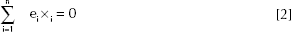
and they are obtained by solving the equations:
namely:
where s2, estimate of σ2, is,
It is known that
Calibration
The equation
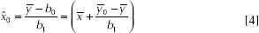
where
Note that the ratio-type estimate is biased because, in general:
However, the confidence interval for x0 may be obtained by the exact method relying on the application of Fieller's theorem (15) (see ref. 16 for details), or by resorting to the approximate variance of
where
It can be shown (17, p. 287) that the approximate confidence limits given by the delta method are, for most purposes, valid approximations to the exact confidence limits given by Fieller's theorem when
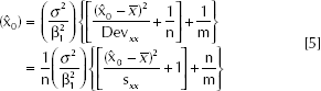
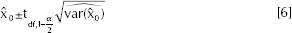
The (1-α)100% approximate confidence interval of x0 is:
where
Remark 2
The term
LAD Estimator
The LAD regression is a robust method particularly useful when error distributions are heavy tailed or asymmetrical. The LAD estimator is defined by:
Unlike OLS, there are in general no explicit expressions for LAD estimates; however, nowadays very fast algorithms to compute them are available (for example the function qr in package quantreg of R software and command call lav in proc iml of SAS software).
Regardless of the algorithm adopted, the LAD regression line must, by definition, pass through 2 data points; hence, the number of non-zero residuals is n-2.
Consider equation [1] in the special case of “regression” when explanatory variables are absent. It becomes: yj= β0+ εj. In the context of OLS regression, it is well known that b0=mean of the sample data. On the other hand, in LAD regression, owing to the minimization criterion [7], it results that b0=median of the sample data.
Let ν be the median of the random variable Y with probability density function f(Y) and
When the distribution is symmetrical, the mean and median coincide.
For Y normally distributed with location parameter ν and standard deviation σ:
When Y is normal, the ratio
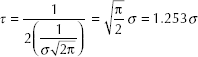
The parameter τ is estimated according to McKean and Shrader (19) as used by call lav in proc iml of SAS software.
The LAD regression is to the OLS regression what the sample median is to the sample mean. For instance, both the sample mean and the OLS estimators are determined and influenced by the whole set of observations, whereas the sample median and the LAD regression estimates are determined by only a subset of observations.
The estimated covariance matrix of
Coherently, the analogue of equation [4] is obtained by substituting
M and MM estimators
In the M-estimation the vector
However, in order to be scale equivariant, the M-estimator must satisfy:

where s is now a robust scale estimate.
By setting the partial derivatives of ρ to 0, the M-estimator is obtained by solving the equations:
These equations, unlike those in [2], are nonlinear equations in the constants and they may be solved by resorting to an iterative reweighted least squares (IRLS). Let's define the weight function
Provided that initial robust estimates s0 of the scale factor and
Define the scaled residuals
Compute the updated estimate
Iterate 1) and 2) until convergence.
Among the several ρ functions proposed in literature, we considered the popular bisquare weight (also called biweight) function (9). The corresponding ψ function is,
The estimated covariance matrix of
where
Moreover, asymptotically
It is worth noticing that Yohai (23) shows that an MM estimator is obtained when the initial estimates s0 and
The analogue of equation [4], i.e.
It can be shown that, under some regularity conditions (24) on f(y) and ψ:
With regards to
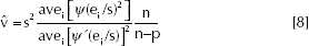
In Remark 2 the meaning of the two components of expression [5] was underlined; in the OLS approach their estimates are based on the unbiased efficient estimate of σ2 given by [3]. In the M-estimation setting, Fisher and Horn (7, pp. 132-133) suggested to use
Moreover, to estimate the variance of ε, the authors suggested to use:
where the summation is over those
Consequently
To compute the approximate confidence interval of x0 the expression [6] is used, after substituting
Coverage Assessment
Confidence intervals are computed. The confidence level 1-α=0.9 is used. The estimated coverage probability is the proportion of M confidence intervals including the true “concentration value”, defined as calibration point in “the Monte Carlo scheme” subsection. A possible criterion to consider an estimated coverage acceptable is that it should fall inside the interval
Results
First, we observed that in our study the highest value for the threshold of the criterion g mentioned in the “calibration” subsection is 0.03 (in the scenario with σ=0.7, contamination percentage 20, contamination intensity c=8, contamination modality a). This justifies the use of the approximate delta method to compute the confidence interval for x0.
Secondly, it is worth noting that the regression parameter coverages are all acceptable and included in the interval (88.48-91.52) (data not shown).
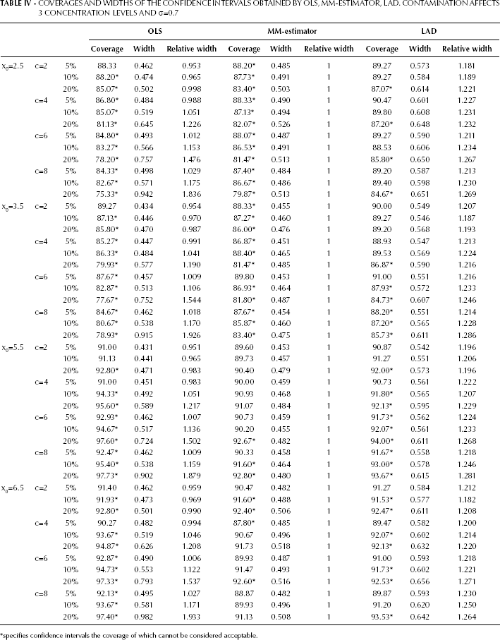
Four tables report the results of the study in terms of coverage and width of the confidence intervals obtained by OLS, LAD, and MM-estimator. Tables I and II report the results from the contamination of all concentration levels, with σ=0.2 in Tab. I and σ=0.7 in Table II. Tables III and IV report the results from the contamination occurring only at the three lowest concentration levels, with σ=0.2 in Tab. III and σ=0.7 in Table IV. Asterisks specify confidence intervals, the coverage of which cannot be considered acceptable according to the criterion for coverage assessment adopted (see “Coverage assessment” subsection).
We will first consider Tab. I and in particular the scenario where x0=2.5, which is the most critical from a technical point of view. As expected, in the absence of contamination the coverage of OLS estimator interval is at the nominal level and its width is the smallest among those of the procedures considered; however, OLS performance deteriorates in the presence of contamination. In fact, although the width tends to increase when contamination increases, the coverage tends to decrease and to appear unacceptable. With regard to the robust methods, when contamination is absent the MM-estimator performance is similar to OLS in terms of both coverage and width, whereas the LAD interval has an acceptable coverage at the expenses of a high width (1.25 times the OLS one, as expected). Therefore, in the presence of contamination we can observe a trade-off between width and coverage. The MM estimator seems resistant to contamination, as the intervals widths remain short, but this is associated with a reduction in coverages. On the contrary, LAD intervals widths are constantly larger than those of the MM-estimator so that their coverages are acceptable at the nominal level, i.e. coverage acceptability is paid in terms of imprecision.
COVERAGES AND WIDTHS OF THE CONFIDENCE INTERVALS OBTAINED BY OLS, MM-ESTIMATOR, LAD. CONTAMINATION AFFECTS ALL CONCENTRATION LEVELS AND σ=0.2
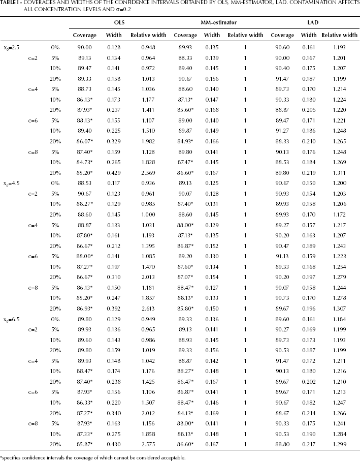
specifies confidence intervals the coverage of which cannot be considered acceptable.
Similar considerations apply to the remaining calibration points (x0=4.5, x0=6.5) and to the findings reported in Table II.
COVERAGES AND WIDTHS OF THE CONFIDENCE INTERVALS OBTAINED BY OLS, MM-ESTIMATOR, LAD. CONTAMINATION AFFECTS ALL CONCENTRATION LEVELS AND σ=0.7
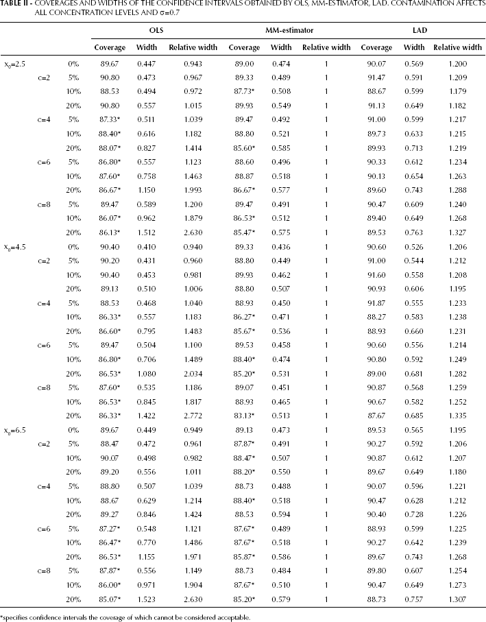
specifies confidence intervals the coverage of which cannot be considered acceptable.
With reference to Tab. III, it is important to note that x0=2.5 and x0=3.5 explore a situation where the unknown samples are expected to be contaminated, while x0=5.5 and x0=6.5 explore a situation where the unknown samples are expected to be uncontaminated, coherently with remark 1. As far as x0=2.5 and x0=3.5 are concerned, it is easy to notice that the findings are similar to those in Table I. The attention now focuses on x0=5.5 and x0=6.5. The unknown sample is uncontaminated; on the other hand, the variance of its response location measures (
COVERAGES AND WIDTHS OF THE CONFIDENCE INTERVALS OBTAINED BY OLS, MM-ESTIMATOR, LAD. CONTAMINATION AFFECTS 3 CONCENTRATION LEVELS AND σ=0.2
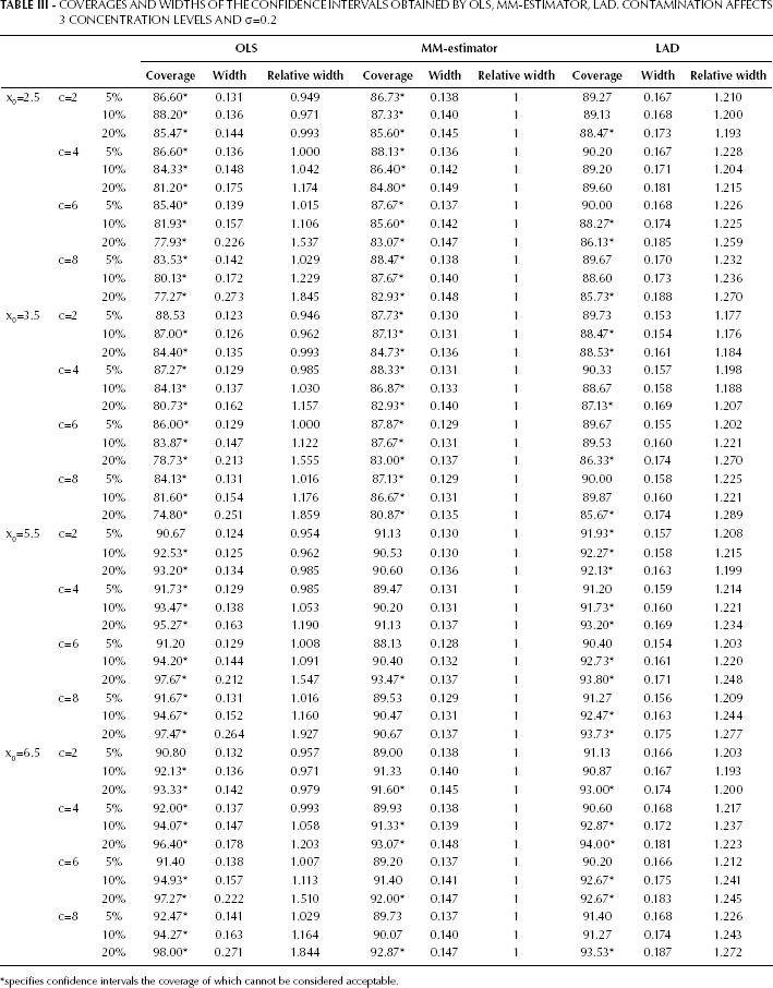
specifies confidence intervals the coverage of which cannot be considered acceptable.
Similar considerations apply to the scenarios reported in Table IV.
COVERAGES AND WIDTHS OF THE CONFIDENCE INTERVALS OBTAINED BY OLS, MM-ESTIMATOR, LAD. CONTAMINATION AFFECTS 3 CONCENTRATION LEVELS AND σ=0.7
specifies confidence intervals the coverage of which cannot be considered acceptable.
Discussion
In real-time PCR calibration, it seems reasonable to postulate a heterogeneous distribution of measurements errors; hence, robust regression methods should be implemented to estimate x0 and to compute its confidence interval. However, to select the most appropriate robust procedure a thorough investigation of the features of the process generating measurements in each laboratory is needed.
As pointed out by one of the anonymous reviewers, in recent years different methods for quantification have been developed as an alternative to the Ct method used under the condition of constant efficiency. On the other hand we are aware that the Ct method is still used in several laboratories and our results could thus be helpful for these cases.