Sage Journals: Discover world-class research

Abstract

The diffusion-weighted-dependent attenuation of the MRI signal E(b) is extremely sensitive to microstructural features. The aim of this study was to determine which mathematical model of the E(b) signal most accurately describes it in the brain. The models compared were the monoexponential model, the stretched exponential model, the truncated cumulant expansion (TCE) model, the biexponential model, and the triexponential model. Acquisition was performed with nine b-values up to 2500 s/mm² in 12 healthy volunteers. The goodness-of-fit was studied with F-tests and with the Akaike information criterion. Tissue contrasts were differentiated with a multiple comparison corrected nonparametric analysis of variance. F-test showed that the TCE model was better than the biexponential model in gray and white matter. Corrected Akaike information criterion showed that the TCE model has the best accuracy and produced the most reliable contrasts in white matter among all models studied. In conclusion, the TCE model was found to be the best model to infer the microstructural properties of brain tissue.

Keywords

diffusion MRI model accuracy kurtosis cumulant expansion Akaike information criterion brain IVIM

Introduction

Diffusion MRI (dMRI) is a powerful in vivo method for exploring biological microstructures.¹ The contrast of diffusion-weighted (DW) images is dependent on the magnitude of the diffusion-weighting factor (b-value). In clinical practice, especially for fast and early detection of ischemic stroke, DW images are generally acquired with a unique b-value (b = 1000 s/mm²). The geometric mean of DW images over three spatial directions is then used to calculate apparent diffusion coefficient (ADC) maps² with the help of a monoexponential model (MEM) formalism. As it uses the same limited range of b-values but is acquired for 6–60 spatial directions,³ diffusion tensor imaging is also an MEM that includes the effect of water diffusion anisotropy³ and leads to the calculation of a rotationally invariant form of the ADC, the mean diffusivity.

On the other hand, the higher the b-value, the more sensitive the DW images are to smaller absolute random displacements of water molecules, and therefore to the microscopic structures of brain tissue.¹ Therefore, high b-value dMRI consists of recording series of DW images with successively increasing b-values up to relatively high values (b ~2500 to ~12,000 s/mm²). The number of spatial direction measures acquired is adapted depending on the time constraints. The DW-dependent attenuation of the MRI signal obtained in each image pixel is related by Fourier transformation to the water displacement probability distribution (q-space method). In brain tissue, the standard deviation of this distribution has a characteristic length scale of tenths of μm,^4,5 making it possible to investigate some microstructural changes related to cerebral insults.⁵ However, Fourier transformation of the DW-dependent attenuation of the MRI signal (q-space) requires experimentally challenging conditions, whereas signal modeling is more flexible. Indeed, the DW-dependent attenuation of the MRI signal (designed as E(b)) acquired with intermediate or high b-values needs to be modeled numerically with a mathematical function describing its non-exponential decay, which is relevant to the postulated properties of the microscopic structures present in brain tissues.^4,6–8 High b-value dMRI modeling and q-space are very sensitive to microscopic water displacements, highlighting white matter (WM) structures^7,8 or cerebral insults in animals^9–12 and in human brains,^5,13 and thus having a potential clinical interest.

Two types of models are needed for the study of diffusion imaging. The first (signal models) describes empirically how the E(b) signal decays, whereas the second (tissue models) describes how the signal relates to the underlying tissue microstructure. However, for the former, several signal models have been developed to perform high b-value dMRI modeling, ie, to fit the E(b) signal^4,6–8: the biexponential model (BEM),^7,14–18 the triexponential model (TEM),^3,7,12 the stretched exponential model (SEM),^19–23 and the truncated cumulant expansion (TCE) model.^1,24–26 The latter is closely related to the diffusional kurtosis imaging model.^1,24–26 However, to date, no studies have compared the contrast and goodness-of-fit of all of these four different models on the same scans and the best model to be used in research imaging protocols remains a matter of debate. The aim of this study was to determine which mathematical model is the best to analyze the DW-dependent attenuation of the MRI signal of the human brain in a range of clinically accessible b-values, in terms of accuracy, contrast, and insensitivity to artifacts. Accuracy was studied with the Akaike information criterion (AIC), which is a reference statistical index of goodness-of-fit that makes it possible to test simultaneously the accuracy of different models potentially differing by their degrees-of-freedom.

Methods

Acquisition design

Subjects and patients

For the purpose of this study, we included 12 healthy human control subjects without memory dysfunction. The study protocol (ClinicalTrials.gov Identifier: NCT01686516) complied with the principles of the Declaration of Helsinki and was approved by the local ethics committee (South West France and Overseas French Departments I–II, France). Five subjects were young (26 ± 4 years) and seven were old (66 ± 6 years). To illustrate the clinical interest and the feasibility of high b-value dMRI acquisitions in hospital emergencies, a patient was scanned 4 days after a serious stroke infarct with a protocol identical to those employed for healthy subjects. Written informed consent was obtained from every subject/patient before participation.

MRI acquisitions

Magnetic resonance images were acquired with a Philips Achieva® 3 T magnet (maximum magnetic field gradient intensity: 40 mT/m) equipped with an eight-channel coil. DW spin echo images (31 slices covering the entire brain) were acquired with a pulsed gradient spin echo dMRI pulse sequence (A/8 = 34.5/25 ms, constant diffusion time t_d = 27 ms) with an echo-planar (EP) imaging readout (TR/TE = 4212/70 ms). DW images were recorded with an increasing range of b -values (0, 100, 200, 500, 750, 1000, 1500, 2000, and 2500 s/mm², N_b = 9) obtained by increasing the intensity of the magnetic field gradients. For each b -value, the scanner provided the geometric mean of DW images acquired in the read (R), phase (P), and slice (S) encoding directions. Spatial resolution used was 2 mm × 2 mm (matrix size 128 × 128) and slice thickness was 4 mm. Reconstruction for parallel imaging with sensitivity encoding for fast MRI (SENSE) was used with a SENSE factor of 2. Total dMRI scan duration was seven minutes, a duration compatible with the use of our protocol in hospital emergencies.

Image processing

Image registration

Otsu's method of histogram analysis²⁷ was used to extract the brain image from skull and background noise. To limit the effect of the patient's head motion²⁸ and susceptibility-related geometrical distortions of EP images,²⁸ Matlab® methods applying, respectively, soft linear registration and soft local, nonlinear registration of EP images were used.^29–31 DW images were also visually checked for other remaining artifacts. Pixel-by-pixel division of registered DW images S(b) by S₀ image (image acquired with no diffusion weighting) was performed to obtain images of the normalized DW-dependent attenuation of the MRI signal E(b) = S(b)/S₀.

Segmentation and regions-of-interest (ROIs)

Segmentation accuracies of the packages FreeSurfer, SPM, and FSL have been previously compared, and for WM, a higher volumetric segmentation accuracy was found with the FSL package.³² In this study, higher significance was given to WM compared to gray matter (GM). WM is less prone to partial volume effects of cerebrospinal fluid (CSF), so it is more reliable for unbiased diffusion model accuracy comparisons. EP images can be segmented, but care must be taken when doing so.³³ Segmentation of EP images was done with the FSL segmentation algorithm FAST (FMRIB's automatic segmentation tool), which provided binary masks that served as ROIs corresponding to CSF, GM, and WM.

Models of the E(b) signal

The parameter S₀ was not considered as a free parameter in any of the models. To fit pixel-by-pixel the S(b)/S₀ images, the following models were used:

Monoexponential model

This model of the E(b) signal approximates water diffusion in the tissue as Gaussian. It also has the following form for diffusion approximated as isotropic^14,15:

E (b) = S (b) / S_{0} = exp (- b \cdot A D C)

(1)

where ADC is the previously defined apparent diffusion coefficient. The MEM is generally used for a low b-value range (300–1500 s/mm²), where the Gaussian diffusion approximation is valid.^14,15 For the intermediate b-value range used here, deviations of the E(b) signal from an MEM are known,⁴ but MEM was used in this work as a reference model for comparison of accuracies. The MEM has only one degree-of-freedom (N_dof = 1).

Stretched exponential model

The SEM has the following form^19–23:

E (b) = [- {(b \cdot D D C)}^{a}]

(2)

where DDC is the distributed diffusion coefficient, ie, it is the abscissa relative to the peak of a distribution of diffusion coefficients, hypothesized in the SEM to exist in the tissue.^19–23 In brain, DDC exhibits lower values than ADC does.^20–23 A weak anomalous exponent α indicates a strongly non-exponential E(b) signal, equivalent in the SEM hypothesis to a broad distribution of diffusion coefficients.^19–23 The SEM is a low-degree-of-freedom model (N_dof = 2).

Truncated cumulant expansion

The second-order TCE of the signal E(b) is a mathematical model closely related to the q-space method,^24,25 but it does not use Fourier transformation as it has the following analytical formulation^1,24–26:

E (b) = \exp [- b \cdot D_{a p p} + (b^{2} \cdot D_{a p p}^{2} \cdot K_{a p p}) / 6]

(3)

where D_app is the cumulative ADC and K_app is the apparent kurtosis. The second-order TCE has a low degree-of-freedom (N_dof = 2). The diffusional kurtosis imaging model is a tensorial form of the second-order TCE model acquired in clinically feasible conditions, ie, with two non-null b-values and at least 15 directions.^24,25

In brain, D_app exhibits higher values than ADC does.^24–26 Apparent kurtosis K_app is commonly interpreted as: (i) representative of the presence of restricted diffusion^4,24 or (ii) representative of the presence of tissue microscopic heterogeneity.^1,25 Indeed, in the latter case, it is possible to calculate the standard deviation of the local diffusivities (σ) in the following manner^1,25:

σ = \sqrt{(K_{app} \cdot D_{app}^{2}) / 3}

(4)

The parameter σ represents the dispersion of the correlation function of the disorder existing in the biological medium, ie, σ is a parameter estimating the structural disorder frequency of barriers encountered during the diffusion of water molecules in the tissue, like those created by the spatial distribution of biomembranes.¹

Biexponential model

The BEM has the following form^15–18:

E (b) = F_{fast} \cdot exp (- b \cdot D_{fast}) + F_{slow} \cdot exp (- b \cdot D_{slow})

(5)

with

F_{fast} + F_{slow} = 1

This models the sum of the contribution (with no exchange) of two water pools (F_fast and F_slow), each associated, respectively, with expected “fast” and “slow” ADCs (D_fast and D_slow).^15–18 The BEM has three degrees-of-freedom (N_dof = 3).

Triexponential model

To estimate the signal attenuation properties both at low¹⁴ and high b-values,¹⁵ three exponential functions are combined^3,7,12 to express the TEM as:

E (b) = F_{1}^{*} \cdot exp (- b \cdot D_{1}^{*}) + F_{2} \cdot exp (- b \cdot D_{2}) + F_{3} \cdot exp (- b \cdot D_{3})

with

F_{1}^{*} + F_{2} + F_{3} = 1

(6)

where

F_{1}^{*}

and

D_{1}^{*}

could be related to the properties of the blood micro-circulation water fraction with intravoxel incoherent motions (IVIM)¹⁴, CSF water fraction,^3,14 or a mix of both.¹⁴ As it is representative of blood microcirculation pseudo-diffusion, D₁* could attain values of tenths of μm²/ms, which is much greater than the true diffusion coefficient of free water,¹⁴ which is 3 μm²/ms. F₂ is analogous to F_fast, F₃ is analogous to F_slow. The TEM has six degrees-of-freedom (N_dof = 6).

Numerical implementation

E(b) images were fitted pixel-by-pixel over the full b-value range (0–2500 s/mm²) with an in-house Matlab® program implementing the models presented (MEM, SEM, TCE, BEM, TEM). Regression convergence of nonlinear systems described by equations (1), (2), (3), (5), and (6) was performed by simple least square minimization of the sum of squared residuals (SSR) of the fit, using 800 iterations of the Nelder–Mead simplex algorithm (fminsearch Matlab® function).³⁴ This procedure allowed the rapid calculation of the SSR maps and parametric maps corresponding to the free parameters of the models $(A D C, D D C, α, D_{app}, D_{fast}, F_{f ast}, D_{s low}, F_{slow}, D_{1}^{*}, F_{1}^{*}, D_{2}, F_{2}, D_{3} F_{3})$ .

Statistical analysis

Analysis of model contrasts

Parametric images were visually checked for artifacts. The contrast comparison between anatomically neighboring structures (ie, CSF compared to GM, GM compared to WM) for values of spatially averaged quantitative parameters $(A D C, D D C, σ, D_{app}, σ, K_{app}, D_{fast}, F_{f ast}, D_{slow}, F_{slow}, D_{1}^{*}, F_{1}^{*}, D_{2}, D_{2}, F_{2}, F_{3})$ was tested with a Kruskal–Wallis nonparametric one-way analysis of variance with a P-value correction for multiple comparisons using the Holm–Bonferroni method. This was performed with the R statistical software³⁵ using the “kruskal” function of the “agricolae” package. Conventions used for statistical significance were the following: P < 0.001 (***), P < 0.01 (**), P < 0.05 (*).

Spearman's rank correlation implemented in Matlab® was used to obtain the coefficient of correlation R between the values of different diffusion parameters measured in the WM for the 12 subjects, together with the corresponding risk probability. The significant risk probability level chosen was P < 0.05.

Analysis of goodness-of-fit

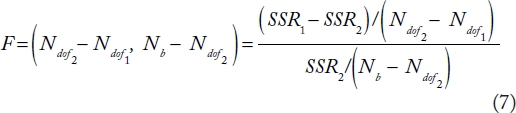
F-tests. To calculate the F-statistic associated with model comparisons,^26,36,37 the approach proposed in the work of Yoshiura et al was used,³⁶ where the F-value is defined as:

F (N_{d o f_{2}} - N_{d o f_{1}}, N_{b} - N_{d o f_{2}}) = \frac{(S S R_{1} - S S R_{2}) / (N_{d o f_{2}} - N_{d o f_{1}})}{S S R_{2} / (N_{b} - N_{d o f_{2}})}

(7)

where SSR₁ is the SSR of model 1 and SSR₂ those of model 2, each having N_dof₁ and N_dof₂ degrees-of-freedom, respectively, and where N_b is the number of b-values. Practically, F-values were obtained after spatial averaging of segmented SSR maps³⁵ in ROIs. F-values were also averaged over the population sample. F_exp (the experimental F-value) was then compared to F_theo (the theoretical F-value) at risk probability P < 0.05 in the Fisher–Snedecor table.³⁷

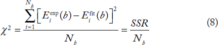
AIC. The AIC has a particularly simple form when the E(b) signal is fitted by simple least square³⁸:

A I G = N \cdot 1 n (χ^{2}) + 2 \cdot N_{d o f}

with

χ^{2} = \frac{\sum_{t = 1}^{N_{b}} {[E_{i}^{\exp} (b) - E_{i}^{fit} (b)]}^{2}}{N_{b}} = \frac{S S R}{N_{b}}

(8)

where E^exp(b) is the experimental DW-dependent attenuation of the MRI signal and E^fit(b) is the discrete model used for fitting, and where [E^exp(b) - E^fit(b)] is the residual of the fit. N represents the number of subjects and N_dof represents the degrees-of-freedom of a given model. When using limited sample sizes (when N/N_dof < 40), it is also convenient to define a corrected AIC termed AICc³⁸:

A I C c = A I C + \frac{2 N_{dof} (N_{dof} + 1)}{N - N_{dof}}

(9)

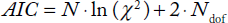
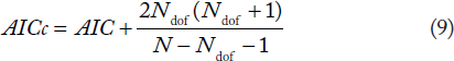
Indeed, to be able to compare efficiently the accuracy of the models, an accurate penalty for models with high degrees-of-freedom needs to be taken into account.³⁸ The lower the AICc value, the better the model describes the experimental data obtained in the population sample.³⁸

Results

Contrast analysis

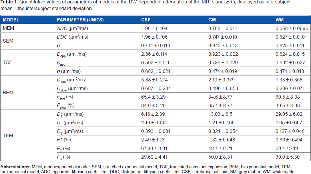
Parametric maps and corresponding contrasts are shown in Figure 1 (for MEM, SEM, and TCE) and Figure 2 (for BEM and TEM), and quantitative values are given in Table 1. The tissue contrasts between adjacent tissues are shown in the bar charts in Figures 1 and 2.

Figure 1

Parametric images (one slice) of the MEM (ADC images top) of the SEM (DDC and α maps bottom) and of the second-order TCE (D_app, K_app, and σ maps) in a representative (aged) subject Bar charts show the values of the free parameters of the models (mean ± the standard deviation in the population sample) Statistically significant tissue contrast differences for anatomically-neighboring tissues are also shown (*P<0 05 **P<0 01 ***P<0 001)

Figure 2

Parametric images (one slice) of the BEM and of the TEM in a representative (aged) subject. Bar charts show the values of the free parameters of the model (mean ± the standard deviation in the population sample). Statistically significant tissue contrast differences for anatomically-neighboring tissues are also shown (*P<0.05, **P<0.01, ***P<0.001).

Table 1

Quantitative values of parameters of models of the DW-dependent attenuation of the MRI signal E(b), displayed as intersubject mean ± the intersubject standard deviation.

MODEL	PARAMETER (UNITS)	CSF	GM	WM
MEM	ADC (<m²/ms)	1.96 ± 0.104	0.768 ± 0.011	0.658 ± 0.0096
SEM	DDC (<m²/ms)	1.96 ± 0.106	0.747 ± 0.010	0.627 ± 0.010
SEM	α	0.744 ± 0.018	0.842 ± 0.013	0.825 ± 0.011
TCE	D_app (<m²/ms)	2.36 ± 0.114	0.923 ± 0.022	0.824 ± 0.015
	K _app	0.592 ± 0.016	0.789 ± 0.029	0.992 ± 0.027
	σ (<m²/ms)	0.682 ± 0.021	0.474 ± 0.019	0.474 ± 0.013
BEM	D_fast (<m²/ms)	3.88 ± 0.274	2.19 ± 0.379	1.33 ± 0.368
	D_slow (<m²/ms)	0.687 ± 0.284	0.490 ± 0.058	0.206 ± 0.071
	F_fast (%)	65.4 ± 3.29	34.6 ± 8.77	60.5 ± 8.38
	F_slow (%)	34.6 ± 3.29	65.4 ± 8.77	39.5 ± 8.38
TEM	$D_{1}^{*} (μ m^{2} / m s)$	6.16 ± 2.39	13.03 ± 8.5	29.05 ± 6.02
	D₂ (<m²/ms)	2.16 ± 0.144	1.21 ± 0.106	1.05 ± 0.067
	D₃ (<m²/ms)	0.393 ± 0.031	0.321 ± 0.054	0.127 ± 0.048
	$F_{1}^{*} (%)$	2.49 ± 1.13	1.32 ± 0.648	0.66 ± 0.494
	F₂ (%)	67.90 ± 3.81	48.7 ± 8.21	69.4 ± 5.19
	F₃ (%)	29.62 ± 4.41	50.0 ± 8.31	30.0 ± 5.30

Abbreviations: MEM, monoexponential model; SEM, stretched exponential model; TCE, truncated cumulant expansion; BEM, biexponential model; TEM, triexponential model; ADC, apparent diffusion coefficient; DDC, distributed diffusion coefficient; CSF, cerebrospinal fluid; GM, grey matter; WM, white matter.

Artifacts and reproducibility

High sensitivity to CSF pulsatile motion artifacts was often observed in the SEM, BEM, and TEM parametric images (see Figs. 1 and 2, artifacts a round the ventricles in α, F_fast, F_slow, D_fast, D_slow, F₂ maps). $D_{1}^{*}$ in CSF, GM, and WM and D_fast in CSF showed values higher than 3 μm²/ms (Table 1), the value for the diffusion coefficient of free water. This is known to be an effect of blood circulation random flows in microvessels (IVIM phenomenon)¹⁴ or to CSF pulsations.¹⁴ In addition, TEM parameters D₁^* and F₁^* showed a high variability and weak reproducibility, as indicated by their high standard deviation in the population sample (Fig. 2 bar charts) compared to other parameters. ADC, D_app, and K_app maps were free of artifacts, especially those related to pulsatile motions (Fig. 1). The vascular network of the brain appeared as null values in K_app maps as areas where the TCE fit was not as accurate as in the tissue (Fig. 1).

Tissue contrasts.

ADC (Fig. 1), DDC (Fig. 1), D_fast (Fig. 2), D₂ and D₃ (Fig. 2) maps showed a significant intensity decrease from CSF to WM (bar charts of Figs. 1 and 2 and Table 1).

Parametric maps modeled with the BEM and the TEM, especially water fractions F_fast, F_slow, F₁, F₂, and F₃, appeared noisy and did not exhibit any evident anatomical contrast (Fig. 2).

Maps of the parameter α (Fig. 1) showed a significant but weak contrast between GM and WM (P < 0.05). Conversely, a particularly strong and anatomically well-defined contrast (P < 0.001) appeared in K_app maps, clearly revealing the structure of the WM and the GM (Fig. 1). Areas with higher intensities on K_app maps appeared to be WM substructures, maybe areas of high tissular complexity (Fig. 1). In C maps, a strong contrast differentiating GM/WM tissues and CSF (P < 0.001) was observed (Fig. 1).

Contrast correlations

The correlation between the diffusion parameters obtained in WM was then examined. There was a strong correlation between DDC and ADC (R = 0.9580, P < 0.05), but not between DDC and D (R = 0.4964, P > 0.05) or between DDC and α(R = -0.1049, P ≫ 0.05).

However, there was a positive correlation between D_app and ADC (R = 0.6130, P< 0.05), between D_app and K_app (R = 0.6224, P < 0.05), and between D_a and σ (R = 0.9161, P < 0.05), as shown in Figure 3. The parameters extracted from BEM and TEM, especially the ADCs of the models, showed no correlation either with ADC or with D_a (P > 0.05, data not shown).

Diffusion model contrast in stroke

The E(b) signal attenuation was also modeled in a stroke patient. The classical high T2-weighted signal and the decreased intensity of the ADC maps² were observed in the lesion (Fig. 4A and 4B, respectively). There was a similar decrease in DDC and decrease in D_app in the entire lesion. In the stroke lesion infarcted WM (Fig. 4D), there was a strong increase in K_app in infarcted WM (from 0.9 to 1.81) and a decrease in σ (from 0.46 to 0.42 μm²/ms). In the GM of the lesion, σ maps showed a greater decrease (from 0.61 to 0.43 μm²/ms). For BEM in infarcted GM (Fig. 4E), there were both a strong increase in F_slow (up to 69%) and a strong decrease in D_slow (from 0.57 to 0.18 μm²/ms). F₁* maps representing the magnitude of the IVIM microcapillary perfusion were very noisy as in the healthy population sample, but the delineation of the infarcted area in F₁^* maps showed a larger extension of the lesioned area than in the ADC map (Fig. 4F, arrowhead).

Figure 3

Positive correlation between D_app values and K_app values (top), D_app values and ADC values (middle), D_app values and σ values (bottom), obtained for the 12 subjects in the white matter of the sample population. Spear man's coefficient of rank correlation (R) is also indicated for each linear regression (P < 0.05).

Figure 4

an MRI slice of multi-parametric imaging in a patient with stroke (four days after the infarct), showing both grey and white matter insults in (A) T₂-weighted images (T2W) acquired with TE/TR = 80/8624 ms; (B) maps of the MEM: ADC; (C) maps of the SEM; (D) maps of the second-order TCE model; (E) maps of the BEM; and (F) two maps of the TEM: F₁* and D₁*.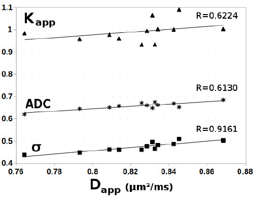

Models’ goodness-of-fit

For the sake of clarity, we present the modeled E(b) signals obtained in the WM of a representative subject (Fig. 5, left) and the corresponding SSR maps (Fig. 5, right). The SSR maps correspond to the anatomical location of the slice of the parametric maps presented in Figures 1 and 2. To be visually indicative of the compared goodness-of-fit, both the residual of the E(b) signal and the SSR maps were multiplied by N_dof, the degree-of-freedom of each model (Fig. 5). Figure 5 is also an illustration that an objective mathematical method is needed to differentiate which functions given by equations (2)–(5) are the best to describe the E(b) signal experimentally.

Figure 5

Left: the experimental diffusion-weighted-dependent attenuation of the MRI signal (the E(b) signal, empty triangles ▿) and the absolute value of the residual of the fit times the degree-of-freedom N_dof (dotted lines, black squares ▪, values multiplied by a factor 10) obtained in WM in a representative subject. Separate subfigures show the modeling by the MEM, by the SEM, by the second-order TCE model, by the BEM, and by the TEM, all represented by black dots (-•-). Right: SSR times N_dof maps of the models for an anatomical slice, which corresponds to the slice presented for the parametric images of the models in Figure 1 and Figure 2

F-tests

When analyzed with F-tests in all the segmented brain regions, the BEM, TEM, and TCE all performed better than the MEM for modeling the E(b) signal (P < 0.05). The BEM performed better than the TEM in all the brain areas (P < 0.05). The TCE was found to be a better model than the BEM in GM and WM (P < 0.05). The TCE and SEM have the same number of degrees-of-freedom (N_dof = 2), so they cannot be compared with the F-test method given in the work of Yoshiura et al, Equation (7).³⁶

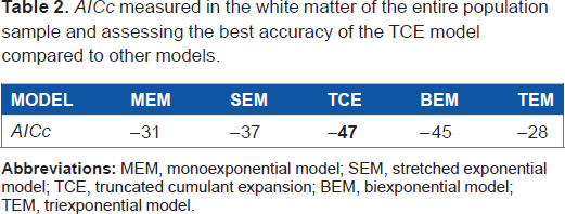
AICc

When analyzed with AICc, the accuracy of models measured in the WM were as follows: TCE > BEM > SEM > MEM > TEM (Table 2). The accuracy (weak AICc) for modeling the E(b) signal in the WM tissue with the TCE model was better than the others (Table 2).

Table 2

AICc measured in the white matter of the entire population sample and assessing the best accuracy of the TCE model compared to other models.

MODEL	MEM	SEM	TCE	BEM	TEM
AICc	-31	-37	-47	-45	-28

Abbreviations: MEM, monoexponential model; SEM, stretched exponential model; TCE, truncated cumulant expansion; BEM, biexponential model; TEM, triexponential model.

In the representative fit accuracy provided, the residual values for b_max =2500 s/m² was high for MEM, SEM, BEM, TEM but was low for the TCE model (Fig. 5), which illustrates the good convergence of this latter model for the highest b-values used in this work. However, for very low b-values (b = 100 and 200 s/mm²), a slight deviation of the TCE fit was observed (Fig. 5). Although the accuracy of the TCE model was the best in the WM, relatively high SSR values were also observed for the TCE fit in the GM area contaminated by CSF partial volume effects (Fig. 5, right).

Discussion

The main finding of the present study is that the TCE is the most appropriate mathematical function to model the DW-dependent attenuation of the MRI signal E(b) in the WM tissue. Our results showing the excellent goodness-of-fit of the TCE model in WM compared to the BEM model agree well with those in the previous study,²⁶ which used the geometric mean of DW images of five subjects, with N_b = 16 and b-factors up to 2500 s/mm² and compared only the BEM and TCE models.²⁶ The accuracy of these two models was compared using a ratio of F-values, a noise-independent method.²⁶ However, the F-test approach does not make it possible to compare more than two models simultaneously and efficiently. The additional strength of our methodology is that we estimated the models’ goodness-of-fit in a larger sample size and used a powerful statistical index (AICc). This allowed us to compare more than two models irrespective of their degree-of-freedom. We were thus able to compare the TCE model simultaneously with other models such as the SEM, BEM, and TEM. Our results showed an apparent discrepancy between the accuracies obtained with the F-test (Equation (7)) and AICc (equations (8) and (9)). Indeed, the latter method lead to a better accuracy of the MEM (N_dof = 1) compared to the TEM (N_dof = 6). This is because the Equation (9) has a term in 2N²_dof + 4N_dof whereas Equation (7) scales only in N_dof, and because a larger penalty is applied to models with a high degree-of-freedom when the AICc approach is used (Table 2).

In our work, the TCE was found to be superior not only to the BEM but also to the TEM and the SEM in terms of accuracy, contrast, and insensitivity to artifacts. The TCE provided a strong contrast between GM and WM in K_app maps, whereas α, F_fast, or F_slow and F₁, F₂, or F₃ maps gave a poorly defined anatomical tissue contrast. The poor contrast and low reproducibility of the quantitative parameters of the BEM and the TEM and the poor fit stability of the TEM⁷ may also be because of the fact that only one water pool might be present in the tissue,^1,26 contrary to the assumptions of these models. It has been noted that overfitting errors may accumulate along the b -value range, especially for TEM, which is overdetermined.⁷ It could be noted that the BEM is almost always used with CSF-suppressed dMRI sequences,^7,16,17 thus avoiding the presence of CSF water, which could be mistaken for an additional water pool. On the contrary, the low-degree-of-freedom TCE model, which has no a priori hypothesis concerning the number of water pools, has previously been shown to be robust to infer WM properties both for acquisitions with or without CSF suppression.³⁹

However, for the TCE fit, relatively high SSR values were observed in the GM area contaminated by CSF partial volume effects, as has already been reported.²⁶ The mixing between partial volume effects of CSF water and tissue water was suspected to favor a large and non-physiologic bicompartmental attenuation of the E(b) signal.²⁶

A correlation between the related parameters ADC and D_app was found in WM, and this strong linear relationship is an experimental confirmation that the TCE model adequately extends the MEM. Self correlation was also found between the TCE parameters D_app, K_app, and σ. This means that the parameters of the TCE model are self-consistent. In other words, there is a relation between quantity D (related to the cumulant of order one in b) and between quantity K_app (related to the cumulant of order two in b). DDC also correlated well with ADC, but there was no correlation between DDC and α, the two SEM parameters. Furthermore, no significant correlations were found between ADC and the diffusion coefficients of BEM and TEM.

dMRI makes it possible to obtain signals related to tissue microstructure, but it has some drawbacks. In fact, the spatial resolution of EP images is lower than those of T₁-weighted images (anatomical MRI). Consequently, segmentation of EP images is far from providing an accurate differentiation of the GM and of the subcortical WM like those obtained with the segmentation of T₁-weighted images.⁴⁰ Owing to these intrinsic limitations of EPI-related methods, our study focused only on WM, which dominates by its large volume both the volume of the GM and the volume of the subcortical WM. Apart from this point, our study has the following limitations:

First, using more directions of diffusion measures might potentially refine the comparisons of accuracies. Nevertheless, considering that the microstructures present in tissue are of unknown nature, different tensorial forms of equations (2),²³ (5),⁴¹ and (6)³ with different degrees-of-freedom exist. On the other hand, for a given model, the degrees-of-freedom must be unequivocally defined in Equations (8) and (9). This further complicates the comparisons of models but will be addressed in a future study. Consequently, at present, we are using acquisition conditions very close to those in the study of Kiselev and Il'yasov,²⁶ where unidirectional fitting of the geometric average of DW images was used. This could potentially limit the study of WM, which has a non-null degree of anisotropy,²⁶ but a simple modeling design has the advantage of defining unequivocally the degrees-of-freedom of the models compared, a condition required for efficient accuracy comparisons.

Secondly, our conclusions about the accuracy of the models might be in part limited because model's accuracies were measured in a defined experimental context determined by the maximum b-value used (b_max = 2500 s/mm²). However, this b-value range is considered to be suitable for medical imaging in routine protocols^24–26 and the aim of our study was to determine the best model of the E(b) signal in such conditions. The use of b-values higher than 2500 s/mm² has the potential to better resolve the microstructural features of tissue but also has the disadvantage to decrease the signal-to-noise ratio. Some studies suggested that SEM^20,22 or BEM^13,16,17 are efficient models only when the b-value range is sufficiently high, and supposedly less effective for an intermediate b-value range. However, the precise b-value range where these models were considered as accurate was not explicitly nor consensually defined, as it was found to varies between studies (for SEM^19–23 and for BEM^15–18) and was not systematically compared to the theoretical b-value limit of modelling accuracy given by the radius of convergence²⁶ of their mathematical formulations. On the other hand, using the TCE model for a well-defined b-value range (0–2500 s/mm²) is consistent with its theoretical limit of accuracy.²⁶ Then, it is arguable that an adequate and flexible model that can accurately fit the E(b) signal over a high b-value range can also fit it accurately over an intermediate b-value range. This is at least the case for the more general cumulant expansion, which is adequate over an intermediate b-value range and can be extended to higher orders to describe the signal for higher b-values.⁴²

In addition, using data acquired with high b-values raises the important problem of noise, which is known to have a detrimental effect on model comparisons.⁴³ Indeed, the higher the b-value, the weaker the signal-to-noise ratio and also the higher the risk that the positive noise level is fitted by overdetermined mathematical functions.⁴² In parallel imaging, the noise in DW images is strictly positive definite⁴³ and is known to follow a Rician distribution for SENSE acquisitions.⁴³ In addition, non-homogeneity of the variance of noise occurs locally in dMRI data acquired with SENSE owing to the reconstruction process. Model accuracy comparisons in the high b-value range, especially when using high-degree-of-freedom models, may benefit from appropriate local denoising.⁴⁴ Combined model accuracy comparisons and denoising method comparisons will be used to model dMRI images acquired at high b-values and high directional resolution in subsequent work.

Conclusion

In summary, this work confirms that the low-degree-of-freedom TCE model is superior to the BEM for modeling and analyzing accurately the DW-dependent attenuation of the MRI signal E(b) in the brain tissue. Additionally, the TCE model was also found to be superior not only to the BEM but also to the SEM and the TEM, at least in WM. This reinforces the hypothesis that the phenomenological TCE model is sensitive to accurate microscopic properties of tissues, whereas the SEM, BEM, and TEM are not.^1,4,18,26 The parameter σ deducted from the TCE acquisition, an indicator of tissue microscopic heterogeneity, might prove particularly interesting as a new biomarker of microstructural changes occurring in stroke, as it would signal a change in biomembrane disorder.¹

Author Contributions

Conceived and designed the experiments: RN and BH. Analyzed the data: RN. Wrote the first draft of the manuscript: RN. Contributed to the writing of the manuscript: IS. Agreed on manuscript results and conclusions: RN, IS, and BH. Jointly developed the structure and arguments for the paper: RN, IS, and BH. Made critical revisions and approved the final version: RN, IS, and BH. All the authors reviewed and approved the final manuscript.

Footnotes

Acknowledgements

We thank F. Aubry, P. Celsis, and J. Pariente for their role in improving this manuscript.

References

Novikov

D.S.

, Kiselev

V.G.

Effective medium theory of a diffusion-weighted signal. NMR Biomed. 2010; 23(7): 682–697.

Muir

K.W.

, Buchan

, Von Kummer

, Rother

, Baron

J-C.

Imaging of acute stroke. Lancet Neurol. 2006; 5(9): 755–768.

Basser

P.J.

, Jones

D.K.

Diffusion-tensor MRI: theory, experimental design and data analysis—a technical review. NMR Biomed. 2002; 15(7-8): 456–467.

Grebenkov

D.S.

Use, misuse, and abuse of apparent diffusion coefficients. Concepts Magn Reson Part A. 2010; 36A(1): 24–25.

Hori

, Motosugi

, Fatima

Comparison of mean displacement values using high b-value q-space diffusion-weighted MRI with conventional apparent diffusion coefficients in patients with stroke. Acad Radiol. 2011; 18(7): 837–841.

Chabert

, Scifo

Diffusion signal in magnetic resonance imaging: origin and interpretation in neurosciences. Biol Res. 2007; 40(4): 385–400.

Mulkern

R.V.

, Haker

S.J.

, Maier

S.E.

On high b diffusion imaging in the human brain: ruminations and experimental insights. Magn Reson Imaging. 2009; 27(8): 1151–1162.

De Santis

, Gabrielli

, Palomba

, Maraviglia

, Capuani

Non-Gaussian diffusion imaging: a brief practical rewiew. Magn Reson Imaging. 2011; 29(10): 1410–1416.

Grinberg

, Farrher

, Ciobanu

, Geffroy

, Le Bihan

, Shah

N.J.

Non-Gaussian diffusion imaging for enhanced contrast of brain tissue affected by ischaemic stroke. PLoS One. 2014; 9(2): e89225.

10.

Grinberg

, Ciobanu

, Farrher

, Shah

N.J.

Diffusion kurtosis imaging and log-normal distribution function imaging enhance the visualisation of lesions in animal stroke models. NMR Biomed. 2012; 25(11): 1295–1304.

11.

Niendorf

, Dijkhuizen

R M.

, Norris

D.G.

, Van Lookeren Campagne

, Nicolay

Biexponential diffusion attenuation in various states of brain tissue: implication for diffusion-weighted imaging. Magn Reson Med. 1996; 36(6): 847–857.

12.

Pfeuffer

, Provencher

S.W.

, Gruetter

Water diffusion in rat brain in vivo as detected at very large b values is multicompartmental. Magn Reson Mater Phys Biol Med. 1999; 8(2): 98–108.

13.

Brugières

, Thomas

, Maraval

Water diffusion compartmentation at high b values in ischaemic human brain. Am J Neuroradiol. 2004; 25(5): 692–698.

14.

Le Bihan

, Breton

, Lallemand

, Aubin

M.L.

, Vignaud

, Laval-Jeantet

Separation of diffusion and perfusion in intravoxel incoherent motion MR imaging. Radiology. 1988; 168(2): 497–505.

15.

Clark

C.A.

, Le Bihan

Water diffusion compartmentation and anisotropy at high b-value in the human brain. Magn Reson Med. 2000; 44(6): 852–859.

16.

Maier

S.E.

, Mulkern

R.V.

Biexponential analysis of diffusion-related signal decay in normal human cortical and deep grey matter. Magn Reson Imaging. 2008; 26(7): 897–904.

17.

Mulkern

R.V.

, Zengingonul

H.P.

, Robertson

R.L.

Multi-component apparent diffusion coefficient in human brain: relationship to spin-lattice relaxation. Magn Reson Med. 2000; 44(2): 292–300.

18.

Schwarcz

, Bogner

, Meric

The existence of biexponential signal decay in magnetic resonance diffusion-weighted imaging appears to be independent of compartmentalization. Magn Reson Med. 2004; 51(2): 278–285.

19.

Zhou

X.J.

, Gao

, Abdullah

, Magin

R.L.

Studies of anomalous diffusion in the human brain using fractional order calculus. Magn Reson Med. 2010; 63(3): 562–569.

20.

Bennett

K.M.

, Schmainda

, Bennett

, Rowe

, Hanbing

, Hyde

Characterization of continuously distributed cortical water diffusion rates with a stretched-exponential model. Magn Reson Med. 2003; 50(4): 727–734.

21.

Bennet

K.M.

, Hyde

J.S.

, Schmaida

K.M.

Water diffusion heterogeneity in the human brain is insensitive to the orientation of applied magnetic field gradients. Magn Reson Med. 2006; 56(2): 235–239.

22.

Hall

M.G.

, Barrick

T.R.

From diffusion-weighted MRI to anomalous diffusion imaging. Magn Reson Med. 2008; 59(3): 447–455.

23.

Hall

M.G.

, Barrick

T.R.

Two-step anomalous diffusion tensor imaging. NMR Biomed. 2011; 25(2): 286–294.

24.

Jensen

J.H.

, Helpern

J.A.

MRI quantification of non-Gaussian water diffusion by kurtosis analysis. NMR Biomed. 2010; 23(7): 698–710.

25.

Jensen

J.H.

, Helpern

J.A.

, Ramani

, Lu

, Kaczynski

Diffusional kurtosis imaging: the quantification of non-Gaussian water diffusion by means of magnetic resonance imaging. Magn Reson Med. 2005; 53(6): 1432–1440.

26.

Kiselev

V.G.

, Il'yasov

K.A.

Is the “biexponential diffusion” biexponential?

Magn Reson Med. 2007; 57(3): 464–469.

27.

Otsu

A threshold selection method from gray-level histograms. IEEE Trans Syst Man Cyber. 1979; 9(1): 62–66.

28.

Le Bihan

, Poupon

, Amadon

, Lethimonnier

Artefacts and pitfalls in diffusion MRI. J Magn Reson Imaging. 2006; 24(3): 478–488.

29.

Periaswamy

, Hany

Elastic registration in the presence of intensity variations. IEEE Trans Med Imaging. 2003; 22(7): 865–874.

30.

Kostelec

P.J.

, Periaswamy

Image registration for MRI. Mod Sign Proc. 2003; 46: 161–183.

31.

Periaswamy

, Hany

Medical image registration with partial data. Med Image Anal. 2006; 10: 452–464.

32.

Klauschen

, Goldman

, Barra

, Meyer-Lindenberg

, Lundervold

Evaluation of automated brain MR image segmentation and volumetry methods. Hum Brain Mapp. 2009; 30(4): 1310–1327.

33.

Hadjiprocopis

, Rashid

, Tofts

P.S.

Unbiased segmentation of diffusion-weighted magnetic resonance images of the brain using iterative clustering. Magn Reson Imaging. 2005; 23(8): 877–885.

34.

Lagarias

J.C.

, Reeds

J.A.

, Wright

M.H.

, Wright

P.E.

Convergence properties of the Nelder-Mead simplex method in low dimensions. SIAM J Optim. 1998; 9(1): 112–147.

35.

R Development Core Team. R: a language and environment for statistical computing. R Foundation for Statistical Computing; Vienna, Austria: 2008. http://www.R-project.org

36.

Yoshiura

, Wu

, Zaheer

, Reese

T.G.

, Sorensen

A.G.

Highly diffusion-sensitized MRI of brain: dissociation of gray and white matter. Magn Reson Med. 2001; 45(5): 734–740.

37.

Bevington

P.R.

Data reduction and error analysis for the physical science. McGraw-Hill, Inc; NY; 1969.

38.

Turkheimer

E.F.

, Hinz

, Cunningham

V.J.

On the undecidability among kinetic models: from model selection to model averaging. J Cereb Blood Flow Metab. 2003; 23(4): 490–498.

39.

Yang

A.W.

, Jensen

J.H.

, Hu

C.C.

, Tabesh

, Falangola

M.F.

, Helpern

J.A.

Effect of cerebral spinal fluid suppression for diffusional kurtosis imaging. J Magn Reson Imaging. 2012; 37(2): 365–371.

40.

Mohammadi

, Tabelow

, Ruthotto

, Feiweier

, Polzehl

, Weiskopf

High-resolution diffusion kurtosis imaging at 3T enabled by advanced postprocessing. Front Neurosci. 2014; 8(427): 1–14.

41.

Maier

S.E.

, Vajapeyam

, Mamata

, Westin

C.F.

, Jolesz

F.A.

, Mulkern

R.V.

Biexponential diffusion tensor analysis of human brain diffusion data. Magn Reson Med. 2004; 51(2): 321–330.

42.

Özarslan

, Mareci

T.H.

Generalized diffusion tensor imaging and analytical relationships between diffusion tensor imaging and high angular resolution diffusion imaging. Magn Reson Med. 2003; 50: 955–965.

43.

Aja-Fernández

, Vegas-Sánchez-Ferrero

, Tristán-Vega

Noise estimation in parallel MRI: GRAPPA and SENSE. Magn Reson Imaging. 2014; 32: 281–290.

44.

Manjon

J.V.

, Coupé

, Concha

, Buades

, Collins

D.L.

, Robles

Diffusion weighted image denoising using overcomplete local PCA. PLoS One. 2013; 8(9): e73021.

Accuracies and Contrasts of Models of the Diffusion-weighted-dependent Attenuation of the Mri Signal at Intermediate B -values

Abstract

Keywords

Introduction

Methods

Acquisition design

Subjects and patients

MRI acquisitions

Image processing

Image registration

Segmentation and regions-of-interest (ROIs)

Models of the E(b) signal

Monoexponential model

Stretched exponential model

Truncated cumulant expansion

Biexponential model

Triexponential model

Numerical implementation

Statistical analysis

Analysis of model contrasts

Analysis of goodness-of-fit

Results

Contrast analysis

Artifacts and reproducibility

Tissue contrasts.

Contrast correlations

Diffusion model contrast in stroke

Models’ goodness-of-fit

F-tests

AICc

Discussion

Conclusion

Author Contributions

Footnotes

Acknowledgements

References