Understanding the Morphological Mismatch between Magnetic Susceptibility Source and T2 * Image

Abstract

Background and Purpose

Recent research has shown that a T2^* image (either magnitude or phase) is not identical to the internal spatial distribution of a magnetic susceptibility (χ) source. In this paper, we examine the reasons behind these differences by looking into the insights of T2^*-weighted magnetic resonance imaging (T2^*MRI) and provide numerical characterizations of the source/image mismatches by numerical simulations.

Methods

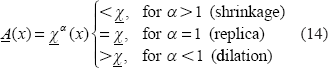
For numerical simulations of T2^*MRI, we predefine a 3D χ source and calculate the complex-valued T2^* image by intravoxel dephasing in presence and absence of diffusion. We propose an empirical α-power model to describe the overall source/image transformation. For a Gaussian-shaped χ source, we numerically characterize the source/image morphological mismatch in terms of spatial correlation and FWHM (full width at half maximum).

Results

In theory, we show that the χ-induced fieldmap is morphologically different from the χ source due to dipole effect, and the T2^* magnitude image is related to the fieldmap by a quadratic transformation in the small phase angle regime, which imposes an additional morphological change. The numerical simulations with a Gaussian-shaped χ source show that a T2^* magnitude image may suffer an overall source/image morphological shrinkage of 20% to 25% and that the T2^* phase image is almost identical to the fieldmap thus maintaining a morphological mismatch from the χ source due to dipole effect.

Conclusion

The morphological mismatch between a bulk χ source and its T2^* image is caused by the 3D convolution during tissue magnetization (dipole effect), the nonlinearity of the T2^* magnitude and phase calculation, and the spin diffusion effect. In the small phase angle regime, the T2^* magnitude exhibits an overall morphological shrinkage, and the T2^* phase image suffers a dipole effect but maintains the χ-induced fieldmap morphology.

Background

The physical principle of T2^*-weighted magnetic resonance imaging (T2^*MRI) is based on proton spin precession dephasing in an inhomogeneous fieldmap. For brain functional imaging, a brain activity contributes to the inhomogeneous fieldmap via cerebral vascular blood magnetism perturbation, which has been described by a blood oxygenation level dependent (BOLD) mechanism.^1,2 The T2^*MRI-based functional magnetic resonance imaging (fMRI) is a well-developed BOLD fMRI model, which consists of the origin of neuronal activity, the physiological expression of neurovascular coupling, the magnetic inhomogeneous fieldmap establishment of blood (tissue) magnetization, and the multivoxel T2^* image formation by intravoxel dephasing. ³ In practice, through the use of a complex echo planar imaging (EPI) sequence, a T2^*MRI study produces a complex-valued T2^* image consisting of a pair of magnitude and phase images. Conventionally, a T2^* image refers to a T2^* magnitude image because the T2^* phase counterpart remains largely unused (the exploration and exploitation of T2^* phase images are currently under pursue).^3–8 In this paper, we refer to T2^* image as a complex-valued T2^*-effect magnetic resonance image, and we are concerned with its magnitude and phase.

The underling source of brain imaging by T2^*MRI is primarily the bulk brain tissue magnetic susceptibility distribution (denoted by χ). BOLD fMRI is concerned with the cerebral χ perturbation in response to a brain activity evaluated by analyzing a time series of T2^* images and has been almost exclusively focused on the use of the magnitude data. However, recent research has shown that T2^*MRI consists of a 3D convolution during tissue magnetization, which imposes a spatial spread effect on T2^* image acquisition. There has been considerable work focused on reproducing the χ source from the T2^* image, including quantitative susceptibility mapping,^9–12 magnetic susceptibility tomography or computed inverse MRI (CIMRI).^4–6,13 dipole inversion,^14,15 and so on. In this paper, we will look into the mechanism of T2^*MRI to shed light on the overall morphological mismatch between the χ source and its T2^* image, based on theoretical approximations and numerical simulations.

For functional brain imaging, we are concerned with the BOLD response to a neuronal activity in terms of blood χ perturbation relative to a resting brain state (baseline). ³ Since the BOLD χ perturbation is too weak to be perceivable in a single T2^* image, a BOLD activity is always observed by acquiring a 4D T2^* dataset under a task (or rest) paradigm. The BOLD activation map is extracted, therefore, by a statistical data analysis (such as statistical parametric mapping [SPM]). Assuming a linear digital imaging system for T2^*MRI (that is, the variation in T2^* signal is linearly proportional to the perturbation in susceptibility source), the BOLD voxel signal has been numerically simulated with a cortical voxel under a BOLD χ perturbation model.^1,2,16 By assembling individual voxel signals into a 3D multivoxel image array, the volumetric BOLD fMRI simulation ³ provides a tool to study the morphological match (or mismatch) between the calculated output image and the predefined input source in the context of image analysis.

It has been shown that the overall process of BOLD fMRI can be decomposed into 2 parts ⁶ : neurovascularcoupled neurophysiology and T2^*MRI technology. Since the T2^*MRI modality is designed to sense the χ-induced inhomogeneous fieldmap, a neurovascular coupling state must be expressed in terms of χ perturbation.^3,17 We can consider the χ distribution as the underlying source (input) of T2^*MRI, the fieldmap as the interim, and the T2^* image as the output. It has been experimentally reported ¹⁸ that T2^*MRI is a nonlinearly imaging modality. By decomposing the T2^*MRI technology further into 2 steps, ⁶ 3D convolution for tissue magnetization and intravoxel dephasing for T2^* image formation, we will show that the T2^*MRI nonlinearity is largely due to the T2^* magnitude and phase calculations from a T2^* complex image. Overall, in this paper, we will look into the spatial transformation from the χ source to the T2^* image formation and numerically characterize the source/image morphological mismatch based on numerical simulations.

Theory and Methods

Considering the bulk χ distribution of an object under scanning as the input source of T2^*MRI and the acquired T2^* image as the output, we can understand the input/output relationship (or source/image relationship) from the perspective of spatial transformations associated with the digital imaging system of T2^*MRI. ¹⁹ In Figure 1, we describe the BOLD fMRI model by 2 modules.^3,4 First, a neurophysiology module that provides a χ expression of neurovascular coupling physiological process and second, a technological module of T2^*MRI that produces a complex-valued T2^* image for a brain state at a time point. In this paper, we will shed light on the data transfer and morphological change as observed in the T2^*MRI module in Figure 1. Overall, the T2^*MRI module for acquiring a T2^* complex image from a χ source consists of 2 steps: (1) From χ source to fieldmap, which is a linear 3D convolution but causes a morphological mismatch and (2) from fieldmap to T2^* complex image, which is a linear transformation for complex image formation, but not for magnitude and phase image calculations (due to the nonlinear complex modulus and argument operations). Details are addressed in what follows.

Figure 1

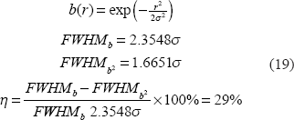
Diagram for linear and nonlinear operations involved in BOLD fMRI. The complex modulo operation imposes a nonlinearity in T2^* magnitude image acquisition and the complex argument operation may cause a weak nonlinearity in T2^* phase image acquisition. In the small angle regime, the T2^* magnitude image assumes a quadratic nonlinearity in relation to the susceptibility source, and the T2^* phase image assumes a linear conformance with the fieldmap.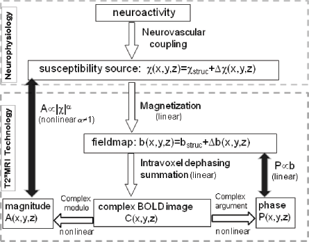

Spatial transformations

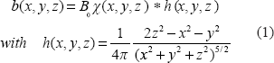
As shown in Figure 1, the T2^*MRI module (in the lower box) is decomposed into 2 steps in the imaging process. The first step is to establish a 3D fieldmap via magnetization in a main field B₀ that can be expressed by a 3D convolution^4,5 by

$$\begin{array}{l}b(x,y,z)=B_0\chi (x,y,z)*h(x,y,z)\\ \begin{array}{ll}with\hfill & h(x,y,z)=\frac{1}{4\pi }\frac{2z^2-x^2-y^2}{{(x^2+y^2+z^2)}^{5/2}}\hfill \end{array}\end{array}$$

(1)

where ^* denotes 3D convolution, h(x, y, z) the point magnetic dipole field, and b(x, y, z) the fieldmap (the z-component of magnetization in addition to B₀). From the perspective of an imaging system, b(x, y, z) is morphologically different from χ(x, y, z) due to h(x, y, z) ≠ δ(x, y, z). That is, a convolution with a finite point spread function (a nonpoint kernel) will cause a spatial spread effect on the image transformation. For a typical imaging system (such an optical imaging system) that assumes a nonnegative and unimodal kernel, the spatial spread effect causes morphological mismatch or distortion. Because of the abnormal bipolar-valued anisotropic distribution^5,6 of the 3D dipole kernel in Equation (1), the 3D convolution exhibits both spatial spread effect and spatial derivative effect, ⁴ which produces a complicated morphological change. In particular, the distance-decaying spatial spread function of the dipole kernel causes spatial blurring (morphological dilation), the anisotropy causes asymmetry, the bipolar distribution causes spatial derivative effect (textural enhancement effect), and the zeros surface causes an orientation effect (magic angle effect). ⁵ In summary, the 3D convolution in Equation (1) dictates a morphological mismatch between the fieldmap and the χ source, as termed dipole effect.

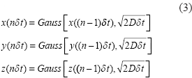
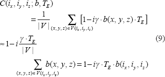
The second step is an intravoxel dephasing average for signal and image formation. In the absence of diffusion, the intravoxel static dephasing signal can be expressed by^3,20

$$C(i_x,i_y,i_z;b,T_E)=\frac{1}{\left|V\right|}\sum _{(x^{\prime },y^{\prime },z)\in V(i_x,i_y,i_z)}exp[-i\gamma \cdot b(x,y,z)\cdot T_E]$$

(2)

where V(i _x , i _y , i _z ) denotes a voxel at (i _x , i _y , i _z ), and |V| the voxel size, and T _E the echo time. Note that we use (x, y, z)-notation to represent the conceptually continuous field of view (FOV) space (digitally implemented in a fine grid large support matrix) and (i _x , i _y , i _z )-notation to represent the voxelized FOV space (spatially sampled or partitioned into a multivoxel matrix, also called voxelization ³ ). The (x, y, z)-notation is used for the FOV vasculature depiction and the fieldmap calculation and the (i _x , i _y , i _z )-notation is used for FOV partition and multivoxel image formation (manipulation of (i _x , i _y , i _z )- indexed voxels) (as will be used to describe the volumetric BOLD fMRI simulation later). It is noted that in a T2^* complex image in Equation (2) we include the explicit parameters of echo time T _E and field value b to remind the dependence upon the T2^*MRI protocol setting, which should be specified in numerical simulations (see later).

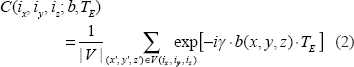
In presence of diffusion, the intravoxel dephasing signal can be expressed by^21,22

$$C(i_x,i_y,i_z;b,T_E)=\frac{1}{\left|V\right|}\sum _{(x,y,z)\in V(i_x,i_y,i_z)}\left[-i\gamma \cdot \sum _n^{N}b(x(n\delta t),y(n\delta t),z(n\delta t))\cdot \delta t\right]$$

with T_E = Nδt

$$\begin{array}{l}x(n\delta t)=Gauss\left[x((n-1)\delta t),\hspace{0.17em}\sqrt{2D\delta t}\right]\\ y(n\delta t)=Gauss\left[y((n-1)\delta t),\hspace{0.17em}\sqrt{2D\delta t}\right]\\ z(n\delta t)=Gauss\left[z((n-1)\delta t),\hspace{0.17em}\sqrt{2D\delta t}\right]\end{array}$$

(3)

where D denotes the water molecule diffusion coefficient (D = 10^-5 cm²/s), δt the diffusion time step, and Gauss (x, σ) denotes a Gaussian distribution with mean x and standard deviation σ. For brain soft tissue, the water molecule diffusion can be modeled by unrestricted Gaussian random motion (with an isotropic diffusion coefficient D). ²¹

Upon the acquisition of the complex dataset C(i _x , i _y , i _z ; T _E ), we can calculate its magnitude loss (simply called magnitude henceforth) and phase angle accrual (simply called phase henceforth) during T _E by

$$\{\begin{array}{c}A(i_x,i_y,i_z;T_E)=1-\left|C(i_x,i_y,i_z;T_E)\right|/\left|C(i_x,i_y,i_z;T_E=0)\right|\\ =1-\left|C(i_x,i_y,i_z;T_E)\right|\\ P(i_x,i_y,i_z;T_E)=\angle \left[C(i_x,i_y,i_z;T_E)/C(i_x,i_y,i_z;T_E=0)\right]\\ =\angle C(i_x,i_y,i_z;T_E)\end{array}$$

(4)

where |C(i _x , i _y , i _z ; T _E = 0)| = 1 and $\angle C(i_x,i_y,i_z;T_E=0)=0$ are assumed. Conventionally, A(i _x , i _y , i _z ; T _E ) is considered as an “image” of the susceptibility source χ(i _x , i _y , i _z ) (a voxelized version of χ(x, y, z)) acquired by T2^*MRI with a gradient echo time T _E . The intravoxel dephasing formulas in Equations (2) and (3) for complex voxel signal formation are linear due to the fact that a vector sum or a complex addition is linear (the linearity associated with multiresolution intravoxel dephasing summation has been described by “rebinning invariance” ¹⁶ ). Nevertheless, the complex modulo operation for magnitude calculation and the complex argument operation for phase calculation in Equation (4) are no longer linear: the magnitude calculation suffers a strong nonlinearity and the phase calculation suffers a weak nonlinearity in the small phase angle regime (see later).

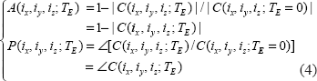
Nonnegative magnitude image

It is obvious that the magnitude of a complex number is nonnegative. Since the field value plays a factor in the phase angle of the complex BOLD signal, the BOLD signal resulting from a negative field value is equivalent to a conjugate of that from a positive field value. That is, the signal magnitudes resulting from the positive and negative fields are degenerated, as expressed by

$$\begin{array}{l}\left|C(i_x,i_y,i_z;b)\right|=\sqrt{conj[C(i_x,i_y,i_z;b)]\cdot C(i_x,i_y,i_z;b)}\\ =\sqrt{C(i_x,i_y,i_z;-b)\cdot C(i_x,i_y,i_z;b)}\\ =\sqrt{C(i_x,i_y,i_z;-b)\cdot conj[C(i_x,i_y,i_z;-b)]}\\ =\left|C(i_x,i_y,i_z;-b)\right|>0\end{array}$$

(5)

where conj denotes a complex conjugate operation, that is conj[exp(-iφ] = exp(iφ). It is seen that the T2^* magnitude image cannot discriminate a negative field (χ < 0) from a positive field (χ > 0). We describe the phenomenon that either b or -b produces the same magnitude by a term of field sign degeneracy. For dynamic functional imaging, a neuronal activity may simultaneously cause a positive response at one point and a negative response at another point on a static structural background (baseline). Suppose a spatial superimposition for χ-induced field perturbation, b = b_struct+Δb, where b_struct denotes static structural background (baseline) and Δb the dynamic BOLD field perturbation, we can factorize the complex voxel signal by

$$\begin{array}{l}C(i_x,i_y,i_z;b_{struct}+\Delta b)=C(i_x,i_y,i_z;b_{struct})\cdot C(i_x,i_y,i_z;\Delta b)\\ s\cdot t\cdot b_{struc}(x,y,z)=b_{struc}(i_x,i_y,i_z)\forall (x,y,z)\in V(i_x,i_y,i_z)(\text{intravoxel}\hspace{0.17em}\text{uniformity})\end{array}$$

(6)

∈ V(i _x , i _y , i _z ) (intravoxel uniformity)

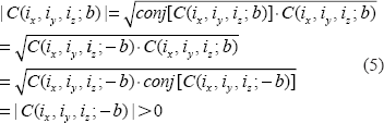
Then we have,

$$\begin{array}{l}\left|C(i_x,i_y,i_z;b_{struct}-\Delta b)\right|=\left|C(i_x,i_y,i_z;b_{struct})\right|\cdot \left|C(i_x,i_y,i_z;-\Delta b)\right|\\ =\left|C(i_x,i_y,i_z;b_{struct})\right|\cdot \left|C(i_x,i_y,i_z;\Delta b)\right|\\ =\left|C(i_x,i_y,i_z;b_{struct}+\Delta b)\right|>0\end{array}$$

(7)

which indicates that T2^* magnitude image cannot discriminate a negative field change (Δb < 0) from a positive change (Δb > 0), which has been described by a pitfall of magnitude non-negativity for brain imaging. ⁶ It is noted that Equations (6) and (7) hold for a cortical voxel that has no intravoxel structure (as expressed by uniform intravoxel interior in Equation (6), where b _struc (i _x , i _y , i _z ) ≠ b _struc (i’ _x , i’ _y , i’ _z ) for (i _x , i _y , i _z ) ≠ (i’ _x , i’ _y , i’ _z ) represents the intervoxel difference).

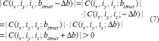
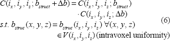
The complex signal factorization in Equation (6) and the field sign degeneracy in Equation (7) may become invalid due to intravoxel substructure and diffusion effect. Anyway, the relations in Equations (6) and (7) provide approximate formulations for perceiving the behaviors of T2^* magnitude signal with respect to BOLD χ response. We should point out that the concept of magnitude's nonnegativity is different from that of dynamic negative BOLD signal change: for the former is said to a single T2^* magnitude signal that assume a nonnegative value (no matter how the χ source or the field changes), and the later is to the relative change between 2 nonnegative T2^* magnitude signals acquired at 2 time points or 2 states (an active state in reference to a baseline state). That is, a negative BOLD signal change results from the post-processing on a timeseries of nonnegative T2^* magnitude dataset (raw data), a decrease in signal magnitude among 2 states. In this work, we do not address the negative behavior of dynamic BOLD signals.

Source-image relationship in the small phase angle regime

To enable the theoretical analysis on the T2^* complex signal, we adopt an approximation condition of small phase angle regime^4,6 that is expressed by

$$\begin{array}{cc}exp(i\varphi )\approx 1+i\varphi & \text{for}\left|\varphi \right|<<\pi \end{array}$$

(8)

which is essentially a linear phase approximation. Under the condition in Equation (8), we can reformat Equation (2) into

$$\begin{array}{l}C(i_x,i_y,i_z;b,T_E)=\frac{1}{\left|V\right|}\sum _{(x,y,z)\in V(i_x,i_y,i_z)}[1-i\gamma \cdot b(x,y,z)\cdot T_E]\\ \approx 1-i\frac{\gamma \cdot T_E}{\left|V\right|}\sum _{(x,y,z)\in V(i_x,i_y,i_z)}b(x,y,z)=1-i\gamma \cdot T_E\cdot b(i_x,i_y,i_z)\end{array}$$

(9)

where the (i _x , i _y , i _z )-notation denotes intravoxel average (suppression of voxel substructure). As a result, the magnitude and phase of BOLD fMRI are given by

$$\{\begin{array}{c}A(i_x,i_y,i_z;T_E)\approx 1-|1-i\gamma T_E\cdot b(i_x,i_y,i_z))|\\ =\frac{1}{2}{[\gamma T_E\cdot b(i_x,i_y,i_z)]}^2(nonlinear)\\ P(i_x,i_y,i_z;T_E)\approx -\gamma T_E\cdot b(i_x,i_y,i_z)(linear)\end{array}$$

(10)

which shows that the magnitude is a nonlinear (quadratic) function of echo time (T _E ) and voxel field (b(i _x , i _y , i _z )), whereas the phase takes on a linear function of T _E and b(i _x , i _y , i _z ). In other words, the T2^* magnitude is always nonlinearly related to the fieldmap, with the least nonlinearity of quadratics in the small phase condition, which cannot be linearly approximated anyway. For example, the quadratic suffers a field sign degeneracy, which manifests as negative inverse artifact, that is a strong nonlinearity. In comparison, the linearity between the phase and the fieldmap with a scale factor indicates that there is no information loss during the step from fieldmap to the T2^* phase acquisition (in Fig. 1), thus promising the brain χ tomography via T2^* phase image. ¹⁹

As the phase angle increases, the small angle condition in Equation (8) is invalid, and higher orders of [γT _E b(i _x ,i _y ,i _z )] will be introduced into the formulas in Equation (10) thereby causing more nonlinearity in T2^* magnitude nonlinearity. A large phase angle (|P|>π) may cause phase wrapping phenomenon, which is of a nonlinear behavior. In such case, a phase unwrapping preprocessing is necessary for fieldmap calculation and χ reconstruction.

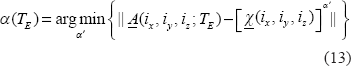
Empirical characterization of source-image nonlinearity

In order to compare the 3D patterns of χ(i _x , i _y , i _z ) and A(i _x , i _y , i _z ; T _E ), we normalize their ranges to [0,1] as follows

$$\begin{array}{l}\underset{\_}{\chi }(i_x,i_y,i_z)=\frac{\left|\chi (i_x,i_y,i_z)\right|-{\left|\chi \right|}_{min}}{{\left|\chi \right|}_{max}-{\left|\chi \right|}_{min}}\\ \underset{\_}{A}(i_x,i_y,i_z;T_E)=\frac{A(i_x,i_y,i_z;T_E)-A_{min}}{A_{max}-A_{min}}\end{array}$$

(11)

which is referred to as [0,1]-normalization. It is noted that the nonnegative |χ| is used to define the [0,1]-normalization such that it allows us to compare a negative response source (χ < 0) with its nonnegative magnitude image. We suggest to relate the [0,1]-normalized source and the [0,1]-normalized images by an empirical α-power model, that is

$$\underset{\_}{A}(i_x,i_y,i_z;T_E)={\left[\left|\underset{\_}{\chi }\right|(i_x,i_y,i_z)\right]}^{\alpha (T_E)}+\epsilon (i_x,i_y,i_z;T_E)$$

(12)

for which we calculate the empirical parameter α by an optimal fitting

$$\alpha (T_E)=\underset{{\alpha }^{\text{'}}}{argmin}\{\Vert \underset{\_}{A}(i_x,i_y,i_z;T_E)-{[\underset{\_}{\chi }(i_x,i_y,i_z)]}^{{\alpha }^{\_}}\Vert \}$$

(13)

where we retain the parameter T _E to remind us that the nonlinearity and error fitting are T _E -dependent, as will be demonstrated in our simulations.

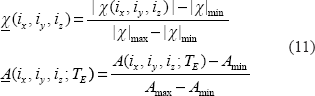
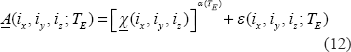
Upon α values in Equation (12), we can describe the morphological relationship between the T2^* magnitude image and the χ source in 3 possible categories: shrinkage, replica, and dilation as expressed by

$$\underset{\_}{A}(x)={\underset{\_}{\chi }}^{\alpha }(x)\{\begin{array}{l}<\underset{\_}{\chi },\hspace{0.17em}\text{for}\hspace{0.17em}\alpha >1\hspace{0.17em}(\text{shrinkage})\hfill \\ =\underset{\_}{\chi },\hspace{0.17em}\text{for}\hspace{0.17em}\alpha =1\hspace{0.17em}\hspace{0.17em}(\text{replica})\hfill \\ >\underset{\_}{\chi },\hspace{0.17em}\text{for}\hspace{0.17em}\alpha \hspace{0.17em}<1\hspace{0.17em}\hspace{0.17em}(\text{dilation})\hfill \end{array}$$

(14)

Therefore, we may use the exponent a value to numerically characterize the T2^* magnitude nonlinearity and morphological mismatch (α ≠ 1). On the other hand, for a T2^* phase image, which bears a well-known dipole effect that makes a striking pattern mismatch between the χ source and the T2^* phase image, the attempt to render pattern match therewith does not make sense. Instead, we are concerned with the pattern match between T2^* phase image and the χ-induced fieldmap in the small phase regime.

Pattern mismatch measures

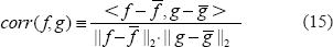
Spatial correlation

We propose a measure of spatial correlation to numerically characterize the similarity of 2 3D patterns: f(x, y, z) and g(x, y, z), that is,

$$\text{corr}(f,g)\equiv \frac{<f-\overline{f,}g-\bar{g}>}{{\Vert f-\bar{f}\Vert }_2\cdot {\Vert g-\bar{g}\Vert }_2}$$

(15)

where <, > denotes inner product, and ${\Vert \cdot \Vert }_2$ the L₂-norm. Since corr(f, g) ≤ 1 (with corr(f, g) = 1 for replica), we can measure the mismatch between f and g by 1-corr(f, g). As reported in our previous publications,³⁵ we are concerned with the spatial match between T2^* magnitude and magnetic susceptibility source (denoted by corr(A, |χ|)) and with that between T2^* phase and fieldmap (denoted by corr(P, b)). The spatial correlation also provides a measure of nonlinear relationship between f and g, as expressed by

$$\text{corr}(f,g)\{\begin{array}{ll}=1\hfill & (\text{linearity})\hfill \\ \ne 1,\hfill & (\text{nonlinearity})\hfill \end{array}$$

(16)

Full width at half maximum

For a spherical source and its image, we suggest a shape measure described in terms of full width at half maximum (FWHM), which is defined for a 1D scanline profile. For a 2D cross-section and a 3D volume, the FWHM manifests as the diameter of a disk and a sphere. To characterize the morphological change of the round blob under BOLD fMRI, we suggest a FWHM change percentage as defined by

$${\eta }_A=\frac{FWH{M}_{\chi }-FWH{M}_A}{FWH{M}_{\chi }}\times 100\%$$

(17)

For a digital spherical graded distribution after [0,1]-normalization, we can calculate the 3D FWHM by

$$\begin{array}{c}FWH{M}_{\lambda }=2{\left[\frac{3}{4\pi }\sum _{(i_x,i_y,i_z)\in FOV}\lambda (i_x,i_y,i_z)\ge \frac{1}{2}\right]}^{-1/3}\\ \text{for}\hspace{0.17em}\lambda =\{\underset{\_}{\chi },\underset{\_}{A}\}\end{array}$$

(18)

which is construed a diameter of a 3D ball (resulting from an isosurface at isovalue = 1/2 (note that a 3D ball with diameter d produces a volume by 4π(d/2) ³ /3). A positive and negative fraction in Equation (17) implies a shape shrinkage and dilation, respectively. There are many factors responsible for FWHMs, which we are concerned with in our simulations, including echo time, voxel size, vessel size, and field strength.

Suppose a Gaussian-shaped fieldmap; we have

$$\begin{array}{c}b(r)exp\left(-\frac{r^2}{2\sigma }\right)\\ FWH{M}_b=2.3548\sigma \\ FWH{M}_{b^2}=1.6651\sigma \\ \eta =\frac{FWH{M}_b-FWH{M}_{b^2}}{FWH{M}_{b}2.3548\sigma }\times 100\%=29\%\end{array}$$

(19)

which indicates that the intravoxel dephasing for T2^* magnitude image formation from a fieldmap suffers a morphological shrinkage of 29%. This estimation is valid for a Gaussian-shaped fieldmap in the small phase angle regime and in the absence of diffusion. For a practical situation, a χ blob may assume a Gaussian-shaped distribution but its fieldmap will not due to spatial derivative effect of the 3D convolution with a bipolar-valued anisotropic kernel (in Equation (1)). Moreover, the diffusion absence the morphological shrinkage calculation in Equation (19) results in an overestimate. This is because the diffusion effect plays a morphological dilation (diffusion blurring), which will reduce the shrinkage effect to some extent (as will be demonstrated with numerical simulations). We consider η = 29% as a theoretical estimation of the morphological shrinkage of a static dephasing T2^* magnitude image from a Gaussian-shaped fieldmap due to a quadratic nonlinearity. The morphological shrinkage from a Gaussian-shaped χ source to T2^* magnitude image formation will be empirically characterized by numerical simulations.

Numerical Simulations and Phantom Experiment

Nonlinearity of BOLD fMRI signal

Because the goal of BOLD fMRI is to measure the bulk blood χ perturbation of a hemodynamic process in response to a brain activity, we can perform numerical simulations to observe the nonlinear behavior of BOLD signals. We start by configuring a cortical voxel with a random vessel network,^23,24 then calculate the intravascular blood χ perturbation as expressed by

$$\begin{array}{l}\chi (x,y,z;t)={\chi }_{struc}(x,y,z)+\Delta \chi (x,y,z;t)\\ \text{with}\hspace{0.17em}\Delta \chi (x,y,z;t)={\chi }_{do}\cdot [1-Y(t)]\cdot Hct\cdot V(x,y,z;t)\\ \text{and}\hspace{0.17em}V(x,y,z)=\{\begin{array}{l}1,(x,y,z)\hspace{0.17em}\text{in}\hspace{0.17em}\text{vessel}\hfill \\ 0,\hspace{0.17em}\text{else}\hfill \end{array}\end{array}$$

(20)

where χ _do = 0.27 ppm × 4π (SI unit), Y = 0.6, Hct = 0.4 for a typical human brain state, ¹⁷ V(x, y, z; t) denotes a binary volume representing a cortical voxel (filled with random vasculature in (x, y, z)-notation representation), and the time t is reserved as a parameter to represent the dynamics in blood volume (via V(x, y, z; t)) and in oxygenation level (via Y(t)) during a neuronal activity ³ For dynamic functional imaging by T2^*MRI, the event time t is referred to as the snapshot time point, which is conceptually different from the protocol echo time T _E .

The magnetization of a χ-expressed brain tissue state in a main field B₀ causes a fieldmap disturbance as expressed by

$$\begin{array}{c}b(x,y,z;t)=B_0[{\chi }_{struc}(x,y,z)+\Delta \chi (x,y,z;t)]*h(x,y,z)\\ =b_{struc}(x,y,z)+\Delta b(x,y,z;t)\end{array}$$

(21)

where the fieldmap is decomposed into 2 additional parts: static structural contribution and dynamic functional contribution. In our numerical simulation, we assume uniform extravascular χ distribution, that is χ _struc (x, y, z) = const and b _struc (x, y, z) = const. For dynamic BOLD fMRI simulation, we calculate a 3D complex-valued T2^* image at each snapshot time, thus omitting the time variable t henceforth.

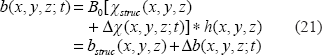
Based on an intravoxel vasculature model for cortex voxel configuration,^21,25,26 we implement BOLD voxel signal simulation by the following parameter settings: voxel size = 320 × 320 × 320 micrometer ³ (voxel matrix 512 × 512 × 512), intravoxel vessel radius = 3 micrometer, bfrac = 2%, B₀ = 3T, T _E = 30 milliseconds, Δχ _xunc = -1.5:0.1:1.5 ppm (spanning a range of [-1.5,1.5 ppm] with an increment of 0.1 ppm), χ _struc = -1 ppm (uniform extravascular space). Since a uniform intravoxel background (baseline) has no contribution to intravoxel dephasing, the BOLD voxel signal is invariant to an offset (χ _struc = const). The numerical simulations show the magnitude and phase behavior of BOLD fMRI signals in Figure 2 with respect to a diverse of parameters {T _E , Δ_χ, B₀, static/diffusion}. It is observed that the BOLD magnitude signal exhibits a strong nonlinearity in Figure 2(a), conspicuous for the nonnegativeness with respect to the bidirectional χ perturbations (sign degeneracy). In the small angle regime, around the origin at Δχ = 0 in Figure 2(a), the BOLD magnitude assumes a quadratic transformation on Δχ (a parabola), which agrees with the theoretical prediction in the small angle regime (in Equation (10)). However, the BOLD phase exhibits a good linearity with respect to Δχ (in Fig. 2(b)) and to T _E (in Fig. 2(d)), which is desirable for brain χ reconstruction from T2^* phase image. It is noted that the linear phase behaviors in Figures 2(b) and 2(d) are observed in the phase unwrapping condition (<0.5 rad).

Figure 2

Numerical simulations on the nonlinear behaviors of T2^*MRI complex signal with respect to magnetic susceptibility perturbation (Δχ = [-1.5,1.5 ppm]), echo time (T _E = [0,30] milliseconds), field strength (B₀ = [0.5,7] Tesla in legend) and for 2 scenarios: diffusion-present and diffusion-absent dephasings, (a) and (c) for magnitude signals, and (b) and (d) for phase signals.

Morphological shrinkage of volumetric BOLD fMRI

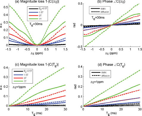
The digital geometry for a cortical FOV is represented by a 3D support matrix in size of 2048 × 2048 × 2048 with 1-micrometer grid resolution (in (x, y, z)-notation representation). In order to evaluate the statistical fluctuation resulting from vasculature dependence,^3,26 the FOV is filled with beads (radius = 3 micrometer for the human dominant cerebral cortex vasculature) demonstrated in Figure 3. It is noted that the difference between the cortical FOV configuration in Figure 3 and that reported in our previous publication ³ is that we replace the random cylindrical vessels with random spherical beads in order to have a good control of bfrac = 2% over voxels in the FOV. The 3D BOLD Δχ source is formed by a spatial modulation of cortical vasculature and a local Gaussian-shaped neuroactivity in the cortical FOV (called a linear neurovascular coupling ³ ). The 3D fieldmap Δb(x, y, z) is calculated by Equation (21), which is represented by a matrix (in size of 2048 × 2048 × 2048) as large as the support matrix of FOV. With 3 voxel sizes, 32 × 32 × 32, 64 × 64 × 64, and 128 × 128 × 128 micrometer ³ , we can partition the large support matrix (2048 × 2048 × 2048) into small matrices in size 64 × 64 × 64, 32 × 32 × 32 and 16 × 16 × 16 (in (i _x , i _y , i _z )-notation representation) thus implementing volumetric BOLD fMRI simulations at 3 resolutions. In Figures 3(c1) and 3(c2), we demonstrate the central slices of the FOV at 2 resolutions.

Figure 3

A Gaussian-shaped susceptibility blob in a cortical FOV for BOLD fMRI simulation. (a) A central slice of the bead-laden FOV that is represented by a large support matrix in size of 2048 × 2048 × 2048 and under the spatial modulation by a Gaussian-shaped neuroactivity blob. (b) A blowout display of a bead-laden voxel in size of 64 × 64 × 64 for FOV partition. With voxel size of 32 × 32 × 32 and 64 × 64 × 64, the FOV is portioned into a matrix of 64 × 64 × 64 in(c1) and 32 × 32 × 32 in (c2), respectively.

The numerical simulation allows us to calculate intravoxel dephasing images for 2 scenarios: diffusion-absent dephasing image (also called static image) by Equation (2) and diffusion-present dephasing image by Equation (3). In Figure 4 are shown the 3D voxelized χ source and the fieldmap, in form of matrix of size 32 × 32 × 32 (in (i_x, i_y, i_z)-notation representation) resulting from voxelization by a voxel size of 64 × 64 × 64 (in (x, y, z)-notation representation). In Figure 5, we show the central z-slices of the T2^* magnitude images calculated in absence and presence of diffusion and the scanline profiles for quantitative scrutiny. It is seen from Figures 4 and 5 that the T2^* magnitude exhibits a shape shrinkage in relative to its susceptibility blob. The definition of FWHM is also illustrated in Figure 5(b).

Figure 4

Montage displays of 3D 64 × 64 × 64 data matrices for i _z = 3:32 slices with i _z = 32 at the central z-slice. (a) 3D susceptibility Δχ(64,64,64) in units of ppm, (b) BOLD fieldmap Δb(64,64,64) in units of ppmT, (c) T2^* magnitude A(64,64,64) with dimensionless ratio units, and (d) T2^* phase P(64,64,64) in units of radian. It is seen that the T2^* magnitude image resembles the susceptibility source but with a morphological shrinkage and T2^* phase image is almost identical to the fieldmap.

Figure 5

Demonstration of morphological shrinkage in T2^*MRI with the central z-slice images. (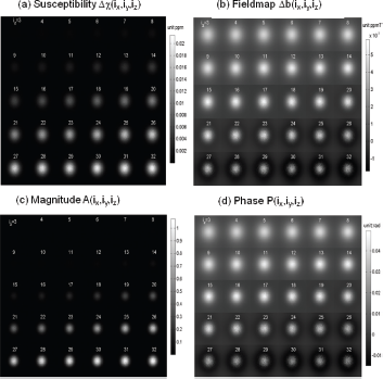a) The susceptibility source (at central z-slice); (b) the magnitude image of T2^*MRI simulation in absence of diffusion; (c) the phase image in presence of diffusion; (d) profiles along the scanlines (as marked in (a)) with illustrations of 1D FWHM. All the images in (a), (b), and (c) are normalized to [0,1] and displayed with the same greylevel bar.

In terms of spatial correlation between the predefined χ source and the calculated T2^* image, we can numerically characterize the effects of diffusion and echo time on volumetric BOLD fMRI. For the particular simulations in Figure 4, we present the diffusion effect (with dotted lines) and echo time effect (with abscissa) on volumetric BOLD fMRI in Figure 6, where corr(A, χ) is for source/image match and corr(P, b) is for phase/fieldmap match. It is observed that, in absence of diffusion, corr(P, b) = 1.00 and is basically invariant to T _E , and corr(A, χ) increases for long T _E ; in presence of diffusion, corr(P, b) suffers a slight drop (≍0.99) for short T _E (<10 milliseconds) then approaches 1 for long T _E (>15 milliseconds), and corr(A, χ) remains at 0.91 that is basically invariant to T _E (indicating the source/image mismatch is almost independent of T _E ). 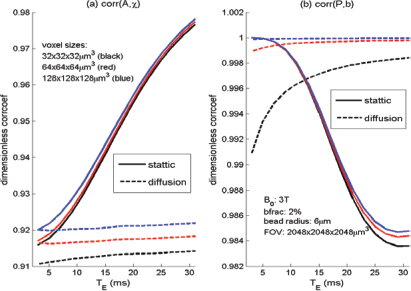In Figure 7, we demonstrate the effect of spatial resolution on corr(A, χ) and corr(P, b), which shows that high spatial resolution (small voxel size) will decrease the match slightly.

Figure 6

Effects of diffusion and echo time on the spatial match between the T2^* magnitude image and the susceptibility source, and on that between the T2^* phase image and the fieldmap.

Figure 7

Spatial correlation measures of (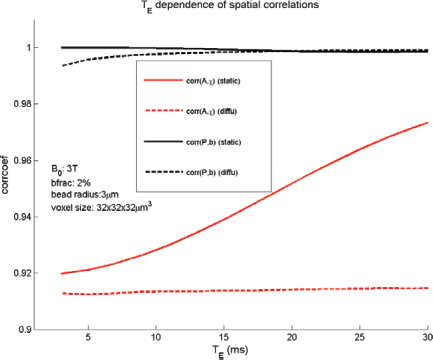a) corr(A, χ) and (b) corr(P, b) of volumetric BOLD fMRI simulations for a FOV filled with 6-micrometer-raidus beads under the setting of a range of echo time (T _E = [0,30] milliseconds), 3 resolutions = {32, 64, 128} micrometer, and 2 scenarios: diffusion-absent and diffusion-present dephasing images (see legend).

Based on the volumetric BOLD fMRI simulations with a Gaussian-shaped susceptibility blob (see Fig. 3) for a variety of parameters, we calculate the exponent a and the residue error ε by Equation (13). In Figure 8, we show that both α and ε are affected by the following aspects: static and diffusion (see legend for solid and dotted lines), different spatial resolution (marked by line colors), different echo times (with respect to the abscissa), and different vessel sizes (3 micrometer in (a1) (b1) and 6 micrometer in (a2) and (b2)).

Figure 8

Simulation results of α-power model with respect to diffusion presence (in dotted lines) and diffusion absence (in solid lines), t3 resolutions (32 micrometer in black, 64 micrometer in blue, and 128 micrometer in red), vessel size (radius = 3 mircometer at left-hand column and radius = 6 micrometer at right-hand column), and echo time (the abscissa).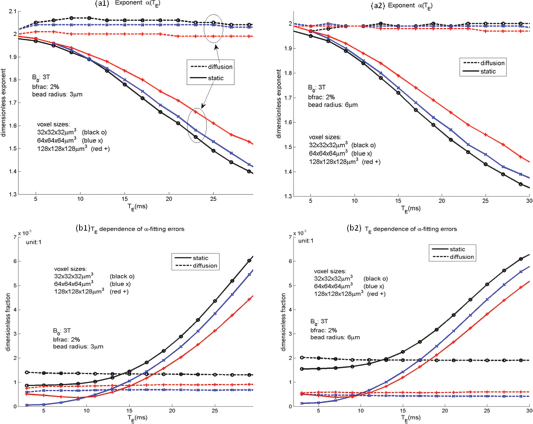

In presence of spin diffusion, we obtain that the T2^* magnitude is approximated by a 2-power transformation on the susceptibility source and that exponent a is invariant to echo time and slightly varies with the imaging spatial resolution (in Figs. 8(a1) and 8(a2)), and that the fitting errors are smaller for lower resolution and are invariant to echo time (in Figs. 8(b1) and 8(b2)). In the absence of spin diffusion (static dephasing), the a value decreases (see Figs. 8(a1) and 8(a2)) and the fitting error increases (see Figs. 8(b1) and 8(b2) for T _E > 15 ms) with respect to echo time.

According to Equation (12), the 2-power nonlinear transformation will exhibit a morphological shrinkage (|χ| ² < |χ| for |χ| < 1). We calculate the FWHM change percentage by Equations (17) and (18). The results are shown in Figure 9, which indicate that the T2^* magnitude shrinkage in reference to the susceptibility source shape is in the range of 25% to 30%, and that the shrinkage slightly reduces as the resolution decreases. For static dephasing signals, the shrinkage gradually reduces as the echo time prolongs, and it disappears (η = 0) at T _E = 30 milliseconds. It is noted that the zero-shrinkage scenario corresponds to α ≍ 1.4 in Figures 8(a1) and 8(a2), implying that there is an interplay between the magnitude nonlinearity and the 3D dipole effect in the absence of diffusion that provides some cancellation of the morphological change. Because a practical T2^*MRI cannot avoid the ubiquitous diffusion phenomenon, the zero-shrinkage case is an approximation when the diffusion effect is insignificant (ie, a static dephasing condition). It is also noted that, in the absence of diffusion effect, the static dephasing T2^* magnitude image exhibits a morphological dilation for long echo times (T _E > 30 milliseconds), which requires further study.

Figure 9

Morphological shrinkage in terms of FWHM percentage calculated by (d _x –d _A )/d _A , with d _x = FWHM and d _A = FWHM_A for (a1) for radius = 3 micrometer, and (b1) for radius = 6 micrometer.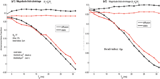

Phantom experiment

In Figure 10, we provide a phantom experiment to demonstrate the dipole effect and morphological shrinkage in T2^*MRI. The phantom is made of a large cylinder water container (diameter = 950 mm) with a small plastic tube (diameter = 15 mm) at the central axis. The plastic tube is filled with diluted gadolinium (Gd) solution (dilution = 0.4 mL/30 mL with clinical Gd dye in water), which provides a tube-shaped uniform χ distribution in contrast with the surrounding water (ground truth: a cylindrical χ map). The phantom was scanned in a Siemens 3T Trio scanner with a complex EPI sequence, with standard BOLD fMRI parameters (T = 29 ms, FOV = 224 × 224 × 112 mm³ (matrix: 64 × 64 × 32), voxel size = 3.5 × 3.5 × 3.5 mm³, flip angle = 75°, zero oblique: B₀┴ tube axis). This static phantom experiment produces a single complex T2^* image (magnitude and phase images are shown in Figs.10(a) and 10(b)). It is observed that the magnitude image in Figure 10(a) bears a central dip at the Gd-tube, indicating an edge effect, and that the phase image in Figure 10(b) suffers a striking dipole effect. From the 3D phase image, we reconstructed a 3D χ map by CIMRI. ⁴ The corresponding cross section of the reconstructed cylindrical χ map is shown in Figure 10(c). By comparing (c) with (b), we observe the removal of the dipole effect by 3D deconvolution (core technology of CIMRI). By comparing (c) with (a), we observe a slight morphological shrinkage of T2^* magnitude in relative to the χ source. We also provide scanline profiles in Figure 10(d), with a scanline along the Gd-tube diameter as marked in (a)).

Figure 10

A phantom experiment. The phantom is made of a large cylindrical water container diameter = 950 mm) and a small Gd-filled plastic tube (diameter = 15 mm) at the center of water tank. The Gd-tube phantom offers a tube-shaped cylindrical susceptibility distribution (the χ truth). (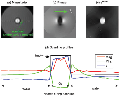a) T2^* magnitude image, (b) T2^* phase image, (c) reconstructed χ map, and (d) scanline profiles (the scanline is defined in (a)). The dipole effect is observed in the T2^* phase image, manifesting as strong positive and negative field values at the tube boundary. A slight shape shrinkage is observed in the T2^* magnitude image by comparing it with the reconstructed χ map (or with the known truth: rectangle form in (d)).

We utilize a Gd-tube experiment, instead of a spherical graded χ phantom due to the significant challenge in manufacturing such a phantom. As such, our phantom experiment has the following limitations:

1. (1)

The uniform Gd solution inside the tube provides a cylindrical χ map in contrast with the surrounding water, and, thus, we cannot compare the phantom morphological shrinkage with the results from BOLD fMRI simulations with a Gaussian χ model (as reported in this paper) because a jump at a boundary behaves differently from a curved slope.

(2)

The experiment also suffers from imperfect field shimming (an experimental systematic error) as observed on the uneven levels at the left-hand side and right-hand side of T2^* magnitude and reconstructed χ map in Figure 10(d), which is responsible for the unexpected slope in the reconstructed χ map inside the tube.

(3)

The straight slope edges at the tube boundary (in comparison with the ideal sharp rectangular edges) are due to the low resolution FOV sampling (3.5 mm voxel size) and possibly the wall thickness of the plastic tube (=1 mm).

In spite of these circumstances, the phantom experiment in Figure 10 enables us to demonstrate the morphological mismatch between the χ source and T2^* magnitude and phase images, as well as the dipole effect removal by CIMRI, thereby providing experimental support to the theory in Section 2 to some extent.

Discussion

The fundamental assumption of BOLD fMRI modality assumes that the T2^* magnitude is an image of a brain activity (via a phenotypic expression of vascular blood χ perturbation). Based on numerical simulations, as reported in this paper and in our previous publications, ³ we have found that the T2^* magnitude image is not an exact digital reproduction of the internal χ source (corr(A, χ) ≍ 0.90). In this sense, a T2^* magnitude image cannot be considered as tomographic image of the χ source. In this paper, we attempt to understand the morphological mismatch (corr((A, χ) < 1) by looking into insights of the T2^*MRI technology.

We describe T2^*MRI by 2 steps: 3D convolutional magnetization and intravoxel dephasing detection. The 3D convolution is a linear transformation, but its spatial spread property (or local average within the extent of convolution kernel) dictates a morphological mismatch. The intravoxel dephasing for T2^* complex signal formation only involves complex signal addition (average),^16,21,25 which is a linear process for complex number addition or vector addition. However, the calculations of T2^* magnitude and phase from a T2^* complex signal are nonlinear. Specifically, the complex modulo operation for calculating the magnitude of a complex number is nonlinear. Especially, the magnitude calculation suffers a field sign degeneracy: a positive field value Δb and a negative field value -Δb produce the same T2^* magnitude. In general, the nonlinearity of T2^* magnitude in relation to its fieldmap and to its χ source is difficult to analytically formulate. In the small phase angle regime (γT _E b<<π) in Eq. (8), we show that the T2^* magnitude is related to the fieldmap by a quadratic transformation in Equation (10). It is understood that as the phase angle of spin precession in Equations (2) and (3) increases, the small angle condition in Equation (8) is no longer held (for example, γ T _E b ≍ π resulting from long echo time T _E and high field value b). As a result, higher-order terms ((γT _E b). ⁿ for n > 2) are introduced in Equation (8), and the T2^* magnitude calculation bears higher nonlinearity. We consider the quadratic nonlinearity in Equation (10) as the least nonlinearity for T2^* magnitude formation in the small phase angle regime, which cannot be linearly approximated anyway. In particular, the least quadratic nonlinearity bears a field sign degeneracy (magnitude nonnegativity). Together with the diffusion effect, the quadratic nonlinearity explains the empirical exponent α ≍ 2 in the α-power model in Equation (12) for the BOLD fMRI simulations (see Fig. 8).

The data transformation from a χ source to T2^* image consists of the 3D convolutional magnetization and the nonlinear complex modulo and argument operations. Although the small phase angle approximation allows us to understand the data transformation from fieldmap to T2^* image formation, we still encounter the difficulty of analytically describing the overall source/image morphological mismatch. We propose to numerically characterize the morphological match by pattern correlation (in Equation (15)) and by computing a percentage of FWHM (in Equation (17)). It is noted that we theoretically address the morphological change between the fieldmap and the T2^* image in Section 2 and we provide a numerical characterization of the data transformation nonlinearity and morphological change between the χ source and the T2^* image in Section 3. In particular, we propose an empirical α-power model in Equation (12) and provide numerical simulations to determine the empirical parameter values. We need to point out that the nonlinear relationship between the input source and output image could be described in other ways, such as polynomial fitting, spatial correlation, and mean square errors. We adopt the α-power model for the single parameter a offers a convenience to numerically characterize the morphological change (morphological dilation for α < 1, shrinkage for α > 1, and perfect spatial conformation for α = 1) as well as the source/image data transformation relations (linear for α = 1, nonlinearity for α ≠ 1). Note that the morphological change recognition requires normalization of both images to a range of 0 to 1 (see Equation (11)).

The BOLD fMRI model involves a variety of parameters. For the explicit parameters, such as echo time T _E and field strength B₀, which appear in the spin signal in terms of phase accumulation by γB₀T _E , we may perceive their effects on BOLD signal in the small phase angle approximation condition in Equation (8). However, for the implicit parameters, such as voxel size (resolution), vessel size (geometry), and vasculature configurations (column structure, random network, and spatial occupancy ratio), which are not explicit parameters in the signal formulation, their effects on BOLD fMRI signal and image are not mathematically tractable. For all cases, we can observe the effect of a specific parameter, implicit or explicit, in BOLD fMRI by numerical simulations.

To a great extent, our numerical simulations produce similar results to those reported by Marques et al ²⁷ where a realistic cerebral cortical voxel (as casted from a real brain cortex) was used. We draw the same conclusion that the BOLD signal is related to the BOLD susceptibility perturbation by an α-power model (with α ≍ 2) in the presence of spin diffusion (as theoretically predicted in Equation (10)) and the a exponent reduces to 1.4 for static dephasing signals (see Fig. 8). The difference between our report herein and that by Marques et al ²⁷ includes the following aspects: (1) we extend the single voxel BOLD signal simulation to a multivoxel volumetric BOLD fMRI simulation thereby we can characterize the nonlinearity in terms of morphological shrinkage; (2) we configure a cortical region by filling it with random beads, in comparison, while Marques et al ²⁷ used a realistic cortical voxel; and (3) we focus on the empirical α-power model between the T2^* magnitude image and the χ-expressed BOLD activity. In comparison, Marques et al ²⁷ adopted a polynomial mapping between the R2^* map and the χ source.

All through our numerical simulations, we compare the static dephasing signal with the diffusion-present dephasing signal. We find that a diffusion-present dephasing signal reveals less signal decay that a static dephasing signal (also reported by Marques et al ²⁷ ), which may be explained by the local average effect of spin diffusion. The diffusion effect on the T2^* magnitude image manifests as a large and steady morphological shrinkage. In comparison, a static dephasing effect reveals a decreasing shrinkage behavior with respect to echo time (for example, see Fig. 8(a) for η = {27%, 16%, 0%} at T _E = {3, 20,30} milliseconds, respectively, for 64-micrometer resolution and 3- micrometer-radius vasculature).

From Figures 7 and 8, we can observe the resolution effect on T2^*MRI nonlinearity and morphological mismatch: in general, low spatial resolution reduces the nonlinearity (in terms of a value in Fig. 7) and, therefore, reduces the mismatch (in terms of (d _x –d _A )/d _x in Fig. 8) to some extent. In comparison with T _E effect, the spatial resolution effect on the source/image mismatch is insignificant.

It is noted that our T2^*MRI simulation is based on a brute force implementation for intravoxel dephasing signal computation (as reported in our previous publications^3,21,26) that requires a tremendous computation cost. When intravoxel substructure is not necessary, we can calculate the intravoxel dephasing signals more efficiently by using a fast Bloch simulation algorithm, ²⁸ which we have used for simulating the object orientation effect on T2^* image. ⁵ Since the Bloch simulation algorithm ²⁸ for intravoxel dephasing signal calculation is based on the field value difference between adjacent voxels, which is essentially a linear approximation on intervoxel field differences, it could produce a good T2^* phase image but an overestimated edge enhancement effect on T2^* magnitude. In comparison, the brute-force intravoxel dephasing algorithm (as used for multivoxel BOLD fMRI simulations in this report) allows configuration of the voxel substructure (for example, with random beads) and simulatation of the spin diffusion effect, which is not implementable by the fast Bloch simulation algorithm.

Overall, we describe the linear and nonlinear aspects of the data transformations associated with T2^*MRI in Figure 1, in which we show that the nonlinearity of T2^* image is mainly due to the complex modulo operation and complex argument operation in Equation (4). The overall morphological mismatch of T2^*MRI is due to 2 causes: (1) the dipole effect of tissue magnetization (3D convolutional effect) and (2) the nonlinearity of calculating T2^* magnitude and phase from a T2^* complex image. It is interesting to observe that, to some extent, the morphological shrinkage due to the nonlinearity of T2^* magnitude image seems to cancel the spatial spread of 3D convolutional magnetization (during fieldmap establishment from tissue magnetization), thereby enabling a more morphological match between T2^* magnitude image and the χ source than that between the fieldamp (corresponding to T2^* phase image) and the χ source. It is also noted that the diffusion effect enables an invariance of the source/image nonlinearity (a value in Fig. 8) and the source/image morphological mismatch (η) value in Fig. 9) to the echo time T _E . The understanding on the interplay among the dipole effect, T2^*MRI nonlinearity, and diffusion effect remain elusive, which deserves further investigation.

Summary and Conclusions

In this paper, we examine the T2^*MRI process, from an internal magnetic susceptibility source distribution (χ(x, y, z)) to its output T2^* image (magnitude A(x, y, z) and phase P(x, y, z)), by evaluating the underlying imaging equations and by performing numerical simulations. By describing T2^*MRI with 2 steps, 3D convolutional magnetization and multivoxel intravoxel dephasing imaging, we understand that tissue magnetization process imposes a dipole effect on the morphological change from the χ source and the fieldmap and the multivoxel intravoxel dephasing imaging (via a Fourier encoding/decoding scheme) bears a strong nonlinearity for T2^* magnitude image acquisition (due to complex modulo operation) and a weak nonlinearity for T2^* phase image acquisition (due to complex argument operation). In the small phase angle regime, the T2^* magnitude assumes a quadratic nonlinearity with respect to the fieldmap and the T2^* phase image maintains a linear conformance with the fieldmap (different by a scale factor). We propose an α-power model (A∝χ^α) to characterize the spatial transformation from the χ source to the T2^* magnitude image. Based on numerical simulations on BOLD fMRI (with a Gaussian-shape χ source, cortical vessel radii = {3, 6} micrometer, bfrac = 2%, resolution = {32, 64, 128} micrometer, B₀ = {3, 9} Tesla, T _E = [0, 30] milliseconds), we obtain α ≍ 2. To a great extent, the complex modulo operation for calculating the T2^* magnitude from calculation from a T2^* complex signal is responsible for the empirical exponent a in the model of A∝χ^α. In the small phase regime, the complex modulo operation reveals a quadratic nonlinearity, which is the main cause for the empirical exponent α ≍ 2. Our simulations also find that T2^* magnitude image suffers a morphological shrinkage of about 25% for a Gaussian-shaped χ source. For human brain functional imaging by BOLD fMRI, we estimate that the T2^* magnitude image of a round-shaped local susceptibility source suffers a shrinkage of 20% to 25%.

The complex argument operation for calculating the T2^* phase image from a T2^* complex image is in general nonlinear. Fortunately, in the small angle regime, the T2^* phase image conforms with the fieldmap by a scale factor, indicating no information loss and morphological change from the fieldmap and T2^* phase image formation. However, both the fieldmap and the subsequent T2^* phase image bear a dipole effect (introduced during tissue magnetization) in a manifestation of conspicuous morphological mismatch with the χ source.

In conclusion, the process from tissue magnetic susceptibility (χ) to T2^*-weighted MR image formation consists of tissue magnetization and intravoxel dephasing. Due to a 3D convolution with a dipole kernel, the tissue magnetization results in a morphological change in the χ-induced fieldmap. The dipole effect will propagate to the T2^* image. In the small phase angle regime, the T2^* phase image takes over the dipole effect from the fieldmap, and the T2^* magnitude further imposes a quadratic nonlinear transformation on the dipole-effect-borne fieldmap, which manifests as morphological shrinkage (~25% for a Gaussian-shaped χ source). Based on numerical simulations on BOLD fMRI, we find that that the conventional BOLD fMRI data (T2^* magnitude) suffers a morphological shrinkage of 20% to 25% with respect to a local round-shaped graded χ source and that diffusion plays an effect on both nonlinearity and morphological mismatch of T2^*MRI. As a remedy, we advocate the use of reconstructed magnetic susceptibility (which is free from T2^*MRI nonlinearity and 3D dipole convolution effect ⁵ ) to supplement the widely used magnitude images.

Author's Contributions

Proposed the theory and model, implemented the numerical simulation, and drafted the manuscript: ZC. Examined the model, analyzed the data, and edited the manuscript: VC. All authors reviewed and approved of the final manuscript.

Funding

This research was supported by the NIH (1R01E-B006841, 1R01EB005846) and NSF (0612076).

Competing Interests

Authors disclose no potential conflicts of interest.

Abbreviations

3D

three dimensional

χ

magnetic susceptibility

ppm

parts per million

MRI

magnetic resonance imaging

T2^*MRI

T2^*-weighted magnetic resonance imaging

BOLD

blood oxygenation level-dependent

fMRI

functional MRI

CIMRI

computed inverse MRI

FOV

field of view

bfrac

blood volume fraction

FWHM

full width at half maximum.