Sage Journals: Discover world-class research

Abstract

As more and more completely sequenced genomes become available, the taxonomic classification of metagenomic data will benefit greatly from supervised classifiers that can be updated instantaneously in response to new genomes. Currently, some supervised classifiers have been developed to assess the organism of metagenomic sequences. We have found that the existing supervised classifiers usually cannot discriminate the training data from different classes accurately when the data contain some outliers. However, the training genomic data (bacterial and archaeal genomes) usually contain a portion of outliers, which come from sequencing errors, phage invasions, and some highly expressed genes, etc. The outliers, treated as noises, prohibit the development of classifiers with better prediction accuracy. To solve the problem, we present a robust supervised classifier, weighted support vector domain description (WSVDD), which can eliminate the interference from some outliers for training genomic data and then generate more accurate data domain descriptions for each taxonomic class. The experimental results demonstrate WSVDD is more robust than other classifiers for simulated Sanger and 454 reads with different outlier rates. In addition, in experiments performed on simulated metagenomes and real gut metagenomes, WSVDD also achieved better prediction accuracy than other classifiers.

Keywords

metagenomics taxonomic classification robustness outliers sequencing errors support vector data description (SVDD)

Introduction

Metagenomics studies, by sequencing DNA directly from environmental samples such as soil, sea water, and the human gut, are deepening our insights into the microbial world.¹ However, DNA fragments in a metagenomics project are usually from multiple genomes and most of the genome sequences are unknown. Therefore, one of the major challenges in metagenomics analysis is to predict the taxonomic organism of the DNA fragments. This process is called taxonomic classification or binning.

Existing methods for taxonomic classification fall into two main categories: similarity-based methods and composition-based methods. Similarity-based methods, such as BLAST,² CARMA,³ MEGAN,⁴ TreePhyler,⁵ MLTreeMap,⁶ and MetaDomain,⁷ can be used to identify evolutionary relationships of DNA fragments in comparison to a database of reference sequences. But similarity-based methods usually can only be used to classify the DNA fragments from known microorganism genomes, and less than 1% of microorganisms have been cultured and sequenced.

Composition-based methods group DNA fragments by a supervised, semisupervised, or unsupervised method using generic features such as their 16S rRNA, GC content, and other oligonucleotide frequencies.⁸ Currently, there are several composition-based methods: PhyloPythia,⁹ PhyloPythiaS,¹⁰ Phymm,¹¹ TACOA,¹² S-GSOM,¹³ NBC,¹⁴ RAIphy,¹⁵ KNNLog,¹⁶ Taxsom,¹⁷ and MetaCluster 3.0.¹⁸ However, at lower taxonomic levels, such as genus and species levels, most of these composition-based methods cannot achieve the prediction accuracy required by current highly complex metagenomic data. This difficulty is influenced by several factors, such as genome length, the incompleteness of public sequence databases, the reliability of the genome composition vector, the discriminating capability of the classifier describing the reference genomic data, etc. We observed that the existing composition-based classifiers, such as support vector machines (SVMs),^9,10 kernelized nearest neighbor (kernelized-NN),¹² self-organized mapping (SOM),¹⁷ etc., cannot describe the genomic data effectively when there are outliers in the training genomic data. However, the training genomic data (bacterial and archaeal genomes) usually contain a portion of outliers, which come from some sequencing errors, phage invasions, highly expressed genes, etc.^19–22 The outliers, treated as noises, prohibit the development of classifiers with a better accuracy.

Here, we present a method of taxonomic classification of metagenomics data based on weighted support vector domain description (WSVDD).²³ It is an extension of the SVDD model.²⁴ Compared to the other classification approaches, the SVDD and WSVDD models can better describe a set of training data by giving up some outliers. However, WSVDD has an improved performance over SVDD, achieved by introducing a weighting to each data point in the training data. After computing a weighting for each data point based on its position distribution in a training data set, the weighting can be used to measure the degree to which the data point is an outlier. Training can then be done with the weighted data, using the SVDD model. Lastly, for the training data set, we can obtain a sphere-shaped data description relying on only a small number of support vectors (SVs). In this way, the WSVDD model can overcome the interference from some outliers in training genomic data. Therefore, the classifier has better accuracy than SVDD and other supervised classifiers.

The experiments were performed on simulated Sanger and 454 reads with different outlier rates, four simulated metagenomes, and five real human gut metagenomes. The results demonstrate WSVDD can eliminate the interference from some outliers for training genomic data and then generate better gene prediction accuracy.

Methods

WSVDD's workflow (Fig. 1) consists of three steps: (1) calculation of DNA composition features for the training genomic sets and test genomic set; (2) obtaining a hyper-sphere (O_i is the center and r_i is the radius) to describe the training data from each training class by WSVDD model; and (3) estimating the testing genomic set by a decision function sign $(| | ϕ (x_{i}) - o_{i} | |^{2} - r_{i}^{2})$ and outputting the taxonomic organism. The details of each step are described below.

Figure 1.

The workflow of WSVDD.

Calculation of DNA composition features vector

We computed the composition features vector of the DNA fragment for the training genomic sets and the test sets using the frequencies of the corresponding k-mer and its reverse complement k-mer. Here, we set k = 5, because all organelles have remarkably stable 5-mer frequency distributions.²⁵

WSVDD Model

Calculating the weighting

Each training class X can be described as: X = {x₁,x₂,…,x_N}, where x_i = (x_i1,x_i2,…,x_iM) ∊ R^M is the features vector of the i-th DNA fragment in the class X. Figure 2A shows some original training data. To compute the weighting, we first computed a kernel distance vector d = [d_l | l = 1,…,N].

\begin{array}{l} d_{1} = {‖ ϕ (x_{l}) - \frac{1}{N} \sum_{j = 1}^{N} ϕ (x_{j}) ‖}^{2} = K (x_{l}, x_{l}) \\ + \frac{1}{N^{2}} \sum_{i, j = 1}^{N} K (x_{i}, x_{j}) - \frac{2}{N} \sum_{j = 1}^{N} K (x_{l}, x_{j}) \forall l = 1, \dots, N \end{array}

(1)

Figure 2.

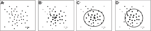
Illustration of the WSVDD model.

Supplementary file 1 provides the proof of (1), where |.|² denotes the L₂–norm of Euclidean space. In order to obtain better data description, the original training data are mapped from the input space into a higher dimensional feature space via a mapping function φ(·). By using the mapping function φ(·), the training data can be more compact and distinguishable in the feature space. The inner product of two vectors in the feature space can be calculated by using the kernel function as $K (x_{i}, x_{j}) = 〈 ϕ (x_{i}), ϕ (x_{j}) 〉$ .²⁶ For class X, the mean of all feature vectors $(1 / N) \sum_{j = 1}^{N} ϕ (x_{j})$ plays the role of the core in the kernel space, which is illustrated in Figure 2B. The weighting w_i, ∀_i = 1,…, N is computed as:

w_{i} = 1 - \frac{d_{i} - \min_{1, \dots, N} {d_{l}}}{\max_{1, \dots, N} {d_{l}} - \min_{1, \dots, N} {d_{l}}}

(2)

The weighting w_i is designed to be inversely proportional to the distance between the corresponding feature and the mean of feature and normalized to the interval [0, 1]. Figure 2B shows the concept of weighting. In this weighting definition, w_i is used to determine the probability that the training data are outliers in the taxonomic class X. In kernel space, the farther away one feature vector φ(x_i) from the core is, the smaller the corresponding weighting w_i is, and the more likely it is that the data point should be taken as an outlier.

Weighted support vector domain description.

To obtain the smallest hyper-sphere that encloses most of the data points in a class X, we need to solve the optimization problem as follows:

\begin{array}{l} \min_{c, r, ξ} r^{2} + C \sum_{i = 1}^{N} w_{i} ξ_{i} \\ s . t . {‖ ϕ (x_{i}) - 0^{*} ‖}^{2} \leq r^{2} + ξ_{i} \\ \forall x_{i} \in X, ξ_{i} \geq 0, i = 1, 2, ...., N \end{array}

(3)

where o^* is center, r is radius, the trade-off parameter C gives the trade-off between the volume of the hyper-sphere and the accuracy of data description, ξ_i ≥ 0 is a slack variable. In equation (3), the smaller the w_i is, the larger the likelihood that the corresponding data point x_i is an outlier. Solving equation (3) (Supplementary file 1 shows how to solve equation (3) in detail.), we obtained the dual problem of (3) as:

\begin{array}{l} \max L = \sum_{i} α_{i} K (x_{i}, x_{i}) - \sum_{i, j} α_{i} α_{j} K (x_{i,} x_{j}) \\ s . t . C w_{i} \geq α_{i} \geq 0, \sum_{i} α_{i} = 1, \forall i \end{array}

(4)

Figure 2C shows the center o^* and some SVs that can be obtained through solving the dual problem. The hyper-sphere S_X(o^*, r), whose contours enclose most of the data points in the kernel space, is defined as: $S_{X} (o^{*}, r) = {x_{i} | {‖ ϕ (x_{i}) - o^{*} ‖}^{2} \leq r^{2}, i = 1, 2, ..., N_{1}}$ , where N₁ is the number of data points inside the hyper-sphere, and N₁ < N. Figure 2D illustrates the hyper-sphere of the class X, where the radius $r = m e a n {‖ ϕ (x_{i}) - o^{*} ‖ | x_{i} \in S V s}$ .

To get the best model, Gaussian kernel function K_G(x_i, x_j) = exp(–(x_i – x_j)² / s²) was used in our experiments. Supplementary file 1 shows how to estimate the most suitable trade-off parameter C and kernel parameter s in detail. The WSVDD's computational complexity analysis and algorithm analysis are also provided in Supplementary file 1.

Decision function

For each inputted testing DNA fragment, we computed its composition vector x. Then we used the following function to decide whether the input vector x belongs to i-th class:

F_{i} (x) = s i g n ({‖ ϕ (x) - o_{i}^{*} ‖}^{2} - r_{i}^{2})

(5)

For all taxonomic classes, if only one F_i(x) < 1 (that is, only one class accepts the inputted vector), then the vector x belongs to the class. If more than two F_i(x) < 1 (that is, more than two classes accept the inputted vector), then the vector x belongs to the min $({‖ ϕ (x) - o_{i}^{*} ‖}^{2} - r_{i}^{2})$ class. If all F_i(x) = 1 (in other words, if all classifiers reject the input vector), then the vector x cannot be classified, and the input vector is defined as unclassified.

Measuring the classification accuracy

To evaluate the performance of the classifier, we computed the sensitivity, specificity, and harmonic mean for each class. These measures have been commonly used to evaluate the performance of methods designed to classify metagenomic fragments,^9–14,19 as they can capture important relationships among the number of true-positive (TP_i), false-positive (FP_i), false-negative (FN_i), and unclassified (U_i) assignments within each taxonomic class i.

The total number of the inputted query DNA fragments from class i can be denoted as: Z_i = TP_i + FN_i + U_i. The sensitivity (Sn_i) is the proportion of the fragments from class i correctly assigned to class i: Sn_i = TP_i / Z_i. The specificity Sp_i is the proportion of the fragments assigned to class i that are correctly assigned: Sp_i = TP_i /(TP_i + FP). Because a robust classifier should have high sensitivity and specificity, we combined sensitivity and specificity in a harmonic mean to evaluate the robustness of class i: (harmonic mean)_i = 2 × Sn_i × Sp_i /(Sn_i + Sp_i).

Here, we report the average of sensitivity, specificity, and harmonic mean over all classes at a respective taxonomic level.

Results

We performed three experiments to evaluate our method. Firstly, we performed experiments to predict the unknown organisms of simulated metagenomes and compared our results with three other methods, PhyloPythiaS,¹⁰ Phymm,¹¹ and TACOA,¹² at the lower taxonomic level. Then, we used WSVDD's training models to analyze the microbial diversity of five real human gut metagenomes. Lastly, we evaluated the effectiveness of outliers on WSVDD and other classifiers. In all experiments, the testing sequences and training sequences were generated by read simulation software MetaSim.²⁷

Training genomes and test genomes

The training genomes and test genomes were downloaded from the US National Center for Biotechnology Information (NCBI) in September 2011. Taxonomic information for each genome was obtained from the NCBI taxonomy database. To evaluate the performance of the classifier, we built a set comprising genomes only from genera represented by at least two distinctly named species. This filtered data set consists of 556 genomes from 297 species, 50 genera. The 50 distinct genera include 45 bacterial genera and 5 archaeal genera. Supplementary file 2 provides some detailed information of the 556 genomes.

Simulated metagenome experiment at the genus and species levels

Because classification at lower taxonomic level is the most difficult task in metagenomic classification, we only performed some experiments to predict the organisms of the simulated metagenomic fragments at the genus and species levels.

In real practice, the taxonomic organism of metagenomic fragments must be predicted when the fragments are from genomes that are not yet represented in the public genome databases. To simulate this, we designed a hold-out experiment to predict the unknown taxonomic organisms of the query DNA fragments. For example, when performing hold-out experiments at the genus (species) level, all training genomes from the species (bacterial strain) being evaluated were removed. However, if the given species (bacterial strain) represented the only species (bacterial strain) within its genus (species), then query fragments from this species (bacterial strain) were removed from the test sets. That is, if a taxonomic organism belongs to the testing sets, then it certainly does not belong to the training sets.

At the genus and species levels, we created three training models using DNA fragments of length 450, 1,000, and 3,000 bp, respectively. Approximately 3,000 randomly sampled DNA fragments were used to train each taxonomic class. More than 150,000 DNA fragments were used to train each model. We also constructed three independent test sets with DNA fragments of length 450, 1,000, and 3,000 bp. The test sets (simulated metagenomes) were constructed by randomly sampling fragments from each genome with the probability of drawing a fragment from a set proportional to its length. The test sets contained 246,519 and 653,319 fragments when performing the hold-out experiment at the genus and species levels, respectively. The results for all different fragment lengths are reported in Figure 3A and B. Supplementary file 3 provides some detailed information of the experimental results.

Figure 3.

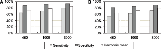
Bars depict the average classification sensitivity, specificity, and harmonic mean for each fragment length at the genus and species levels.

Figure 3A shows that at the genus level, the lengths of the DNA fragments ranged from 450 to 3,000 bp, the sensitivity could be increased from 64.18% to 79.2%, the specificity ranged from 86.17% to 92.76%, and the harmonic mean could be increased from 73.16% to 85.24%. Figure 3B shows, at the species level, that when the lengths of the DNA fragments varied from 450 to 3,000 bp, the sensitivity increased efficiently from 53.9% to 71.58%, the specificity ranged from 79.35% to 87.7%, and the harmonic mean could be increased efficiently from 64.26% to 78.82%.

Comparing Figure 3A with Figure 3B, a general trend was that the average classification of sensitivity, specificity, and harmonic mean at the genus level was higher than that at species level. The sensitivity, specificity, and harmonic mean were improved when classifying longer DNA fragments.

Comparison with other methods on common data set

Here we have compared our identification performance with other three methods, PhyloPythiaS,¹⁰ Phymm,¹¹ and TACOA,¹² on the same test sets (simulated metagenomes) at the genus level. The methods can be used to identify variable-length DNA fragments based on dinucleotide frequency vectors.⁸ PhyloPythiaS¹⁰ is made by SVMs algorithm. Results for PhyloPythiaS were obtained by using the software at http://www.binning.bioinf.mpi-inf.mpg.de/download/.¹⁰ Phymm¹¹ is designed based on the theory of interpolated Markov models. Results for Phymm were obtained by using the software at http://www.cbcb.umd.edu/software/phymm/.¹¹ TACOA¹² is designed by the theory of kernelized-NN. We reprogrammed for TACOA, with the same training genomes and 5-mer frequency vectors. The TACOA's kernel parameters were chosen by cross-validation to yield the optimal specificity over all classes at each taxonomic level.

In order to perform a fair comparison between different methods, we picked out 30 distinct bacterial genera as test sets, because PhyloPythiaS,¹⁰ Phymm,¹¹ and TACOA¹² contained the source genomes of the 30 bacterial genera within their training set. Supplementary file 4 provides some detailed information of the 30 distinct bacterial genera. Then, we constructed three independent test sets by randomly sampling fragments of size 450, 1,000, and 3,000 bp from the 30 bacterial genera. The test set comprised 167,724 fragments. We compared the classification performance by testing the same test sets on PhyloPythiaS,¹⁰ Phymm,¹¹ TACOA,¹² and our WSVDD method. The results obtained from each method are shown in Figure 4 and Supplementary file 4.

Figure 4.

Bars depict the average classification.

WSVDD and Phymm showed higher prediction sensitivities than PhyloPythiaS and TACOA. When the read lengths ranged from 450 to 3,000 bp, the average sensitivity of WSVDD and Phymm increased from 67.02% to 80% and from 59.92% to 78.81%, respectively. At the same time, WSVDD achieved quite competitive average specificity compared with the other three methods. When the read lengths ranged from 450 to 3,000 bp, the average specificity increased from 86.65% to 93.04% for WSVDD, from 64.49% to 79.18% for Phymm, from 86.47% to 95.89% for PhyloPythiaS, and from 92.37% to 97.58% for TACOA.

To estimate robustness, sensitivity and specificity were combined in a harmonic mean. WSVDD achieved the best harmonic mean, which increased from 75.58% to 86.03% when the read lengths increased from 450 to 3,000 bp. PhyloPythiaS and Phymm achieved quite similar harmonic means. The harmonic mean ranged from 65.59% to 83.33% for PhyloPythiaS and from 62.12% to 79% for Phymm. The lowest harmonic mean was produced by TACOA for all variable-length reads. In general, WSVDD has an improved prediction performance.

Application to real metagenomes

To evaluate the performance of WSVDD on real metagenomic data sets, we used WSVDD's training models (1,000 bp, genus level) to analyze the microbial diversity of gut metagenome²⁸ derived from fecal samples of 124 European individuals. Since the data set contains different samples with read lengths varying from 44 to 75 bp, the short Illumina reads have been assembled into longer DNA fragments (~1,600 bp) using the SOAPdenovo tool.²⁹ We downloaded five samples’ reads, from 57 Denmark adults, at http://www.gutmeta.genomics.org.cn/.²⁸ The descriptions of the samples are given in Table 1. The results obtained by WSVDD are shown in Table 2.

Table 1.

Summary of human gut metagenomic data sets.

SAMPLE ID	GENDER	TOTAL LENGTH (Mb)	NO. OF READS	AVERAGE LENGTH OF READS (bp)
MH0001	female	19.69	14,301	1,618
MH0002	female	88.77	65,392	1,680
MH0003	male	119.59	68,658	2,640
MH0004	male	31.92	23,793	1,681
MH0005	male	19.62	14,339	1,684

Table 2.

The results of WSVDD on the real human gut metagenomes.

ABUNDANCE(%)	MH0001	MH0002	MH0003	MH0004	MH0005
Bacteroides	12.92	14.45	15.89	13.94	13.33
Bifidobacterium	4.86	5.78	6.32	5.65	4.81
Clostridium	16.57	16.06	17.15	17.16	16.03
Escherichia	5.3	5.6	5.48	4.87	5.88
Streptococcus	13.03	11.86	13.72	13.03	13.47
Unclassified rate	43.75	41.75	38.51	42.29	43.08
Others	3.57	4.5	2.93	3.06	3.4

At the genus level, WSVDD has identified five main bacterial genera to be differentially abundant: Bacteroides (Bacteroidetes), Bifidobacterium (Actinobacteria), Clostridium (Firmicutes), Escherichia (Proteobacteria), and Streptococcus (Firmicutes) from the human gut metagenomic data set. WSVDD labeled more than 16% of the reads as Clostridium, making it the biggest group, while WSVDD assigned about 13% of the reads to Bacteroides and Streptococcus, making them the second biggest groups. The method also generated different taxonomic distributions of other groups of organisms. For instance, WSVDD assigned about 5% of the reads to Bifidobacterium and Escherichia. As expected, Firmicutes and Bacteroidetes had the highest abundance, about 29% and 14%, respectively.²⁸ About 3% of the reads had been assigned to other genera. The results demonstrate that it is difficult to access the real accuracy, since no reference data set can be obtained for most of the species in the real data set. Therefore, we can see that about 41% of the reads could not be assigned by WSVDD.

The effect of outliers on WSVDD and other classifiers

In practice, each bacterial genome has ~13% abnormal fragments on average, which come from sequencing errors, phage invasions, and some highly expressed genes, etc.^19–22 The abnormal fragments are not expected to be binned correctly with the rest of their host genome, and they can adversely affect the performance of a classifier. To test the gene prediction performance of WSVDD under the outliers, we simulated Sanger reads (1,000 bp) and 454 reads (450 bp) from 30 bacterial genera (Supplementary file 4), respectively.

Every category of read was divided into three subsets. We selected two subsets as the training set, the rest of the subset as the testing set. A percentage of outliers were artificially added to the training sets using read simulation software MetaSim with characteristic noise patterns.²⁷ In the article, the outlier rates were 0%, 1%, 3%, and 10% for Sanger and 454 reads.

After preparing the eight types of training set with different outlier rates, we used the raw test set and the corresponding noisy training set to evaluate WSVDD's performance compared with four other classifiers: SVDD (Support Vector Data Description),^24,30 SVMs,³⁰ Kernelized-NN¹² and SOM.^17,31 The classifiers’ parameters were found by cross-validation to identify the best harmonic mean of each method.³² The results are provided in Figure 5.

Figure 5.

The average sensitivity, specificity, and harmonic mean on.

We can see a decrease of sensitivity, specificity, and harmonic mean for all classifiers on simulated Sanger and 454 reads with increasing outlier rates (Fig. 5). Generally, on Sanger reads, the sensitivity, specificity, and harmonic mean of all methods decrease very slowly (~2%) when the outlier rates increase from 0% to 3%. However, when the outlier rate increases from 3% to 10%, SVDD, Kernelized-NN, SOM, and SVMs decrease drastically in sensitivity (~9%), specificity (~7%), and harmonic mean (~7.8%). WSVDD decreases the most slowly, only 4.3% for sensitivity, 3.8% for specificity, and 3.9% for harmonic mean.

On simulated 454 reads, the sensitivity, specificity, and harmonic mean of all methods decrease faster than Sanger reads for different outlier rates. For SVDD, Kernelized-NN, SOM, and SVMs, drops in sensitivity of ~13.5%, specificity of ~10.6%, and harmonic mean of ~12.5% are observed when the outlier rate increases from 0% to 3%. In reads with an outlier rate of 10%, there is a further decrease in sensitivity of ~15.7%, specificity of ~13%, and harmonic mean of ~14.7% for the methods. Also here, WSVDD showed a smaller decrease, only 4.8% for sensitivity, 4.6% for specificity, and 4.7% for harmonic mean from outlier-free reads to reads with 3% outliers. When the outlier rates increased to 10%, WSVDD showed a decrease in sensitivity of ~7.8%, specificity of ~7%, and harmonic mean of ~7.2%. These results indicate that WSVDD improves the classifier's robustness.

Conclusion and Discussion

In the article, we predict unknown organisms of metagenomic data using WSVDD classifier, which can eliminate the interference from some outliers for the training genomic data and then generate a more accurate data domain description for each taxonomic class. The experimental results demonstrate that the classifier has an improved prediction performance.

There are several opportunities for further development. For one, WSVDD mainly works on DNA fragments with length at least 450 bp, while the current high-throughput sequencing technology produces fragments with lengths varying from 50 bp to 500 bp. Further research is required to combine an effective similarity-based method for assigning short fragments of metagenomic data directly and accurately. In addition, many sequence fragments in a metagenome may originate from species belonging to an entirely new (hitherto unknown) phylum or class. We are planning to develop an algorithm to deduce the appropriate taxonomic level automatically for the new genome fragments.

Author Contributions

Conceived the subject: FL. Designed the experiments, analyzed the data, and wrote the manuscript: TH. Developed the structure and arguments for the paper: YL, QYZ, XZ, KW. All authors reviewed and approved of the final manuscript.

Supplementary Data

Supplementary file 1

The detailed information of WSVDD method.

Supplementary file 2

The detailed information of the downloaded 556 genomes.

Supplementary file 3

The detailed information of the average classification sensitivity, specificity, and harmonic mean for each fragment length at genus and species levels.

Supplementary file 4

The detailed information of the average classification sensitivity, specificity, and harmonic mean for variable fragment length at different methods.

Footnotes

Acknowledgments

The authors thank the associate editor and reviewers for their comments, which were very helpful in improving the manuscript.

References

Turnbaugh

P.J.

, Gordon

J.I.

An invitation to the marriage of metagenomics and metabolomics. Cell. 2008; 134(5): 708–13.

Altschul

S.F.

, Gish

, Miller

, Myers

E.W.

, Lipman

D.J.

Basic local alignment search tool. J Mol Biol. 1990; 215(3): 403–10.

Krause

, Diaz

N.N.

, Goesmann

. Phylogenetic classification of short environmental DNA fragments. Nucleic Acids Res. 2008; 36(7): 2230–9.

Huson

D.H.

, Auch

A.F.

, Qi

, Schuster

S.C.

MEGAN analysis of metagenomic data. Genome Res. 2007; 17(3): 377–86.

Schreiber

, Gumrich

, Daniel

, Meinicke

Treephyler: fast taxonomic profiling of metagenomes. Bioinformatics. 2010; 26(7): 960–1.

Stark

, Berger

S.A.

, Stamatakis

, von Mering

MLTreeMap – accurate maximum likelihood placement of environmental DNA sequences into taxonomic and functional reference phylogenies. BMC Genomics. 2010; 11: 461.

Zhang

, Sun

MetaDomain: a profile HMM-based protein domain classification tool for short sequences. Pac Symp Biocomput. 2012; 17: 271–82.

Campbell

, MRAzek

, Karlin

Genome signature comparisons among prokaryote, plasmid, and mitochondrial DNA. Proc Natl Acad Sci USA. 1999; 96(16): 9184–9.

McHardy

A.C.

, Martin

H.G.

, Tsirigos

, Hugenholtz

, Rigoutsos

Accurate phylogenetic classification of variable-length DNA fragments. Nat Methods. 2006; 4(1): 63–72.

10.

Patil

K.R.

, Haider

, Pope

P.B.

. Taxonomic metagenome sequence assignment with structured output models. Nat Methods. 2011; 8(3): 191–2.

11.

Brady

, Salzberg

S.L.

Phymm and PhymmBL: metagenomic phylogenetic classification with interpolated Markov models. Nat Methods. 2009; 6(9): 673–6.

12.

Diaz

N.N.

, Krause

, Goesmann

, Niehaus

, Nattkemper

T.W.

TACOA – taxonomic classification of environmental genomic fragments using a kernelized nearest neighbor approach. BMC Bioinformatics. 2009; 10(1): 56.

13.

Chan

C.K.

, Hsu

, Halgamuge

, Tang

S.L.

Binning sequences using very sparse labels within a metagenome. BMC Bioinformatics. 2008; 9(1): 215.

14.

Rosen

G.L.

, Reichenberger

E.R.

, Rosenfeld

A.M.

NBC: the Naive Bayes classification tool webserver for taxonomic classification of metagenomic reads. Bioinformatics. 2011; 27(1): 127–9.

15.

Nalbantoglu

O.U.

, Way

S.F.

, Hinrichs

S.H.

, Sayood

RAIphy: phylogenetic classification of metagenomics samples using iterative refinement of relative abundance index profiles. BMC Bioinformatics. 2011; 12(1): 41.

16.

Zhenqiu

, Zhenqiu

, Halima

, Ming

Efficient feature selection and multiclass classification with integrated instance and model based learning. Evol Bioinform. 2012; 8: 197–205.

17.

Weber

, Teeling

, Huang

. Practical application of self-organizing maps to interrelate biodiversity and functional data in NGS-based metagenomics. ISME J. 2010; 5(5): 918–28.

18.

Leung

H.C.

, Yiu

S.M.

, Yang

. A robust and accurate binning algorithm for metagenomic sequences with arbitrary species abundance ratio. Bioinformatics. 2011; 27(11): 1489–95.

19.

Hoff

K.J.

The effect of sequencing errors on metagenomic gene prediction. BMC Genomics. 2009; 10(1): 520.

20.

Trimble

W.L.

, Keegan

K.P.

, D'Souza

. Short-read reading-frame predictors are not created equal: sequence error causes loss of signal. BMC Bioinformatics. 2012; 13: 183.

21.

Zhou

, Olman

, Xu

Barcodes for genomes and applications. BMC Bioinformatics. 2008; 9(1): 546.

22.

Hou

, Liu

, Lin

C.X.

, Li

D.Y.

A new vector for identification of prokaryotes and their variable-size genomes. Curr Microbiol. 2013; 66(1): 96–101.

23.

Wang

C-D

, Lai

Position regularized support vector domain description. Pattern Recognit. 2012; 46: 875–84.

24.

Tax

D.M.

, Duin

R.P.

Support vector data description. Mach Learn. 2004; 54(1): 45–66.

25.

Chor

, Horn

, Goldman

, Levy

, Massingham

Genomic DNA k-mer spectra: models and modalities. Genome Biol. 2009; 10(10): R108.

26.

Hastie

, Tibshirani

, Friedman

, Franklin

The elements of statistical learning: data mining, inference and prediction. Math Intell. 2005; 27(2): 83–5.

27.

Richter

D.C.

, Ott

, Auch

A.F.

, Schmid

, Huson

D.H.

MetaSim – a sequencing simulator for genomics and metagenomics. PLoS One. 2008; 3(10): e3373.

28.

Qin

, Li

, Raes

; MetaHIT Consortium. A human gut microbial gene catalogue established by metagenomic sequencing. Nature. 2010; 464(7285): 59–65.

29.

, Zhu

, Ruan

. De novo assembly of human genomes with massively parallel short read sequencing. Genome Res. 2010; 20(2): 265–72.

30.

Chang

C-C