Sage Journals: Discover world-class research

Abstract

The Prediction of RNA secondary structures has drawn much attention from both biologists and computer scientists. Many useful tools have been developed for this purpose. These tools have their individual strengths and weaknesses. As a result, based on support vector machines (SVM), we propose a tool choice method which integrates three prediction tools: pknotsRG, RNAStructure, and NUPACK. Our method first extracts features from the target RNA sequence, and adopts two information-theoretic feature selection methods for feature ranking. We propose a method to combine feature selection and classifier fusion in an incremental manner. Our test data set contains 720 RNA sequences, where 225 pseudoknotted RNA sequences are obtained from PseudoBase, and 495 nested RNA sequences are obtained from RNA SSTRAND. The method serves as a preprocessing way in analyzing RNA sequences before the RNA secondary structure prediction tools are employed. In addition, the performance of various configurations is subject to statistical tests to examine their significance. The best base-pair accuracy achieved is 75.5%, which is obtained by the proposed incremental method, and is significantly higher than 68.8%, which is associated with the best predictor, pknotsRG.

Keywords

RNA secondary structure support vector machine feature selection statistical test

Introduction

An RNA secondary structure is the fold of a nucleotide sequence. The sequence is folded due to bonds between non-adjacent nucleotides. These bonded nucleotide pairs are called base pairs. Three possible combinations of nucleotides may form a base pair: A-U, G-C, and G-U, where A-U and G-C are called Watson-Crick pairs and G-U is called the Wobble pair. Generally, an RNA secondary structure can be regarded as a sequence S with a set S' of base pairs (i, j), where 1 ≤ i < j ≤ |S| and ∀(i, j), (i', j') ∈ S', i = i' if and only if j = j'. By this definition, no base belongs to more than one base pair. The RNA secondary structure prediction problem is to identify the folding configuration of a given RNA sequence.

There are mainly two kinds of bonded structures, namely nested and pseudoknotted ones. Although prediction techniques on nested structures have been well developed, those on pseudoknotted ones are still limited in accuracy due to high computational requirements.^1,2 A pseudoknotted structure is a configuration in which the bases outside a helix hold hydrogen bonds to form another helix. Given an RNA sequence S with a set S' of base pairs, the sequence is pseudoknotted if in S' there exist two pairs (i, j) and (i', j') such that i < i' < j < j'. These two types of bonded structures are illustrated in Figure 1. In the past decades, lots of tools have been developed to predict the RNA secondary structure. However, for computational reasons, most of them do not take the pseudoknotted structures into considerations as the required computational efforts for some prediction models have been proved to be NP-hard.³

Figure 1.

The nested (top) and pseudoknotted (bottom) bonded RNA structures.

The methods for predicting RNA secondary structures could be roughly categorized into two types, which are based on thermodynamics,^2,4,5 and comparative approaches.^6,7 The thermodynamic approaches manage to integrate some experimentally determined parameters with criteria of minimum free energy. Therefore, the obtained results conform with the true configurations. The comparative approach adopts the sequence comparison strategy. It requires users to input one sequence with unknown structure, and a set of aligned sequences whose secondary structures are known in advance.

For predicting RNA secondary structures, pknotsRG,⁴ RNAStructure,⁸ and NUPACK⁹ are well-developed software tools. Since these tools resort to different criteria, each of them has its own metric and weakness. With their distinctness in prediction power, we propose a tool preference choice method that integrates these softwares in order to improve prediction capability.

Our method is based on the machine learning approach, which includes feature extraction, feature selection, and classifier combination methods. The features are first extracted from the given sequence and then these features are input into the classifier to determine the most suitable prediction software. In this paper, the feature selection methods, mRMR¹⁰ and mRR,¹¹ are employed to identify the important features and SVM (support vector machine)^12,13 is used as the base classifier.

To further improve prediction accuracies, we propose a multi-stage classifier combination method, namely incremental mRMR and mRR. Instead of selecting features independently, our classifier combination method takes the outputs of classifiers in the previous stages into consideration. Thus, the method guides the feature selector to choose the features that are most relevant to the target class label while least dependent on the previously predicted labels. The performance of various combination strategies is further subject to the statistical test in order to examine their significance. The best base-pair accuracy achieved is 75.5%, which is obtained by the proposed incremental mRMR and is significantly higher than 68.8%, the accuracy of the single best prediction software, pknotsRG. The experimental results show that our tool preference choice method can improve base-pair prediction accuracy.

The rest of this paper is organized as follows. In Preliminaries, we will first describe the SVM software and the RNA secondary prediction tools used in this paper. Then, we will present some classifier combination methods. The methods for bootstrap cross-validations are also presented. In addition, we describe features adopted in this paper. The detailed feature extraction methods are presented in Supplementary materials. Feature relevance and feature selection presents the feature relevance and selection. In Classifier combination, we focus on how to integrate multiple classifiers. The data sets used for experiments and the performance measurements are presented in Data sets and performance evaluation. Our experimental results and conclusions are given in Experimental results and conclusions, respectively.

Preliminaries

Support vector machines

Support vector machine (SVM)¹⁴ is a well-established technique for data classification and regression. It maps the training vectors x_i into a higher dimensional space, namely feature space, and finds a separating hyperplane that constitutes the maximal margin in the feature space. The margin is constructed by only a fraction of training data, called support vectors. For subsequent prediction tasks, new data are mapped into that same space and determined which side of the data fall on. To describe the hyperplane in the feature space, the kernel function, K(x_i, x_j) = ϕ(x_i)^Tϕ(x_j), is defined. Among the kernel functions, we adopt radial basis function (RBF),¹⁵ as it yields the best results. In this paper, LIBSVM¹⁵ is used as our SVM classification tool.

pknotsRG

Some algorithms for predicting pseudoknotted structure are based on thermodynamics.^1,5 Since predicting arbitrary pseudoknotted structures in athermodynamic way is NP-complete,¹⁶ Rivas and Eddy² thus took an alternative approach, which is based on the dynamic programming algorithm. Their method mainly focuses on some classes of pseudoknots and the complexity is of O(n⁶) in time and of O(n⁴) in space for the worst case, where n denotes the sequence length. Based on Rivas's system (pknots),² another prediction software tool, pknotsRG,⁴ was developed. The idea is motivated by the fact that H-type pseudoknots are commonly observed in RNA sequences. Hence, by setting some proper constraints, pknotsRG can reduce the required prediction time to O(n⁴) and space to O(n²) for predicting pseudoknotted structures. The program (including source codes and precompiled binary executable codes) is available on the internet for download. Unlike other web-accessible tools, it is free of web service restrictions and it is appropriate for a large amount of data analysis. It folds arbitrary long sequences and reports as many suboptimal solutions as the user requests.

RNAStructure

RNAStructure was developed by Mathews et al,⁸ and it is also based on the dynamic programming algorithm. The software incorporates chemical modification constraints into the dynamic programming algorithm and makes the algorithm minimize free energy. Since both chemical modification constraints and free energy parameters are considered, the software works reasonably better than those that adopt only free energy minimization schemes. The program is also available for both source codes and web services. It can be used for secondary structure and base pair probability predictions. In addition, it also provides a graphical user interface for Microsoft Windows (Microsoft Corporation, Redmond, WA) users.

NUPACK

NUPACK is the abbreviation for Nucleic Acid Package and is developed by Dirks and Pierce.⁹ It presents an alternative structure prediction algorithm which is based on the partition function. Because the partition function gives information about the melting behavior for the secondary structure under the given temperature,¹⁷ the base-pairing probabilities thus can be derived accordingly. The software can be run on the NUPACK webserver. For users who want to conduct a large amount of data analysis, source codes can be downloaded and compiled locally. In most cases, pseudoknots are excluded from the structural prediction.

Majority vote

The majority vote (MAJ)^18,19 assigns an unknown input x to the most representative class according to classifiers' outputs. Suppose that there are m labels and the output of classifier i is represented by an m-dimensional binary vector (d_i,₁, d_i,2, …, d_{i, m}) ∈ {0, 1}^m, 1 ≤ i ≤ L, where d_{i, j} = 1 if x is labeled as class j by the classifier i, otherwise d_{i, j} = 0. The majority vote picks up class c among L classifiers if
$c = a r g \max_{1 \leq j \leq m} \sum_{i = 1}^{L} d_{i, j} .$
(1)

The disadvantage of the original majority vote cannot handle conflicts from classifiers or even numbers. Let us assume that there are four classifiers involved in solving 3-class classification problem. If the outputs of these four classifiers are (1, 0, 0), (0, 1, 0), (1, 0, 0), (0, 1, 0), there would be no way to resolve the conflict. In this paper, we take the idea of weighted majority vote (WMJ), that is, if classifiers' predictions are not equally accurate, then we assign the more competent classifiers more power in making the final decision. Let us take the same problem as an example. If the classification error rates of the four classifiers are 0.1, 0.3, 0.2, and 0.35, respectively, it would be reasonable to report c = 1. This is because the output obtains the most common agreement among all classifiers. Conventionally, the voting weights are expressed in terms of classification error rates. That is, in the weighted majority voting scheme, the voting weight is defined as log((1 - err)/err) x constant,²⁰ where err denotes the error rate and the constant is set to 0.5.

Behavior knowledge space

Behavior knowledge space (BKS)²¹ is a table look-up approach for classifier combinations. Let us consider a classification task for m classes. Assume a classifier ensemble is composed of L classifiers which collaborate to perform the classification task. Given an input x, the ensemble produces a discrete vector E(x) = (d₁, …, d_L) where each d_i, ∈ {1, …, m} represents the output of the ith classifier. Thus, the number of all possible combinations of these L classifiers' outputs is m^L. For the entire training set, the ensemble's outputs constitute a knowledge space, which characterizes these L classifiers' preferences.

In practice, the algorithm can be implemented by a look-up table, called a BKS table. Each entry in the table contains L cells where each cell accumulates the number of the true classes of training samples falling in. During the recognition stage, the ensemble first collects each classifier's output D_i(x), 1 < i ≤ L. Then it locates which entry matches the outputs, and then picks up the class label corresponding to the plurality cell.

Table 1 illustrates an example of the BKS table with m = 3 and L = 2. D₁ and D₂ represent outputs from the two classifiers. Entries below D₁ and D₂ are all possible predictions. Cells below “true class,” which are P₁,P₂, and P₃, are the numbers of class labels that the training data fall into. Thus, each entry in the table contains the most representative label that associates with the preference of the classifier ensemble.

Table 1.
An example of the BKS table

Prediction
True class

D ₁ D ₂ P ₁ P ₂ P ₃

P ₁ P ₁ 10 3 3

P ₁ P ₂ 3 0 6

P ₁ P ₃ 5 4 0

⋮ ⋮ ⋮ ⋮ ⋮

P ₃ P ₂ 2 2 5

P ₃ P ₃ 0 1 6

Adaboost

Adaboost, short for Adaptive Boosting, is a machine learning algorithm,²⁰ which may be composed of any types of classifiers in order to improve performance. The algorithm builds classifiers in an incremental manner. That is, in each stage of single classifier training, the weights of incorrectly classified observations are increased while those of correctly classified observations are decreased. Consequently, subsequent classifiers focus more attention on observations that are incorrectly classified by previous classifiers. Since there are several classifiers involved making decisions, the WMJ approach is adopted. Although the individual classifiers may not be good enough to perform good prediction alone, as long as their prediction power is not random, they would contribute improvements to the final ensemble. In this paper, Adaboost experiments are served as a performance benchmark for classifier combination.

Bootstrap cross-validation

In this paper, we adopt bootstrap cross-validation (BCV)²¹ for performance comparison of classifiers with the k-fold cross-validation. Assume that a sample S = {(x₁, y₁), (x₂, y₂), …, (x_n, y_n)} is composed of n observations, where x_i represents the ith feature vector, whose class label is y_i. A bootstrap sample $S_{b}^{} = {(x_{1}^{}, y_{1}^{}), (x_{2}^{}, y_{2}^{}), \dots, (x_{n}^{}, y_{n}^{})}$ consists of n observations sampled from S with replacement, where 1 ≤ b ≤ B for some B between 50 and 200. For each bootstrap sample $S_{b}^{}$ , a cross-validation is carried out with some learning algorithm. The performance measure c_b, such as error rate, is calculated with $S_{b}^{}$ . The procedure is repeated B times and then the mean performance estimation $C_{B} = \sum_{b = 1}^{B} C_{b} / B$ is evaluated over all B bootstrap samples. Since the distribution of the bootstrap performance measures is approximately normal, the confidence interval and significance level can be estimated accordingly.

Features

The features involved in this paper are summarized in Table 2, and the total number of the features is 742. The last column of the table shows the 50 top-ranking features selected by both mRMR and mRR, which will be discussed later. The hyphen symbol means that no feature of the factor falls into the 50 top-ranking features. All features are detailed in Supplementary materials.

Table 2.
The feature sets and the 50 top-ranking features by mRMR and mRR

ID Feature set Dimension Top ranking feature names, mutual information and standard errors

1 The compositional factor 6 –

2 The bi-transitional factor 18 AC: 0.0163 ± 0.0058; CA: 0.0427 ± 0.0103

3 The distributional factor 20 D_A(3/4): 0.1009 ± 0.0136; D_G(0): 0.0376 ± 0.0084

4 The tri-transitional factor 66 AAC: 0.0289 ± 0.0081; CCA: 0.0162 ± 0.0064 CGA: 0.0229 ± 0.0070; GCA: 0.0195 ± 0.0069 UAG: 0.0127 ± 0.0058; UCG: 0.0063 ± 0.0032

5 The spaced bi-gram factor 18 –

6 The potential base-pairing factor 3 G-C: 0.0225 ± 0.0079

7 The asymmetry of direct-complementary triplets 3 ADCT₁: 0.0380 ± 0.0096

8 The nucleotide proportional factor 12 –

9 The potential single-stranded factor 3 –

10 The sequence specific score 1 The sequence specific score: 0.0089 ± 0.0049

11 The segmental factor 40 Normalized Seg₅: 0.0069 ± 0.0044

12 The sequence moment 15 η₂(C): 0.0142 ± 0.0060

13 The spectral properties 20 P_C: 0.0587 ± 0.0107

14 The wavelet features 20 q₂(A): 0.0191 ± 0.0061, q₂(G): 0.0123 ± 0.0050 q₃(U): 0.0162 ± 0.0056, q₃(ACGU): 0.0198 ± 0.0068

15 The 2D-dynamic representation 19 μ₂₃: 0.0093 ± 0.0034

16 The protein features 375 RF1-P10: 0.0150 ± 0.0059; RF1-V12: 0.0277 ± 0.0082 RF1-Z2: 0.0164 ± 0.0056; RF2–C1 : 0.0138 ± 0.0063 RF2-S12: 0.0179 ± 0.0069; RF2–S5: 0.0135 ± 0.0057 RF2-S8: 0.0317 ± 0.0077; RF2–Z12: 0.0350 ± 0.0095 RF3-C10: 0.0065 ± 0.0037; RF3–H1 : 0.0170 ± 0.0053 RF3-H20: 0.0253 ± 0.0077; RF3-H7: 0.0531 ± 0.0098 RF3-F15: 0.0284 ± 0.0076; RF3–P18: 0.0477 ± 0.0082 RF3-S-14: 0.0329 ± 0.0086; RF3–S7: 0.0275 ± 0.0081 RF3-S9: 0.0174 ± 0.0062; RF3-V12: 0.0396 ± 0.0091 RF3-V16: 0.0121 ± 0.0046

17 The co-occurrence factor 10 –

18 The 2D graphical representation 36 MM-10:0.0023 ±0.0022

19 The dinucleotides factor 32 d₁(C, U): 0.0118 ± 0.0057; d₂(A, G): 0.0078 ± 0.0037 d₂(A, U): 0.0102 ± 0.0050; d₂(C, A): 0.0161 ± 0.0065 d₂(U; G): 0.0203 ± 0.0073

20 The wavelet encoding for 2D graphical representation 24 w₄(ACUG): 0.0189 ± 0.0060; w₃(AGCU): 0.0141 ± 0.0049 w₂(AUCG): 0.0142 ± 0.0055; w₃(AUGC): 0.0111 ± 0.0050

21 The sequence length 1 –

Total 742 50

Feature Relevance and Feature Selection

Feature relevance

In information theory, entropy is a measure of uncertainty of a random variable.²³ The entropy H of a discrete random variable X with possible values x₁, x₂, …, x_h* is formulated as:
$H (X) = - \sum_{i = 1}^{h} p (x_{i}) \log p (x_{i}),$
(2)
where p(x_i) denotes the probability that variable X is of value x_i.

Mutual information I(X, Y) quantifies the dependence between the joint distribution of X and Y, and it is defined as:
$I (X, Y) = H (X) + H (Y) - H (X, Y),$
(3)
where H(X, Y) is the joint entropy of X and Y. If we associate X and Y with the features and class labels, mutual information can be regarded as a relevance measure between these two items. As for the feature selection, mutual information is capable of counting the feature relevance with respect to the class label. The higher the value is, the more relevant a feature is.

Conditional mutual information I(X_i, Y | X_j) stands for how much information variable X_i can explain variable Y, but variable X_j cannot. It is defined as:
$I (X_{i}, Y / X_{j}) = H (X_{i}, Y) + H (X_{j}, Y) - H (X_{i}, Y, X_{j}) - H (X_{j})$
(4)

Assume Y is a dependent variable, and X_i and X_j are independent variables. Conditional mutual information measures the discrepancy of prediction capability between variable X_i and X_j. It can also be considered as a dissimilarity of the two variables in terms of prediction power. In general, the conditional mutual information is not symmetric, that is I(X_i, Y | X_j) ≠ I(X_j, Y | X_i). To account for the distinction between these two variables, the average conditional mutual information D_CMI(X_i, X_j) is usually adopted, that is (I(X_i, Y | X_j) + I(X_j, Y | X_i))/2.

Feature selection

The feature relevance constitutes the basic idea for feature ranking and feature selection. mRMR (minimal redundancy and maximal relevance)¹⁰ and mRR (minimal relevant redundancy)¹¹ are two of well known information theoretic methods.

Most feature selection methods select top-ranking features based on F-score or mutual information without considering relationships among features. mRMR¹⁰ manages to accommodate both feature relevance with respect to class label and dependency among features. The strategy combines both the maximal relevance and the minimal redundancy criteria. The maximal relevance criterion selects feature subset X_r, which contains maximal mutual information with respect to the class label Y.

$m a x D (X_{r}, Y) = \frac{1}{r} \sum_{X_{i \in X r}} I (X_{i}, Y),$
(5)

where X_i is a feature within 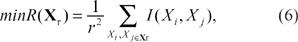X_r and r is the number of selected features contained in X_r. The minimal redundancy criterion imposes mutual dependency constraints between any two selected features as follows:
$m i n R (X_{r}) = \frac{1}{r^{2}} \sum_{X_{i}, X_{j \in X r}} I (X_{i}, X_{j})$
(6)

In order to take the above two criteria into consideration and to avoid an exhaustive search, mRMR adopts an incremental search approach. That is, the rth selected feature should satisfy:
$X_{r} = a r g \max_{X_{j}} {\begin{array}{r} I (X_{j}, Y) - \frac{1}{r - 1} \sum_{X_{i \in X r - 1}} I (X_{j}, X_{i}) | X_{j} \\ \in X - X_{r - 1} \end{array}} \cdot$
(7)

Instead of dealing with dependency between features, mRR¹¹ adopts the conditional mutual information to express distance between features. Let the target number of selected features be denoted by r. The algorithm starts with calculating average conditional mutual information D_CMI(X_i, X_j) between any pair of distinct features. Next, the conditional mutual information is served as distances between features and hierarchical clustering processes are performed repeatedly until r + 1 groups remain. These clusters stands for the most distinct and representative feature groups. Then, the algorithm picks the feature with the highest mutual information from each cluster and sorts them into nonincreasing order. Since the last feature is assumed to come from the feature group of random noises, thus finally, only the first r features are reserved.

Classifier Combination

Incremental feature selection

In this subsection, we propose an incremental feature selection method for improving classification accuracy. Our method is based on the mRMR¹⁰ or mRR¹¹ feature selection method. Our method incrementally selects features in multiple stages. The feature selection in the latter stages involves the factor of the classifier preference of the former stages. Our method has the predicted labels of previous classifiers serve as preselected features, so that the subsequently selected features will be as relevant as possible to the real label, while being the least dependent on these previously predicted labels.

Suppose we take mRMR as our kernel selection function. At stage 1, α features are selected by mRMR and then they are used to train a classifier. In this paper, α is set to 50. Then, the training data elements are predicted by the classifier, and thus the predicted label of each element becomes the output. These predicted labels serve as artificial features for subsequent stages. Consequently, the subsequent feature selection procedure encourages the unselected features, which are most relevant to the real labels, but least dependent on the previously predicted labels. Note that the predicted labels are used only for evaluating the degree of mutual information (conditional mutual information in mRR), but they are not real candidate features to be selected. Since our method is designed to learn incrementally, it is called incremental mRMR (ImRMR). When we invoke mRR as the kernel selection function, our method is called incremental mRR (ImRR).

Our incremental mRMR feature selection method is formally described in Procedure 1. The incremental mRR method is formally given in Procedure 2.

Data Sets and Performance Evaluation

The experimental data sets are obtained from PseudoBase²⁴ and RNA SSTRAND²⁵ websites. We retrieve all PseudoBase and RNA SSTRAND tRNA sequences and their secondary structure information. The sequences are then fed into pknotsRG, RNAStructure, and NUPACK for secondary structure prediction. To determine which software is the most suitable one for a given sequence, we adopt the base-pair accuracy for evaluation.

Suppose we are given an RNA sequence S = a₁a₂ … a_N. Let the real partner of a nucleic base a_i be denoted by $a_{i_{r}}$ where 1 ≤ i ≤ N and 0 ≤ i_r N. If a_i is unpaired, i_r = 0; otherwise, 1 ≤ i_r ≤ N. Let the predicted partner of a_i be $a_{i_{p}}$ . The predicted base-pair accuracy for a single sequence is given by
$Accuracy = 100 % \times \frac{1}{N} \sum_{i = 1}^{N} {\begin{matrix} 1, & if i_{r} = i_{p} \\ 0, & otherwise . \end{matrix}$
(9)

For each sequence, we calculate its base-pair accuracies given by the three softwares and assign a class label, which corresponds to the preferred software to the sequence. The labels are pk, rn, and nu, which are associated with pknotsRG, RNAStructure and NUPACK, respectively. Since our goal is to apply the machine learning approach to identifying the most prominent software for prediction, we remove the sequence that any two softwares have identical highest accuracies in order to avoid ambiguity. Hence, the final numbers are 495 for RNA SSTRAND tRNA and 225 for PseudoBase database. The numbers of the tool preference classes are shown in the first row of Table 3. As we can see, each sequence has its software tool preference for prediction.

Table 3.
Number of sequences and predicted base-pair accuracies in each tool preference class

pk rn nu

Sequences 359 212 149 Total = 720

BP accuracy 68.80% 64.55% 60.92% Extreme = 79.20%

The second row of Table 3 shows the overall base-pair accuracy, which each software alone predicts all sequences; it also shows the extreme level of accuracy that arises when we select the correct software for predicting each sequence. In the table, BP means base-pair. The overall accuracy here is defined as the quotient of the total number of correctly predicted bases and total number of bases from all sequences. It implied that we can obtain a more powerful predictor if the preference classification task is done well.

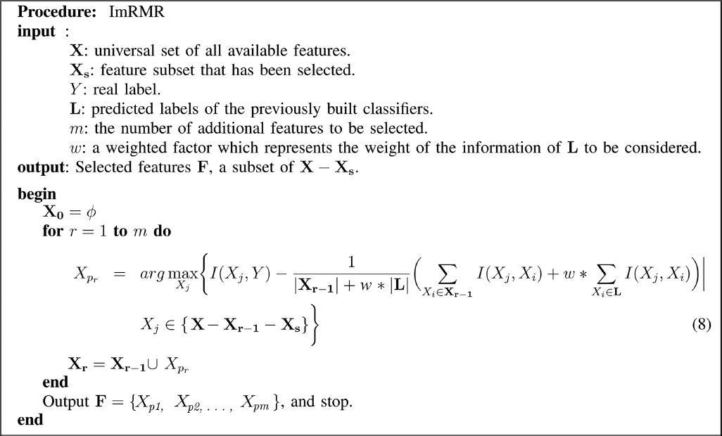
Procedure 1.

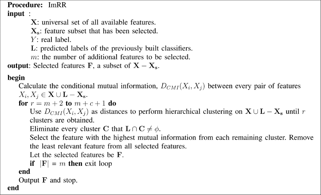
Procedure 2.

We adopt two performance measures for comparison, the classification accuracy and base-pair accuracy. The classification accuracy here is defined as Q = Σp_i/N, where p_i denotes the number of testing targets; those belong to class i and are correctly classified, and N denotes the total number of testing targets.

Experimental Results

We first perform classification experiments and then compare their performance. In each experiment, the leave-one-out cross-validation (LOOCV) method is used in order to obtain the average performance measure. Since our main goal is to obtain a tool selector with a good base-pair accuracy. Hence, for the base-pair accuracy, the BCV is first carried out and significant tests are conducted. Finally, we perform feature analysis and identify important features.

Experiments for classification accuracy

By default, mRMR selects the 50 most prominent features, and we also adopt this setting for mRR. Hence, at each stage, we obtain 50 features to train classifiers. The original feature selection of each stage in mRMR or mRR does not consider the classifiers' predicted labels from the previous stages. Thus, in our ImRMR or ImRR, once features are selected, we just exclude them and perform the original mRMR or mRR procedure in the subsequent stages.

The methods for classifier fusion include weighted majority vote (WMJ) and behavior knowledge space (BKS). Table 4 shows the experimental result of various combinations. Since there are two kernel feature selection methods mRMR and mRR, and two classifier fusion methods BKS and WMJ, four totally different combinations are obtained. In each combination, two feature selection configurations, the original (or non-incremental) and our incremental, are compared. The weighted factor w for ImRMR is set to 1. In the table, 1 + … + C, where 1 ≤ C ≤ 4, means the classifiers built in stages from 1 to C are combined together. The last row of this table shows the performance of Adaboost, which will be discussed later.

Table 4.
Classification accuracies of various fusion configurations

1 1 + 2 1 + 2 + 3 1 + 2 + 3 + 4

BKS

a. mRMR 68.3 69.7 (+1.4) 71.0 (+1.3) 72.4 (+1.4)

b. ImRMR 68.3 71.8 (+3.5) 73.4 (+1.6) 74.0 (+0.6)

c. mRR 68.1 69.2 (+1.1) 70.3 (+1.1) 70.0 (−0.3)

d. ImRR 68.1 71.1 (+3.0) 73.1 (+2.0) 74.4 (+1.3)

WMJ

e. mRMR 68.3 68.8 (+0.5) 68.2 (−0.6) 67.8 (−0.4)

f. ImRMR 68.3 69.3 (+1.0) 69.6 (+0.3) 70.2 (+0.6)

g. mRR 68.1 68.3 (+0.2) 67.2 (−1.1) 66.9 (−0.3)

h. ImRR 68.1 68.5 (+0.4) 69.2 (+0.7) 69.6 (+0.4)

Adaboost

200 features from b. 69.2 71.3 (+2.1) 72.8 (+1.5) 72.8 (+0.0)

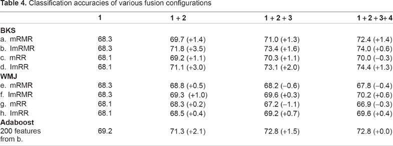
It is observed that the classification accuracies of the incremental feature selection (ImRMR or ImRR) are higher than those of the original one. This may be due to the fact that the additional discriminant information is involved. Comparing results obtained from BKS and WMJ configurations, b, d, f, and h, we can see that BKS achieves higher accuracies. This is because WMJ can not reach correct answers when most classifiers give wrong predictions. In contrast, BKS can deal with the dilemma because it records data that are consistently misclassified (and classified) by classifiers and thus corrects the final answers. It is interesting to note that configuration g achieves the worst result. This may be due to the fact that the acquired feature subsets in each stage are extracted from the almost identically corresponding clusters as the previous stages; nearly no extra information is obtained.

During the fourth stage of BKS fusion, there should be 3⁴ = 81 distinct patterns of classifier preferences. However, we find that less than 81 patterns are formed occasionally, and thus we have to trace back to the BKS table of the third stage. In addition, if we proceed the same procedure to the fifth stage, which will have at most 3⁵ = 243 distinct patterns, we would get a BKS table that is quite sparse. Since we only have 719 samples for building BKS tables, it would imply that the fusion results may not be reliable enough. In this sense, the diversity or the sparseness of BKS tables would implicitly limit the times of fusion. As a result, only four stages were performed.

For the configurations e and g, after the third stage, the classification accuracies keep going down. This is because the most prominent features have been selected in the previous stages; the classifiers built in the subsequent stages would get less competent. Once the system starts to be dominated by these incompetent classifiers, the classification accuracies would go down. However, compared with configuration f and h, it again shows the merit of the incremental feature selection strategy.

To understand how the data fusion has effect on the classification accuracies, all 742 features and 200 features of configurations a, b, c and d (from Table 4) are used for LOOCV experiments, which are made without combining classifiers. The experiments about 200 features of configurations e, f, g, and h are omitted because of similar settings. The results are shown in Table 5. It reveals that training with all 742 features deteriorates the classification as too many incompetent features would ruin the system. Compared with configuration b and d in Table 4, it shows that the systems built with BKS or WMJ fusion achieve higher classification accuracies. This is because each group of 50 selected features is specialized for both the class label and the classifier preference of the previous stages. The obtained improvement exists only when the above condition is satisfied. Once these features are combined directly, conflicts may occur among these features. Consequently, the classification accuracies are not so good.

Table 5.
The classification accuracies of combined features

Feature configurations Percentage

a (200) 68.1

b (200) 69.2

c (200) 68.3

d (200) 68.9

742 66.3

The last row in Table 4 shows the performance of Adaboost, whose base classifier is SVM and the number of stages is also set to four to comply with the previous experiments. To avoid randomness, we use the sample weights to derive exact sample numbers for training. That is, at each stage, the normalized sample weights are first multiplied by the number of total training samples and then rounded to integers. Samples are trained with their individual rounded numbers. Since the standard SVM does not perform feature selection, the best 200 features of configuration b is adopted throughout the experiments.

With the similar weighted majority vote for fusion, it shows that the Adaboost ensemble outperforms those of configurations/and h. This may be due to the fact that the Adaboost ensemble always uses good feature subset for classification while those of configuration f and h adopt less and less dominant features gradually. Hence, even being able to provide distinct information, the base classifiers of configuration f and h are not so competent. When comparing performances of the Adaboost ensemble and that of configuration a, the former one only yields a slightly better classification rate. Since the mRMR ranks features according to both maximal relevance and minimal redundancy, the base classifier in each stage is intrinsically distinct. In addition, the BKS mechanism also facilitates recording the preference of base classifiers. Even still, when compared with the Adaboost ensemble, the configuration a does not explicitly enhance the training of not-yet-learned samples. This may partly account for its lower accuracy. However, when we compare the configuration a and b, the latter one more explicitly focuses on information that has theoretically not been learned. Hence, the classification accuracies get elevated again. For the adaptation to what has not been learned yet, the Adaboost algorithm is more aggressive than information-theoretical methods because it directly aims at wrongly classified samples. Nevertheless, by choosing the classifier combination method to appropriately accommodate the classifier preference, as shown in configuration a, the comparative performance is still possible to be achieved.

Significance test for the base-pair accuracy and feature analysis

In this paper, we adopt bootstrap cross-validation²² to verify which configuration is statistically significant in base-pair accuracy. The accuracies of each configuration are obtained by applying B = 50 bootstrap sampling procedures and then performing LOOCV (k = 720). The overall procedure is shown as follows. Procedure 3, the configuration H_j represents any one from Tables 4 and 5.

Before performing statistical tests, base-pair accuracies of each configuration are subject to the Kolmogorov-Smirno test²⁶ to ensure normality. Following Table 4, to examine whether incremental approaches are significantly better than non-incremental ones in base-pair accuracy, we extracted A_bj from the above procedure, where j can be any configuration from Tables 4 and 5. Since the distribution of the bootstrap performance measures is approximately normal, we perform a paired t-test.²⁷ Table 6 shows the P-values for incremental against non-incremental ones for mRMR and mRR combined with BKS or WMJ fusion. The P-value is the probability of obtaining a test statistic to reject the null hypothesis, which means that there exists no systematic difference in base-pair accuracy between incremental against non-incremental fusions. The smaller the P-value, the stronger the test rejects the null hypothesis. It shows that there is merely 10% ((0.11 + 0.09 + 0.08 + 0.09)/4) that incremental approaches are not significantly better than non-incremental ones on average. In other words, there is a large probability that incremental approaches are significantly better than non-incremental ones. Consequently, we will not include non-incremental fusion approaches further in the subsequent comparison.

Table 6.
Paired t-test of base-pair accuracies for incremental versus non-incremental ones for BKS or WMJ fusion

Configurations BKS WMJ

ImRMR vs. mRMR 0.11 0.09

ImRR vs. mRR 0.08 0.09

Table 7 shows the classification, base-pair prediction accuracies, and numbers of selected features under various configurations. Each value behind the base-pair accuracy is the percentage exceeding the baseline accuracy, which is achieved by the most prominent software, pknotsRG. As the table shows, applying all features for prediction tool choice achieves 72.2% base-pair accuracy, which is higher than the baseline accuracy. If the feature selection methods, such as mRMR and mRR, are adopted, the accuracies can be improved. Furthermore, once the incremental feature selection methods are combined with their tailored fusion methods, the results are further improved. The best base-pair accuracy achieved is 75.5%.

procedure 3.

Table 7.
The classification and base-pair prediction accuracies of various configurations

Configuration Features (#) Classification accuracy (%) Base-pair accuracy (%)

pknotsRG – – 68.8

All features 742 66.3 72.2 (+3.4)

mRMR 50 68.3 72.9 (+4.1)

mRR 50 68.1 72.5 (+3.7)

Adaboost 200 72.8 73.8 (+5.0)

ImRMR + WMJ 50 × 4 70.2 73.0 (+4.2)

ImRR + WMJ 50 × 4 69.6 73.2 (+4.4)

ImRMR + BKS 50 × 4 74.0 75.5 (+6.7)

ImRR + BKS 50 × 4 74.4 75.2 (+6.4)

To verify the significance in base-pair prediction capability in Table 7, we first apply both normality tests and analysis of variance (ANOVA) analysis to ensure the obtained performance measures are adequate for the subsequent statistical tests.²⁸ Since there indeed exists difference, we thus conduct the TukeyHSD test²⁷ for further examination. Table 8 illustrates the P-values obtained from the TukeyHSD test in a pairwise manner. Each P-value[i, j] represents the significance for the ith row item against the corresponding jth column. The symbols ‘(++)’ and ‘(+)’ indicate 95% and 90% significance levels, respectively. For example, P-value [i = 2,j = 1] indicates that the SVM tool selector, trained with the features selected by mRMR, significantly outperforms pknotsRG in base-pair accuracy. However, P-value [i = 2,j = 2] implies that the mRMR-SVM selector is almost of the same power as the SVM selector with all features. As the table shows, all selectors have significantly higher base-pair accuracy than pknotsRG. The first three selectors (all features, 50 mRMR features, and 50 mRR features) are equally well tool selectors. This further implies that both mRMR and mRR are powerful feature selection methods and the prediction capability with 50 features is good enough to compete that with all features. The composite selectors (from row four to row eight) are dominantly better than any single selector. Except for ImRMR + WMJ, it is difficult to distinguish which composite selector is significantly powerful. It may imply that the proposed incremental fusion approach is comparable to Adaboost, even with fewer features in each fusion stage. In addition, it seems that the BKS and WMJ fusions are not significantly different.

Table 8.
TukeyHSD test for base-pair accuracies

pknotsRG All features mRMR mRR ImRMR + WMJ ImRR + WMJ Adaboost ImRMR + BKS

All features 0.000 (++)

mRMR 0.000 (++) 1.000

mRR 0.000 (++) 1.000 1.000

ImRMR + WMJ 0.000 (++) 0.000 (++) 0.000 (++) 0.000 (++)

ImRR + WMJ 0.000 (++) 0.000 (++) 0.000 (++) 0.000 (++) 1.000

Adaboost 0.000 (++) 0.000 (++) 0.000 (++) 0.000 (++) 0.976 0.999

ImRrMRr + BKS 0.000 (++) 0.000 (++) 0.000 (++) 0.000 (++) 0.140 0.353 0.776

ImRRrr + BKS 0.000 (++) 0.000 (++) 0.000 (++) 0.000 (++) 0.055 (+) 0.175 0.545 1.000

The last column in Table 2 shows the 50 top-ranking features selected by both mRMR and mRR, which may represent the most important features for the SVM-based tool choice. The 50 features are obtained as follows. We start from m = 50, which represents top-ranking features by both mRMR and mRR. Then we check whether the intersection of the two selected feature sets is of size 50. If the size is not equal to 50, we set m = m + 1 and repeat the above procedure until 50 intersected features are selected. Following each feature in the table, the estimated mutual information and standard error are calculated.²⁹ We find that these features indeed come from diverse sources. Among those, there are 19 protein features, and 13 features come from the bi-transitional, tri-transitional, and dinucleotide factors. Other feature factors, like the compositional, spaced bi-gram, nucleotide proportional, potential single-stranded, co-occurrence, and length ones, are not included. These factors can be regarded as less prominent feature sets for the purpose of tool choice, since mutual information is a relevance measure between feature and label. From the ratio of the mutual information to standard error, we can conjecture how accurate the relevance is. If we use 2.0 as a ratio threshold, there are only four features, MM-10, Seg₅, RF3-C10, and the sequence specific score, whose ratios are below this threshold, and those associated with the rest of 46 features are above the threshold. Hence, the obtained relevance information can be considered reliable. It is worth mentioning that the length feature is categorized as less important. It thus implies that our SVM-based tool selector relies little on the sequence length information. Consequently, this method may be extended to other RNA sequences, like truncated ones, without sacrificing too much accuracy.

Conclusions

In this paper, we propose a tool preference choice method, which can be used for RNA secondary structure prediction. Our method is based on the machine learning approach. That is, the preferred tool can be determined by more than one classifier. The tool choice starts by extracting features from the RNA sequences. Then the features are inputted into the classifier or ensemble to find out the most suitable tool for prediction. We apply the feature selection methods to identify the most discriminant features. Although these methods are proven to be powerful, they still require users to specify the number of features to be picked up. Hence, we adopt the default settings and devise data fusion methods tailored to the feature selection. The classifiers are thus trained with selected features incrementally. The number of combinations (ensembles) is determined implicitly by the fusion methods, which could be the diversity of classifiers' predicted labels or cross-validation accuracies. The experiments reveal that our tool choice method for the RNA secondary structure prediction works reasonably well, especially combined with the feature selection method and some fusion strategies. The best achieved base-pair accuracy is 75.5%, which is significantly higher than those of any stand-alone prediction software. Note that up to now, pknots RG is the best predictor, which has an accuracy rate of 68.8%.

Although we use RNA sequences from two databases and adopt three prediction softwares in this paper, our method is flexible for adding new features, RNA sequences, or new prediction software tools in the future. To further improve the prediction accuracies, more features could be exploited in the future. For example, researchers proposed other 2D,^30–34 3D,^35–39 4D,⁴⁰ 5D,⁴¹ and 6D⁴² graphical representations for discrimination of nucleotide sequences. These features are able to differentiate sequences of real species and may also be useful for the tool choice purpose.

Prediction	True class
P ₁	P ₁	10	3	3
P ₁	P ₂	3	0	6
P ₁	P ₃	5	4	0
⋮	⋮	⋮	⋮	⋮
P ₃	P ₂	2	2	5
P ₃	P ₃	0	1	6

ID	Feature set	Dimension	Top ranking feature names, mutual information and standard errors
1	The compositional factor	6	–
2	The bi-transitional factor	18	AC: 0.0163 ± 0.0058; CA: 0.0427 ± 0.0103
3	The distributional factor	20	D_A(3/4): 0.1009 ± 0.0136; D_G(0): 0.0376 ± 0.0084
4	The tri-transitional factor	66	AAC: 0.0289 ± 0.0081; CCA: 0.0162 ± 0.0064 CGA: 0.0229 ± 0.0070; GCA: 0.0195 ± 0.0069 UAG: 0.0127 ± 0.0058; UCG: 0.0063 ± 0.0032
5	The spaced bi-gram factor	18	–
6	The potential base-pairing factor	3	G-C: 0.0225 ± 0.0079
7	The asymmetry of direct-complementary triplets	3	ADCT₁: 0.0380 ± 0.0096
8	The nucleotide proportional factor	12	–
9	The potential single-stranded factor	3	–
10	The sequence specific score	1	The sequence specific score: 0.0089 ± 0.0049
11	The segmental factor	40	Normalized Seg₅: 0.0069 ± 0.0044
12	The sequence moment	15	η₂(C): 0.0142 ± 0.0060
13	The spectral properties	20	P_C: 0.0587 ± 0.0107
14	The wavelet features	20	q₂(A): 0.0191 ± 0.0061, q₂(G): 0.0123 ± 0.0050 q₃(U): 0.0162 ± 0.0056, q₃(ACGU): 0.0198 ± 0.0068
15	The 2D-dynamic representation	19	μ₂₃: 0.0093 ± 0.0034
16	The protein features	375	RF1-P10: 0.0150 ± 0.0059; RF1-V12: 0.0277 ± 0.0082 RF1-Z2: 0.0164 ± 0.0056; RF2–C1 : 0.0138 ± 0.0063 RF2-S12: 0.0179 ± 0.0069; RF2–S5: 0.0135 ± 0.0057 RF2-S8: 0.0317 ± 0.0077; RF2–Z12: 0.0350 ± 0.0095 RF3-C10: 0.0065 ± 0.0037; RF3–H1 : 0.0170 ± 0.0053 RF3-H20: 0.0253 ± 0.0077; RF3-H7: 0.0531 ± 0.0098 RF3-F15: 0.0284 ± 0.0076; RF3–P18: 0.0477 ± 0.0082 RF3-S-14: 0.0329 ± 0.0086; RF3–S7: 0.0275 ± 0.0081 RF3-S9: 0.0174 ± 0.0062; RF3-V12: 0.0396 ± 0.0091 RF3-V16: 0.0121 ± 0.0046
17	The co-occurrence factor	10	–
18	The 2D graphical representation	36	MM-10:0.0023 ±0.0022
19	The dinucleotides factor	32	d₁(C, U): 0.0118 ± 0.0057; d₂(A, G): 0.0078 ± 0.0037 d₂(A, U): 0.0102 ± 0.0050; d₂(C, A): 0.0161 ± 0.0065 d₂(U; G): 0.0203 ± 0.0073
20	The wavelet encoding for 2D graphical representation	24	w₄(ACUG): 0.0189 ± 0.0060; w₃(AGCU): 0.0141 ± 0.0049 w₂(AUCG): 0.0142 ± 0.0055; w₃(AUGC): 0.0111 ± 0.0050
21	The sequence length	1	–
	Total	742	50

	pk	rn	nu
Sequences	359	212	149	Total = 720
BP accuracy	68.80%	64.55%	60.92%	Extreme = 79.20%

	1	1 + 2	1 + 2 + 3	1 + 2 + 3 + 4
BKS
a. mRMR	68.3	69.7 (+1.4)	71.0 (+1.3)	72.4 (+1.4)
b. ImRMR	68.3	71.8 (+3.5)	73.4 (+1.6)	74.0 (+0.6)
c. mRR	68.1	69.2 (+1.1)	70.3 (+1.1)	70.0 (−0.3)
d. ImRR	68.1	71.1 (+3.0)	73.1 (+2.0)	74.4 (+1.3)
WMJ
e. mRMR	68.3	68.8 (+0.5)	68.2 (−0.6)	67.8 (−0.4)
f. ImRMR	68.3	69.3 (+1.0)	69.6 (+0.3)	70.2 (+0.6)
g. mRR	68.1	68.3 (+0.2)	67.2 (−1.1)	66.9 (−0.3)
h. ImRR	68.1	68.5 (+0.4)	69.2 (+0.7)	69.6 (+0.4)
Adaboost
200 features from b.	69.2	71.3 (+2.1)	72.8 (+1.5)	72.8 (+0.0)

Feature configurations	Percentage
a (200)	68.1
b (200)	69.2
c (200)	68.3
d (200)	68.9
742	66.3

Configurations	BKS	WMJ
ImRMR vs. mRMR	0.11	0.09
ImRR vs. mRR	0.08	0.09

Configuration	Features (#)	Classification accuracy (%)	Base-pair accuracy (%)
pknotsRG	–	–	68.8
All features	742	66.3	72.2 (+3.4)
mRMR	50	68.3	72.9 (+4.1)
mRR	50	68.1	72.5 (+3.7)
Adaboost	200	72.8	73.8 (+5.0)
ImRMR + WMJ	50 × 4	70.2	73.0 (+4.2)
ImRR + WMJ	50 × 4	69.6	73.2 (+4.4)
ImRMR + BKS	50 × 4	74.0	75.5 (+6.7)
ImRR + BKS	50 × 4	74.4	75.2 (+6.4)

	All features	mRMR	mRR	ImRMR + WMJ	ImRR + WMJ	Adaboost	ImRMR + BKS
All features
mRMR	1.000
mRR	1.000	1.000
ImRMR + WMJ	0.000 (++)	0.000 (++)	0.000 (++)
ImRR + WMJ	0.000 (++)	0.000 (++)	0.000 (++)	1.000
Adaboost	0.000 (++)	0.000 (++)	0.000 (++)	0.976	0.999
ImRrMRr + BKS	0.000 (++)	0.000 (++)	0.000 (++)	0.140	0.353	0.776
ImRRrr + BKS	0.000 (++)	0.000 (++)	0.000 (++)	0.055 (+)	0.175	0.545	1.000

Footnotes

Author Contributions

Conceived and designed the experiments: CBY, CYH. Analysed the data: CYH, CHC. Wrote the first draft of the manuscript: CYH, CHC, CTT. Contributed to the writing of the manuscript: CYH, CBY, HHC. Agree with manuscript results and conclusions: CYH, CBY. Jointly developed the structure and arguments for the paper: CYH, CBY, HHC. Made critical revisions and approved final version: CBY. All authors reviewed and approved the final manuscript.

Funding

This research work was partially supported by the National Science Council of Taiwan under contract NSC-98-2221-E-110-062.

Competing Interests

Author(s) disclose no potential conflicts of interest.

Disclosures and Ethics

As a requirement of publication author(s) have provided to the publisher signed confirmation of compliance with legal and ethical obligations including but not limited to the following: authorship and contributorship, conflicts of interest, privacy and confidentiality and (where applicable) protection of human and animal research subjects. The authors have read and confirmed their agreement with the ICMJE authorship and conflict of interest criteria. The authors have also confirmed that this article is unique and not under consideration or published in any other publication, and that they have permission from rights holders to reproduce any copyrighted material. Any disclosures are made in this section. The external blind peer reviewers report no conflicts of interest.

Supplementary Materials

We describe the feature extraction used in this paper.

References

Matsui

, Sato

, Sakakibara

Pair stochastic tree adjoining grammars for aligning and predicting pseudoknot RNA structures. Bioinformatics. 2005; 21(11): 2611–7.

Rivas

, Eddy

S.R.

A dynamic programming algorithm for RNA structure prediction including pseudoknots. J Mol Biol. 1999; 285(5): 2053–68.

Lyngsø

R.B.

, Pedersen

C.N.S.

Pseudoknots in RNA secondary structures. Res Comput Mol Biol. 2000; 201–9.

Reeder

, Steffen

, Giegerich

pknotsRG: RNA pseudoknot folding including near-optimal structures and sliding windows. Nucleic Acids Res. 2007; 35(Web Server issue): W320–4.

Zuker

Mfold web server for nucleic acid folding and hybridization prediction. Nucleic Acids Res. 2003; 31(13): 3406–15.

Cai

, Malmberg

R.L.

, Wu

Stochastic modeling of RNA pseudoknotted structures: a grammatical approach. Bioinformatics. 2003; 19 Suppl 1: i66–73.

Tahi

, Engelen

, Regnier

A fast algorithm for RNA secondary structure prediction including pseudoknots. Proceedings of the Third IEEE Symposium on Bioinformatics and Bioengineering. Bethesda, MD, USA; 2003.

Mathews

D.H.

, Disney

M.D.

, Childs

J.L.

, Schroeder

S.J.

, Zuker

, Turner

D.H.

Incorporating chemical modification constraints into a dynamic programming algorithm for prediction of RNA secondary structure. Proc Natl Acad Sci USA. 2004; 101(19): 7287–92.

Dirks

R.M.

, Pierce

N.A.

An algorithm for computing nucleic acid base-pairing probabilities including pseudoknots. J Comput Chem. 2004; 25(10): 1295–304.

10.

Peng

, Long

, Ding

Feature selection based on mutual information: criteria of max dependency, max-relevance, and min-redundance. IEEE Transaction on Pattern Analysis and Machine Intelligence. 2005; 27(8): 1226–38.

11.

Sotoca

J.M.

, Pla

Supervised feature selection by clustering using conditional mutual information-based distances. Pattern Recognit. 2010; 43(6): 2068–81.

12.

Ben-Hur

, Horn

, Siegelmann

H.T.

, Vapnik

Support vector clustering. J Mach Learn Res. 2001; 2: 125–37.

13.

Cortes

, Vapnik

Support-vector networks. Machine Learning. 1995; 20(3): 273–97.

14.

Vapnik

The Nature of Statistical Learning Theory. Berlin: Springer-Verlag; 1995.

15.

Chang

C.C.

, Lin

C.J.

LIBSVM: a library for support vector machines [homepage on the Internet]. Taiwan: National Science Council of Taiwan. Available from: http://www.csie.ntu.edu.tw/~cjlin/libsvm. Accessed.

16.

Reeder

, Giegerich

Design, implementation and evaluation of a practical pseudoknot folding algorithm based on thermodynamics. BMC Bioinformatics. 2004; 5: 104.

17.

McCaskill

J.S.

The equilibrium partition function and base pair binding probabilities for RNA secondary structure. Biopolymers. 1990; 29(6–7): 1105–19.

18.

Ruta

, Gabrys

A theoretical analysis of the limits of majority voting errors for multiple classifier systems. Pattern Anal Appl. 2002; 5(4): 333–50.

19.

Kuncheva

L.I.

, Whitaker

C.J.

Measures of diversity in classifier ensembles and their relationship with the ensemble accuracy. Machine Learning. 2003; 51(2): 181–207.

20.

Kuncheva

L.I.

“Fuzzy” versus “nonfuzzy” in combining classifiers designed by boosting. IEEE Transactions on Fuzzy Systems. 2003; 11(6): 729–41.

21.

Raudys

, Roli

The behavior knowledge space fusion method: analysis of generalization error and strategies for performance improvement. Proceedings of the International Workshop on Multiple Classifier Systems (LNCS 2709). Springer; 2003: 55–64.

22.

W.J.

, Carroll

R.G.

, Wang

Estimating misclassification error with small samples via bootstrap cross-validation. Bioinformatics. 2005; 21(9): 1979–86.

23.

MacKay

D.J.C.

Information Theory, Inference and Learning Algorithms. Cambridge: Cambridge University Press; 2003.

24.

van Batenburg

F.H.

, Gultyaev

A.P.

, Pleij

C.W.

PseudoBase: structural information on RNA pseudoknots. Nucleic Acids Res. 2001; 21(9): 194–5.

25.

Andronescu

, Bereg

, Hoos

H.H.

, Codon

RNA STRAND: the RNA secondary structure and statistical analysis database. BMC Bioinformatics. 2008; 9: 340.

26.

Zar

J.H.

Biostatistical Analysis, 5th ed. Engelwood Cliffs, NJ: Prentice-Hall, Inc; 2009.

27.

R Development Core Team. R: A Language and Environment for Statistical Computing. Vienna: R Foundation for Statistical Computing; 2008.

28.

Demšar

Statistical comparisons of classifiers over multiple data sets. J Mach Learn Res. 2006; 7: 1–30.

29.

Moddemeijer

On estimation of entropy and mutual information of continuous distributions. Signal Processing. 1989; 16: 233–48.

30.

Guo

, Randic

, Basak

S.C.

A novel 2-D graphical representation of DNA sequences of low degeneracy. Chem Phys Lett. 2001; 350(1–2): 106–12.

31.

Huang

, Liao

, Li

, Liu

H-L curve: a novel 2D graphical representation for DNA sequences. Chem Phys Lett. 2008; 462(1–3): 129–32.

32.

Liu

X.Q.

, Dai

, Xiu

, Wang

PNN-curve: a new 2D graphical representation of DNA sequences and its application. J Theor Biol. 2006; 243(4): 555–61.

33.

Randic

Graphical representations of DNA as 2-D map. Chem Phys Lett. 2004; 386(4–6): 468–71.

34.

Song

, Tang

A new 2-D graphical representation of DNA sequences and their numerical characterization. J Biochem Biophys Methods. 2005; 63(3): 228–39.

35.

Cao

, Liao

, Li

A group of 3D graphical representation of DNA sequences based on dual nucleotides. International Journal of Quantum Chemistry. 2008; 108: 1485–1490.

36.

Liao

, Wang

T.M.

3-D graphical representation of DNA sequences and their numerical characterization. J Mol Struct. 2004; 681(1–3): 209–12.

37.

Z.H.

, Fan

T.R.

PN-curve: a 3D graphical representation of DNA sequences and their numerical characterization. Chem Phys Lett. 2007; 442(4–6): 434–40.

38.

X.Q.

, Wen

, Qi

Z.H.

New 3D graphical representation of DNA sequence based on dual nucleotides. J Theor Biol. 2007; 249(4): 681–90.

39.

, Sun

, Wang

J.H.

TN curve: a novel 3D graphical representation of DNA sequence based on trinucleotides and its applications. J Theor Biol. 2009; 261(3): 459–68.

40.

Chi

, Ding

Novel 4D numerical representation of DNA sequences. Chem Phys Lett. 2005; 407: 63–7.

41.

Liao

, Li

, Zhu

, Xiang

On the similarity of DNA primary sequences based on 5-D representation. J Math Chem. 2007; 42(1): 47–57.

42.

Liao

, Wang

T.M.

Analysis of similarity/dissimilarity of DNA sequences based on nonoverlapping triplets of nucleotide bases. J Chem Inf Comput Sci. 2004; 44(5): 1666–70.

43.

Huang

C.D.

, Lin

C.T.

, Pal

N.R.

Hierarchical learning architecture with automatic feature selection for multiclass protein fold classification. IEEE Trans Nanobioscience. 2003; 2(4): 221–32.

44.

Wang

, Zhang

Characterization and similarity analysis of DNA sequences based on mutually direct-complementary triplets. Chem Phys Lett. 2006; 426(4–6): 324–8.

45.

M.K.

Visual pattern recognition by moment invariants. IRE Transactions on Information Theory. 1962; 8(2): 179–87.

46.

Percival

D.B.

, Walden

A.T.

Wavelet Methods for Time Series Analysis (Cambridge Series in Statistical and Probabilistic Mathematics). New York: Cambridge University Press; 2000.

47.

Gupta

, Mittal

, Singh

A time-series-based feature extraction approach for prediction of protein structural class. EURASIP J Bioinform Syst Biol. 2008; 235451.

48.

Bielinska-Waz

, Clark

, Waz

, Nowak

, Nandy

2D-dynamic representation of DNA sequences. Chem Phys Lett. 2007; 442: 140–4.

49.

Bielinska-Waz

, Nowak

, Waz

, Nandy

, Clark

Distribution moments of 2D-graphs as descriptors of DNA sequences. Chem Phys Lett. 2007; 443: 408–13.

50.

Nirenberg

, Leder

, Bernfeld

. RNA codewords and protein synthesis, VII. On the general nature of the RNA code. Proc Natl Acad Sci USA. 1965; 53(5): 1161–8.

51.

Ding

C.H.

, Dubhack

Multi-class protein fold recognition using support vector machines and neural networks. Bioinformatics. 2001; 17(4): 349–58.

52.

Leydesdorff

, Vaughan

Co-occurrence matrices and their applications in information science: extending ACA to the web environment. Journal of the American Society for Information Science and Technology. 2006; 57(12): 1616–28.

53.

Randić

, Marjan

, Lerš

, Plavšić

Novel 2-D graphical representation of DNA sequences and their numerical characterization. Chem Phys Lett. 2003; 368: 1–6.

54.

Randić

, Vračko

, Lerš

, Plavšić

Analysis of similarity/dissimilarity of DNA sequences based on novel 2-D graphical representation. Chem Phys Lett. 2003; 371: 202–7.

Prediction		True class
D ₁	D ₂	P ₁	P ₂	P ₃
P ₁	P ₁	10	3	3
P ₁	P ₂	3	0	6
P ₁	P ₃	5	4	0
⋮	⋮	⋮	⋮	⋮
P ₃	P ₂	2	2	5
P ₃	P ₃	0	1	6

A Tool Preference Choice Method for RNA Secondary Structure Prediction by SVM with Statistical Tests

Abstract

Keywords

Introduction

Preliminaries

Support vector machines

pknotsRG

RNAStructure

NUPACK

Majority vote

Behavior knowledge space

Adaboost

Bootstrap cross-validation

Features

Feature Relevance and Feature Selection

Feature relevance

Feature selection

Classifier Combination

Incremental feature selection

Data Sets and Performance Evaluation

Experimental Results

Experiments for classification accuracy

Significance test for the base-pair accuracy and feature analysis

Conclusions

Footnotes

Author Contributions

Funding

Competing Interests

Disclosures and Ethics

Supplementary Materials

References