Sage Journals: Discover world-class research

Abstract

Influenza is a highly contagious disease that causes seasonal epidemics with significant morbidity and mortality. The ability to predict influenza peak several weeks in advance would allow for timely preventive public health planning and interventions to be used to mitigate these outbreaks. Because influenza may also impact the operational readiness of active duty personnel, the US military places a high priority on surveillance and preparedness for seasonal outbreaks. A method for creating models for predicting peak influenza visits per total health-care visits (ie, activity) weeks in advance has been developed using advanced data mining techniques on disparate epidemiological and environmental data. The model results are presented and compared with those of other popular data mining classifiers. By rigorously testing the model on data not used in its development, it is shown that this technique can predict the week of highest influenza activity for a specific region with overall better accuracy than other methods examined in this article.

Keywords

influenza prediction association rule mining fuzzy logic predictor variables

Introduction

Influenza is a highly contagious acute febrile disease caused by a single-stranded RNA orthomyxovirus transmitted by airborne respiratory droplets and aerosols, as well as direct contact.¹ While many influenza viruses infect humans, some only infect certain animal species (eg, chickens, ducks, and swine). However, even these viruses have the potential to develop the ability to infect humans. The genetic material of the virus is organized into eight segments of negativesense RNA. New strains of the virus can rapidly emerge via antigenic shift or the re-assortment of these different RNA segments when a cell becomes infected by more than one strain. New influenza strains also develop via antigenic drift of their surface proteins, allowing the virus to evade the host immune response.² Therefore, new influenza vaccines are developed each year to keep up with newly emerging strains of the virus.³

Influenza typically presents with sudden onset of fever of 37.8 C or greater, along with a cough, pharyngitis, rhinorrhea, myalgia, headache, and fatigue. In the pediatric population, symptoms may also include vomiting and diarrhea.⁴ Although the disease is commonly self-limiting, it can progress to influenza pneumonia, which has a significant mortality.⁵ Influenza-associated deaths in USA have been estimated to be less than 0.4 per 100,000 persons per year in general but can be as high as 17 deaths per 100,000 persons per year in those over 65 years of age.⁶ Taubenberger and Morens reviewed influenza pandemics since the year 1500 and noted that influenza pandemics often result in greater-than-expected mortality even among those without comorbid conditions.⁷ The 2009 influenza outbreak illustrated the rapidity with which a new strain can develop into a pandemic and the limitations of available rapid point-of-care testing to detect the outbreak.⁸ Because influenza causes significant morbidity, can be fatal, and often presents with new strains, the prediction of influenza outbreaks in advance can be of value in allowing for timely preventive public health planning and interventions to be used to mitigate the effect of these outbreaks, particularly when outbreaks may be large enough to challenge or overwhelm medical treatment facilities.

The US military places a high priority on surveillance and preparedness for seasonal influenza because it may impair the operational effectiveness of active duty personnel and cause morbidity and mortality among the broader US Department of Defense (DoD) health-care beneficiary population. While immunization against seasonal strains is required for active duty personnel, military units may still experience significant influenza outbreaks,⁹ and recruits may acquire infection early in training, before vaccine-induced immunity develops.¹⁰ Across the global Military Health System, which provides care for active duty personnel as well as family members and retirees, influenza-like illness (ILI) dynamics mirror those of civilian populations in their regions.¹¹

Nsoesie et al¹² published a systematic review of influenza prediction models in 2013. They found that there were significant differences in measures used to assess accuracy of these models, making it difficult to compare them. Many of these models were based on retrospective determination of statistically significant correlation coefficients, which more accurately measure data trends instead of how close a prediction is to the observations.¹² Another difficulty with comparing the models was the variability in how far in the future the predictions were made. For example, one model might have better performance than another but only predict one to two weeks in advance instead of five to six weeks in advance. Models also differed in exactly what they predicted, such as outbreak onset versus outbreak peak. Some models used analysis of web-based query trends, although the Web reports of possible influenza activity that often means an outbreak has already begun; thus, the model is more of an early detector than a predictor of outbreak onset. Such models may still be useful in predicting the outbreak peaks, although Nsoesie et al¹² noted that such web-based estimates might distort the accuracy of the predicted outcomes.

Near the end of 2013, Shaman et al¹³ published a method for predicting the peak weeks of seasonal influenza using ensembles of susceptible–infected–recovered–susceptible models that included adjusting for absolute humidity conditions. These models were trained using a metric that the authors referred to as ILI+, which they defined as a product of the weekly Google Flu Trends estimate with a weekly estimate (obtained from laboratory data) of the percentage of patients presenting with ILI who actually have influenza. Predictions of peak seasonal influenza were considered to be accurate if they were within plus or minus one week of the observed ILI+ peak. Also, starting from the beginning of the season, the model predicted the week number of the (single) peak for the entire season and updated the prediction each week. As a result, some of the predictions were very far in the future (>10 weeks), and many were actually in the past. The reported accuracy varied a great deal among jurisdictions but appeared to be good overall.

In 2014, Chretien et al¹⁴ published a review that was not meant to be systematic but was scoping in order to characterize the prediction methodologies and identify research gaps. They found that there was an apparent acceleration in the number of influenza prediction articles in recent years. These articles described diverse prediction model approaches ranging from purely statistical to mechanistic epidemiological modeling. Consistent with the results of Nsoesie et al,¹² Chretien et al¹⁴ recommended that future prediction studies should provide a consistent and realistic measure of accuracy so that they might be more indicative of real-time prediction.

The purpose of this study is to use the US military ILI data to predict the week of peak ILI visits per total health-care visits. The US Centers for Disease Control and Prevention (CDC) specifies that the case definition of ILI is a fever greater than or equal to 37.8 C, plus a cough and/or sore throat, in the absence of a known cause other than influenza.¹⁵ The influenza outbreak prediction method presented herein was developed by beginning with techniques for creating models that were successful in previous studies for dengue^16,17 and malaria outbreak predictions¹⁸ but are now adapted to influenza. These techniques include data mining from disparate data sets (such as meteorological, climatological, socioeconomic, and influenza case data), the use of an automatic fuzzy association rule model builder, and the objective evaluation of the resulting classifiers to determine a final influenza prediction model. This data-driven approach takes into account the very complex interrelationships that may exist among the disparate variables. By keeping separate the data used in model development from that used for testing, a much less biased estimate of prediction accuracy is provided. This approach helps to avoid accuracy assessments complicated by model overfitting.¹⁹ To provide a model that is operationally useful, our approach takes into account the fact that all data are not always immediately available on the date of collection. Finally, this approach involves criteria derived from the intended user in order to provide a timely advance notice of an influenza outbreak for a region while minimizing false positives (FPs), which may result in alarm fatigue and unnecessary preparation of limited resources, and false negatives (FNs), which may lead the users to question whether the predictive capability is adding value.

Materials and Methods

Extract–transform–load refers to a process in database usage, especially in data warehousing that involves extracting (downloading) data from outside sources, transforming (or normalizing) the data to fit operational needs, and loading the data into the end database or operational store.²⁰ In the context of our prediction methodology, the raw predictor-variable data are downloaded, transformed to work with the prediction model, and loaded into a geospatially enabled database for easy retrieval by the model. The raw data are referenced by jurisdictional division and mapped to geographical resolution. The data are also selected and arranged with respect to both geographic and temporal resolution for exporting to the model.

Predictor variables and their preprocessing

Military influenza case data

The US Armed Forces Health Surveillance Center provided health data as two large files. One of these contained each military health-care visit designated as ILI, as defined earlier, and included fields for date, military treatment facility (MTF), cohort (service member or other health-care beneficiary), age group, and sex. The other file was designated summary data and included these same fields for all military health-care visits. We define ILI activity as ILI visits divided by total visits, by date. While this ratio is often called incidence in the literature, it may not strictly be incidence because the available data did not distinguish new cases from repeat cases, and because the total visits do not necessarily reflect the number of people in the population at risk for the disease. In this article, it is assumed that the ILI activity defined above is a proxy for incidence. The weeks designated in the MTF data often, but not always, coincided with CDC's epidemiological weeks. CDC's epidemiological weeks are numbered from the beginning of the calendar year with weekly intervals beginning on Sundays.¹⁵ Converting to CDC's epidemiological weeks was necessary because this was the convention used for all data in the data mining methods.

In order to obtain US state-level aggregation, the data were first parsed into MTF-level files. The ILI time series and summary time series were then extracted for each MTF. The ILI time series were created by accumulating patients for each date according to CDC's epidemiological weeks. Using a military-designated list of active MTFs and the US states in which they were located, all MTFs in each state were aggregated to obtain state-level data.

Preanalysis of the data included scrutinizing the data for anomalies, possible nonstationarity, and changes in the collection and reporting over the duration of the data. These data were analyzed first at the county level for all counties in the National Capital Region, which includes the District of Columbia and surrounding counties in Maryland and Virginia. Data were then analyzed at the state level for all US states, the District of Columbia, and territories of Guam, the Virgin Islands, and Puerto Rico.

Because the goal of the analysis was to calculate the week of peak ILI activity, several methods for automatically calculating the peaks in historical data were devised. These methods were evaluated, and the most precise method was chosen to identify peaks in the formatted data. Discussion of the peak algorithms appears in the “Methodology” section.

Preanalysis of the data uncovered a change in the character of the data in nearly all the MTFs after mid-2006. The anomaly is illustrated via the aggregated data for Maryland as shown in Figure 1. In this figure, we see that the normalized totals for ILI rise slightly after mid-2006, but the total visits jump very abruptly after mid-2006. This reflects increased access to health-care encounter data beginning at that time and yielded lower ILI activity due to the increased number of summary visits (denominator used in ILI activity). Therefore, we excluded data prior to August 2006 from this study. In contrast to this 2006 anomaly, a smaller ILI data increase occurred in 2012 in the Maryland data. However, no known external factors could be associated with it so it was possibly a real data change. It did not seem to impact the overall ILI data, so we did not exclude these data.

Figure 1

Illustration of data anomaly prior to mid-2006. The normalized ILI cases and the normalized total cases are plotted versus time for all military treatment facilities in Maryland. The ILI cases rise slightly after mid-2006, but the total cases jump sharply after mid-2006.

US CDC's influenza data

In addition to the US military ILI activity described earlier, the following additional predictor variables were obtained from the US CDC's Weekly Influenza Surveillance Reports.²¹ Data from 2006 to present were preprocessed to get one weekly value per jurisdiction.

•

Weekly percentage of patient visits to US health-care providers for ILI, weighted on the basis of state population. These rates are provided for 10 regions in USA. Each US state within a region was assigned the value for that region.

•

Weekly percentage of influenza tests positive for all types of influenza, as reported by laboratories located in all 50 states, Puerto Rico, and the District of Columbia. These rates are provided for 10 regions in USA. Each US state within a region was assigned the value for that region.

•

Weekly percentage of all deaths reported through the 122 Cities Mortality Reporting System that had pneumonia and influenza reported as the underlying or contributing cause of death on the death certificate. These data were provided for nine regions in USA. Each US state within a region was assigned the value for that region.

•

Weekly reports of laboratory-confirmed influenza-associated hospitalizations per 100,000 population in children and adults are monitored through the Influenza Hospitalization Surveillance Network. Each US state within a region was assigned the value for that region.

Environmental data

Previous studies have found that certain environmental variables appear to be related to influenza incidence. A recent review²² described studies characterizing relationships between influenza cases and precipitation, humidity, and temperature. Therefore, based on the environmental variables reported in the literature, the data decribed below were examined for use as predictor variables for influenza. For the following, data from 2006 to present were preprocessed to obtain one weekly value per jurisdiction.

Weather station measurement data were obtained from the US National Climate Data Center.²³ Appropriate weather stations were manually identified for each of the states. These data were not used as predictor variables per se but were used to derive the relative and specific humidity values described below: weekly maximum and mean air temperature and weekly maximum and mean atmospheric pressure. The following is a list of the predictor variables that were based upon the weather station data:

•

Weekly maximum and mean dew point temperatures. The dew point temperature is one type of measurement of atmospheric water vapor and is the temperature below which this water vapor will condense into liquid and at the same rate evaporate at constant atmospheric pressure. The dew point temperature data were obtained directly from the weather station measurements.

•

Weekly maximum and mean relative humidity values. Relative humidity is the percentage or ratio of the partial pressure of water vapor in humid air to the saturation vapor pressure over a flat surface of water at the same temperature. Because saturation vapor pressure is a function of temperature, relative humidity therefore depends upon temperature as well as water vapor content. The relative humidity was calculated from the temperature, pressure, and dew point data.²⁴

•

Weekly mean and maximum specific humidity values. Specific humidity is the ratio of the mass of water vapor to the total mass of a parcel of moist air. The specific humidity was calculated from the temperature, pressure, and dew point data.²⁴

The following satellite-based measurements were used as predictor variables:

•

Rainfall–-weekly mean rainfall amounts were derived from satellite measurements of three-hour rainfall amounts.²⁵ For each state, the values that fall within its borders are summed and then converted from rainfall rate to rainfall amounts by aggregating a week's worth of these data.

•

Land surface temperature–-weekly mean land surface temperatures were derived from daily land surface temperature data measured by satellite.²⁶ These daily data included both day and night temperatures, which were aggregated by week to obtain a mean weekly value.

Methodology

Peak identification

Because the task associated with this analysis is the prediction of influenza peaks, historic peaks need to be identified. The definition of peak is somewhat ambiguous in this context. Weekly data aggregation and noise yield a nonsmooth time series, even when the data are aggregated by week (Fig. 2). The first large oscillation on the left exhibits two possible peaks. Other large oscillations typically exhibit a noncentral peak. Another possible ill-defined issue is when a yearly period contains more than one peak. In order to resolve these issues in an automated fashion (ie, to make the definition of a peak consistent throughout the identification process), we developed four automated peak-finding objective-based algorithms and then chose the one that consistently identified a subjective definition of peak. Having a consistent definition of ILI peak is important for evaluating the prediction accuracy.

The automated peak identification method relies on the definition of a candidate peak as a local maximum, that is, as a time series value that has a positive (discrete) derivative on the left and a negative derivative on the right. As illustrated in Figure 2, there are typically many such local maxima, which make peak identification difficult. The peak-finding algorithm must screen these peak candidates using statistical criteria that do not require human re-identification.

Figure 2

Notional example of peak identification, illustrating why influenza peak identification can be difficult. The highest points of each year should be the peaks, but some years exhibit multiple peaks. The question marks indicate those points that do not exhibit maximum activity for the year but arguably could be considered as peaks.

Various candidate algorithms using both the running average of the time series (at each point, the algorithm calculates the average and standard deviation of all values up to and including that point) and the local average of the time series (at each point, the algorithm calculates the average and standard deviation of the 25 weeks previous to the value, the value itself, and 24 weeks after the value, with adjustments on either end of the time series). These two averaging methods, respectively, insure that peak averages are larger than other local maxima and that peak selection responds to variation in the flu season from year-to-year.

We ran comparisons of four candidate algorithms on selected state-level aggregate data (Fig. 3) and determined that our Method 3 most consistently identified one peak per year, identified what appeared to be the highest peak in a year, and did not identify many spurious peaks. These criteria were consistently fulfilled by Method 3 across all states. Therefore, Method 3 algorithm was chosen for automated peak identification on all state data.

Figure 3

Peak identification for Maine, using four different methods. The red asterisks are the peaks identified by each method.

Method 3 identifies the peak candidates using the discrete derivative criterion (positive derivative immediately prior to the candidate and negative derivative for the time immediately following the peak) and then calculates the running mean and standard deviation of both the data and the discrete derivatives of the data at every point. A candidate peak is chosen as a peak if the following criteria are met:

•

The candidate peak's data value is higher than the running average + two times the running standard deviation AND.

•

The absolute value of the candidate peak's pre- and postderivatives is higher in magnitude than the average + one standard deviation of the respective pre-and postderivatives.

If there are more than 10 peaks identified over the entire time series, peaks are retained only if they are the maximum peak in a 20-week window centered at the peak. The criteria for deciding peaks were chosen to be objective measures for which there are some statistical and geometric bases. Two standard deviations away from the mean are typically considered outliers, so this was the basic criterion using several different ways to smooth the data and account for local fluctuations. The discrete pre- and postderivative conditions describe a peak geometrically: cases before the peak should rise and cases after the peak should fall. The ability to identify multiple peaks per year was necessary but carefully screened by looking for the highest value in the local window. None of the criteria alone could identify what a human would consider the yearly peak, but together the criteria approximated the judgment that a human observer would use to identify one or more yearly peaks. Moreover, the automated criteria were chosen to be defensible (in terms of the definition of peak) and consistent even with fluctuating data.

Final peak algorithm

Although Method 3 was relatively consistent in mathematical terms, its definition of a peak was still unclear. Based on telephone conversations with personnel from the CDC's Influenza Division, the final step of peak identification was performed manually on the results of Method 3. Figure 4 shows an example of final peak identification. Peaks around weeks 100, 185, 205, 255, and 310 were designated as spurious and removed. Peaks around weeks 155, 280, and 284 were added. When a candidate peak's value was within 5% of the value of the highest peak for a given season, it was included. This rationale is to compensate for possible reporting problems. In some cases, it is difficult to identify one true peak in a season. For example, in Figure 4, peaks at 280, 284, and 286 are all certainly reasonable candidates. Method 3 alone successfully identified 87.4% of the 421 true peaks in the data. The use of the automated algorithm together with clearly defined manual rules insured that peak identifications for ground truth purposes were consistent. The above-described method consistently identified at least one peak per year and in some cases more than one peak per year.

Figure 4

Final peak designation for Alaska ILI activity, after manual intervention.

Steps in the prediction method

Prediction models are created using data mining from a large number of data sources by following these steps:

Identification of predictor variables: predictor variables are identified by a manual literature review for articles that report significant correlations of the given disease incidence with environmental and socioeconomic variables. These data are downloaded from available sources. These variables were described in the “Predictor Variables and Their Preprocessing” section.

Model builder: this is the principal part of the method where all the data mining elements reside. After preprocessing, the data are used to find fuzzy association rules. A subset of these rules that satisfy certain criteria is then selected to create a classifier that becomes the prediction model. The data mining elements are detailed as follows:

Data preprocessing and fuzzification: preprocessing is performed to convert the predictor variables into the desired spatiotemporal resolution, as described in detail in Buczak et al.¹⁶ For these predictor data, the spatial resolution is one state, and the temporal resolution is one week. Using the fuzzy set theory,²⁷ these training data are then transformed into membership values (ie, fuzzified).

Rule extraction using fuzzy association rule mining (FARM): FARM,²⁸ a set of data mining methods that use a fuzzy extension of the Apriori algorithm,²⁹ is used to automatically extract the so-called fuzzy association rules from the training data. Fuzzy association rules are of the following form:

IF (X is A) - > (Y is B)

where X and Y are variables, and A and B are membership functions that characterize X and Y, respectively. X is called an antecedent, and Y is called a consequent of the fuzzy association rule. An example of a fuzzy association rule (not used in influenza prediction) is

IF (Rainfall is LARGE) and (Temperature is HOT) - > (Humidity is HIGH)

This rule uses the linguistic term (fuzzy set) HOT for temperature. In this example, the fuzzy set HOT assigns temperatures of 70°F, 80°F, and 100°F to have a degree of membership of 0.1, 0.8, and 1, respectively. Note that fuzzy association rules use linguistic terms (eg, LARGE, HOT, and HIGH) so they are easily understood by humans.

Rule selection using specific metrics: the prediction model is based upon a classifier, which is a set of rules. After the new data are downloaded and preprocessed, all the rules that match the antecedent of the rule are executed. The average of consequents constitutes the prediction for the given data point. The final classifier is selected based on a set of predetermined criteria, and this classifier constitutes the prediction model. Therefore, it is necessary to determine which of the thousands of rules automatically extracted by FARM should be used. A small subset of rules is automatically chosen to minimize the misclassification error on the fine-tuning data set. These choices are made using selection criteria based upon the following three most important metrics for association rules: confidence, lift, and support.

Confidence may be considered as the conditional probability that, if the antecedents are true, then the consequent is true. A rule with confidence of 1 is always true. Support is a measure of how general a given rule might be in the data. Support may be considered as the probability of occurrence of records with given antecedents and consequents in a particular data set. A support of 0.01 means that a given rule describes 1% of a particular data set. Lift indicates the extent to which the antecedents and consequents are not independent. The higher the lift, the more dependent the variables are. A thorough description of these rule metrics and associated equations can be found in Buczak et al¹⁶ and Kuok et al.²⁸

Two approaches for building the classifier were developed and are called One-Classifier 1 and One-Classifier 2. One-Classifier 1 is based on extensions of the method of Liu et al,³⁰ as described in Buczak et al,¹⁶ and orders all the rules first by confidence, next by lift, and finally by the number of antecedents. One-Classifier 2 is based on extensions of the method of Liu et al,³⁰ as described in Buczak et al,¹⁸ and orders all the rules by the pessimistic error rate of Quinlan.³¹ This ranking was developed to better handle noisy data sets. Both methods were tried so that this expectation could be verified.

Finally, a grid search is performed to select optimal misclassification weights for each class by comparing performance on the fine-tuning data set. By optimizing the misclassification weights, a much higher weight may be selected for misclassifying the cases with a small number of exemplars than for those with a large number of exemplars. The ILI dataset contained fewer peaks relative to nonpeaks, so it was important to account for this imbalance to enable the classifier to accurately classify the peaks. This weighting of the misclassification errors during the training step forces the classifier to learn to predict the rare class accurately (even if this causes the unweighted overall accuracy to go down). As mentioned earlier, the selected classifier becomes the prediction model, which is used in Step 3.

Prediction generator: using the prediction model created in Step 2, the prediction generator periodically computes predictions. This is done weekly as new input data become available because the temporal resolution is one week. It should be emphasized that this model uses only data that would actually be available on the date when the prediction was generated. For example, say we want to do a prediction now (week T) and temperature data are available only for week T-2 because of latency in data availability for downloading. The model would not attempt to use data for week T-1 because it is not available. However, the model can still produce a prediction even without the unavailable data. Once these data become available, they automatically undergo preprocessing and are fed into the prediction model that computes predictions, which are then displayed on a map. The outcome variable is peak present/not present in four to six weeks.

Metrics used for model evaluation

The following four performance metrics were used and are defined later: true positive (TP), true negative (TN), FP, and FN.

•

Positive predictive value (PPV): the proportion of positive ILI peak predictions that are real peaks, given by $PPV = \frac{TP}{TP + FP}$ .

•

Negative predictive value (NPV): the proportion of negative peak (ie, no peak) predictions that are not peaks, given by $NPV = \frac{TN}{TN + FN}$ .

•

Sensitivity: the proportion of correctly predicted ILI peaks (also called the probability of detection), given by $sensitivity = \frac{TP}{TP + FN}$ .

•

Specificity: the proportion of correctly predicted non-peaks (1 – specificity equals the false alarm rate), given by $specificity = \frac{TN}{TN + FP}$ .

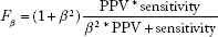
The importance of each of these metrics may vary with how the model is used in practice. One consideration is whether the user considers it more important for the model output to have a high PPV or a high sensitivity. A high PPV indicates that, when the model predicts an ILI peak for a particular week at a particular location, such a peak is very likely to actually occur. When disease prevention and mitigation resources are limited, public health departments consider it very important to have a high PPV in order to mitigate the effects of ILI peaks and thereby reduce morbidity and mortality. Having a high PPV and a low sensitivity means that, when a peak is predicted, the probability is high that it will occur, but only a small percentage of actual peaks are predicted. Therefore, the models were also evaluated using the F score,³² which is derived from the PPV and sensitivity metrics described earlier:

F_{β} = (1 + β^{2}) \frac{PPV * sensitivity}{β^{2} * PPV + sensitivity}

When β equals one, PPV and sensitivity are weighted equally. Assigning β a value less/greater than one gives more importance to PPV/sensitivity. Therefore, β values of 0.5 and 3 were used to give more importance to PPV and sensitivity, respectively. This was done because the public health practitioners whom we consulted thought that both sensitivity and PPV were important but could not agree on which was more important. The performance of the models with the best F_0.5 and F₃ values is presented in this article.

Results

The original data set consisted of ILI case data from the MTFs across all 50 states and 4 US territories during the period from December 2000 through April 2013. These data were aggregated both geographically and temporally to obtain weekly military ILI counts for each state and territory. All the data were combined geographically such that any regional correlation effects were ignored for this study. As mentioned earlier, an anomaly was discovered during analysis that necessitated the removal of all data prior to the 2006-2007 flu season from the study. In addition, because the time series were incomplete for two of the states (North Dakota and Vermont) and all four territories, these were excluded from the study.

For model development and testing, the data from the 48 remaining states were divided into training, fine-tuning, and testing sets. The training set covered August 27, 2006, to July 31, 2011. The fine-tuning set covered August 1, 2010, to July 31, 2011. The testing data set covered August 7, 2011, to January 6, 2013. Note that there were 117 true peaks in the testing data set. The results are always reported only on testing data, as these data were not seen by the model during development.

For the predictor variables, time lags of 1–12 weeks (ie, time stamps T-1, …, T-12) were used as inputs to the model builder. For some of these variables (eg, temperature), the data most recently available at the time of prediction are from time T-2 instead of T-1, so only data from T-2 to T-12 were used.

It is worth noting here that there is a difference in the nomenclature for how many weeks ahead the prediction is made between what is used in this study and what is sometimes used in the literature.¹³ In actual practice, there is almost always a lag between when data are collected and when they are available. In the literature, the counting of the number of weeks ahead often starts from the last date on which the data were collected even if the actual prediction was made later because the data were not immediately available. While this may be a legitimate way to count, it can be confusing to endusers and result in accuracy values better than that expected in actual practice. To provide accuracy measures closer to those expected in operational use, this study defines the count as starting from when the data would actually be available and the prediction could be made, which is assumed to be one week after it is collected. Therefore, when we describe a four-to six-week ahead prediction window, this is actually five to seven weeks removed from the last date on which any data used to make the prediction were collected.

Two different approaches for building the classifiers have been developed. The first approach is a fusion approach in which three separate classifiers are built and their results fused; the second approach consists of training a single classifier. In the fusion approach, we built the following three separate classifiers: one for predicting a peak at T + 4, one for T + 5, and one for T + 6. The outputs of the classifiers were fused by an OR statement:

If (Predicted_Peak_T + 4 OR Predicted_Peak_T + 5 OR Predicted_Peak_T + 6) then Predicted_Peak 4_6.

Therefore, if any one of these three classifiers predicts a peak, then the fusion result is a peak predicted sometime during weeks 4–6 from the date of prediction. Note that the fusion approach only predicts whether there is an ILI peak during weeks 4–6 without identifying which one of these weeks might occur. A TP would then be an actual ILI peak occurring any time during weeks 4–6 when the fusion model predicts a peak. The results for the fusion approach are shown in Table 1.

Table 1

Performance of different prediction methods on test data set.

METHOD	PPV	NPV	SENSITIVITY	SPECIFICITY	F _0.5	F ₃
Fusion of three classifiers	0.379	0.935	0.622	0.842	0.411	0.585
One-Classifier 1	0.509	0.990	0.698	0.977	0.538	0.672
One-Classifier 2	0.603	0.987	0.613	0.986	0.605	0.612

Note: The best value of each performance metric is underlined.

The three separate classifiers use the same input data but produce different results for desired output. The classifier predicting a peak at T + 4 uses a set of rules to produce the desired output peak information at T + 4 weeks; similarly, for the one for predicting a peak at T + 5, it uses a set of rules to produce the desired output peak information at T + 5 weeks, and so on. This means that different rules will be extracted for predicting T + 4, T + 5, or T + 6, leading to classifiers with different rules.

In the second approach, a single classifier is trained that produces peak prediction windows of three weeks in length. These windows are predicted four weeks in advance (ie, they cover weeks T + 4 through T + 6). For this approach, any actual peak that occurred within one of the predicted windows was counted as a TP and any that did not were counted as FN. Any predicted window that did not coincide with an actual peak was counted as a FP, and all other weeks were TN. This is equivalent to predicting a peak five weeks in advance and counting predictions that are accurate within one week of the actual peak, as was done by Shaman et al.¹³ Two such classifiers were trained, and their metrics are shown as One-Classifier 1 and One-Classifier 2 in Table 1. Recall that One-Classifier 1 uses the rule ranking from Buczak et al,¹⁶ while One-Classifier 2 uses the pessimistic error rate of Quinlan.³¹ Figures 5–7 show some examples of the actual peaks and the prediction windows from the second of these classifiers. Figure 5 shows the results for Hawaii where there are 2 TPs, 1 FP, and 72 TNs. Figure 6 shows the results for Wisconsin where there are 2 TPs and 73 TNs. Figure 7 shows the results for Mississippi where there are 2 TPs, 1 FN, and 72 TNs.

Figure 5

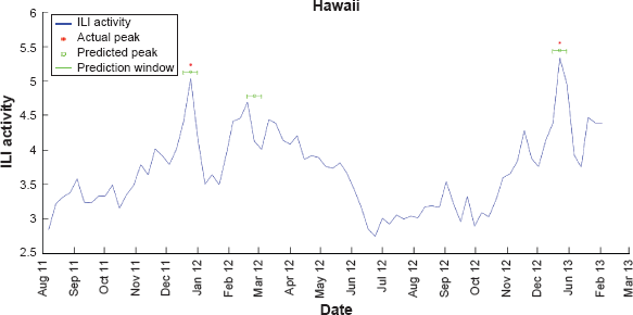
Weekly ILI activity versus time for August 2011 through March 2013 for military data in the state of Hawaii. The first and the third peaks were accurately predicted, but the second peak is a FP.

Figure 6

Weekly ILI activity versus time for August 2011 through March 2013 for military data in the state of Wisconsin. The two prediction windows correspond with the actual peaks.

Figure 7

Weekly ILI activity versus time for August 2011 through March 2013 for military data in the state of Mississippi. The second actual peak is missed by the prediction method and is a FN.

All the approaches have a very high NPV (>93%). One-Classifier 1 and One-Classifier 2 have superior PPV and specificity compared with the fusion approach. Specificity is important for keeping the false alarm rate to a minimum in order for the methods to be operationally useful. The sensitivity obtained by all the methods is between 60.9% and 69.2%. The best F_0.5 score (emphasizing PPV) is obtained by One-Classifier 2, and the best F₃ score (emphasizing sensitivity) is achieved by One-Classifier 1.

The performance of the FARM-based method was compared with some well-known classifiers, a decision tree (DT), a random forest (RF), and a support vector machine (SVM). Because DT, RF (as an ensemble classifier), and SVM are among the top 10 data mining algorithms according to Wu et al,³³ we selected these three classifiers to compare to the FARM method developed in this work. Weka³⁴ implementations were used for all three classifiers. A two-dimensional grid search was performed to optimize the classifier parameters on the training data set using a 10-fold cross validation. During the grid search, the average accuracy of these 10-folds is optimized by selecting the set of classifier parameters that lead to the highest average accuracy. In order to deal with unbalanced classes (many more nonpeak than peak examples) when computing the optimization error, weights (0.08 and 0.92 for nonpeak and peak, respectively) were introduced. The remaining parameters of the respective classifier models were used as default values from the Weka toolbox where applicable. Each trained classification model with the best parameters determined by the grid search was then evaluated on the test data to determine the classification accuracy. For the DT classification model, the minimum number of parameters per leaf and the number of folds for reduced error pruning were optimized. For the RF model, the number of trees and the number of random features per tree were optimized. For the SVM model with radial basis function kernel, the nonseparable cost parameter and the radial basis function gamma parameter were optimized. These optimized parameters are determined by the two-dimensional grid search in the Weka toolbox. The results for the alternative models are shown in Table 2.

Table 2

Performance of alternative classification methods on test data set.

METHOD	PPV	NPV	SENSITIVITY	F _0.5	F ₃
Decision tree	0.397	0.940	0.450	0.926	0.407	0.444
Random forest	0.553	0.922	0.236	0.979	0.436	0.250
SVM	0.247	0.971	0.798	0.738	0.287	0.652

Note: The best value of each performance metric is underlined.

Of these three methods, the RF has the highest PPV and specificity. The SVM has the highest sensitivity and NPV; however, it has a low specificity (73.8%), meaning that its false alarm rate is very high (26.2%). Comparing Table 2 with Table 1, One-Classifier 2 has a higher PPV and specificity than any method from Table 2. One-Classifier 1 has the highest NPV, and the SVM has the highest sensitivity as well as the lowest specificity (ie, highest false alarm rate).

Figure 8 shows F_0.5 and F₃ scores for all the methods. Because F scores combine PPV and sensitivity, they are a more robust way of assessing classifiers than PPV or sensitivity alone. One-Classifier 2 achieves the highest F_0.5 (emphasizing PPV). One-Classifier 1 has the highest F₃, while the SVM has the second highest F₃ (emphasizing Sensitivity). Overall One-Classifier 2 is the method that achieves both high F_0.5 and F₃, as well as low false alarm rate.

Figure 8

Comparison of F scores for the six methods used.

Conclusion

The DoD maintains a global laboratory-based surveillance program³⁵ as well as a near-real-time syndromic surveillance system to detect outbreaks of influenza and other conditions at military health-care facilities.³⁶ An additional capability to forecast influenza activity, integrated into this routine surveillance programs, could help guide DoD risk communication and resource allocation.

The data mining methods described in this article were used to produce a model for weekly influenza peak location prediction for each of 48 states in USA. Unlike an outbreak prediction model in which one predicts high or low likelihood of an outbreak during a specified period of time, this is a model for predicting when there would be seasonal peaks in influenza visits as a proportion of total health-care visits. It was complicated by the fact that there has not been an easily automated, consistent, and objective definition of what constitutes a seasonal peak. However, this model was able to utilize the results of previous efforts involving multiple and disparate types of data.^16–18 In addition, the practice of separating the data used in model development from that used for testing results in a much less biased estimate of prediction accuracy. The data mining techniques in this article take into account the very complex interrelationships that may exist among the large numbers of variables, while avoiding the pitfalls of model overfitting when using autocorrelation techniques. Because the desired outcome was an operationally useful model, our approach takes into account the fact that input data are not always immediately available on the date of collection. In addition, our approach paid special attention to minimizing FPs and FNs, so that the resulting model might be more operationally useful.

The One-Classifier methods that were predicting peaks four to six weeks into the future gave very encouraging results. The sensitivity of the methods ranged from 60.9% to 69.2%. The NPV and specificity were >97.5%, and PPV ranged from 50.9% to 60.3%. It is difficult to compare our results with those of Shaman et al¹³ due to the very significant differences in the prediction methodology, the data sources used, the method of counting lead time, and the spatial scales of the predictions. For example, their results were for predicting weekly Google Flu Trend estimates, while our results were for weekly peak ILI activity in military data. Also, our definition of the number of weeks ahead in the prediction differed from Shaman et al¹³ because our method takes into account the actual data availability. Shaman et al¹³ reported that the probability of accuracy (equivalent to PPV) of a peak predicted four to six weeks in advance ranged from approximately 0.4 to 0.5 for their high confidence predictions. However, because of the differences noted earlier, it is not possible to draw definitive conclusions about which method is more effective from these metrics. We also compared our results with those of three other popular data mining classifiers (DT, RF, and SVM). Overall, our data mining methods had a better PPV, NPV, and specificity, but the SVM had a higher sensitivity.

Our method for creating the prediction models was previously used for dengue fever^16,17 and malaria,¹⁸ but it can be used to create new models for different diseases. The use of widely available data enhances the generalizability of our method. This article has described a method for the prediction of peaks in influenza activity several weeks in advance for different regions in USA. Such predictions may provide public health officials and health-care providers with advance warning to plan mitigation procedures (eg, persuading people at a given location to get their influenza vaccinations before the predicted peak). By deploying such mitigation procedures before the peak, it may be possible to reduce morbidity and mortality from the seasonal influenza outbreak.

Author Contributions

Developed some of the prediction models, analyzed the results, and wrote portions of the article: ALB. Developed some of the prediction models, prepared the climatological data, and wrote portions of the article: BB. Prepared the climatological data and developed the DT, RF, and SVM models: EG. Prepared the influenza and case data and developed the peak identification algorithms: LM. Applied atmospheric science expertise and medical expertise to the analysis of the data and wrote portions of the article: SMB. Obtained the healthcare data, consulted on several nuances of the data, and wrote portions of the article: J-PC. All authors read and approved the final article.

Footnotes

Acknowledgments

The authors would like to express their appreciation to the US Armed Forces Health Surveillance Center for providing the epidemiological data and for supporting this study, particularly Dr. Rohit A. Chitale and Dr. Angelia Cost, and Sheri H. Lewis of the Johns Hopkins University Applied Physics Laboratory for helpful suggestions for the article. The authors wish to thank Matt Biggerstaff of the US CDC for his valuable input in identifying influenza peak weeks in military ILI data. The views expressed are those of the authors and do not reflect the official policy or position of the DoD or the US Government.

References

Medina

R.A.

, Garcia-Sastre

Influenza A viruses: new research developments. Nat Rev Microbiol. 2011; 9: 590–603.

Palese

Influenza: old and new threats. Nat Med. 2004; 10(12): s82–s87.

Gerdil

The annual production cycle for influenza vaccine. Vaccine. 2003; 21: 1776–1779.

Harper

S.A.

, Fukuda

, Uyeki

T.M.

, Cox

N.J.

, Bridges

; Advisory Committee on Immunization Practices (ACIP), Centers for Disease Control, and Prevention (CDC). Prevention and control of influenza: recommendations of the Advisory Committee on Immunization Practices. MMWR Recomm Rep. 2004; 53: 1–40.

Rello

, Pop-Vicas

Clinical review: primary influenza viral pneumonia. Crit Care. 2009; 13: 235.

Thompson

M.G.

, Shay

D.K.

, Zhou

. Estimates of deaths associated with seasonal influenza—United States, 1976-2007. MMWR Recomm Rep. 2010; 59(33): 1057–1062.

Taubenberger

J.K.

, Morens

D.M.

Pandemic influenza—including a risk assessment of H5N1. Rev Sci Tech. 2009; 28(1): 187–202.

Babin

S.M.

, Hsieh

Y-H

, Rothman

R.E.

, Gaydos

C.A.

A meta-analysis of point-of-care laboratory tests in the diagnosis of novel 2009 swine-lineage pandemic influenza A (H1N1). Diagn Microbiol Infect Dis. 2011; 69: 410–418.

Aquino

T.L.

, Brice

G.T.

, Hayes

. Influenza outbreak in a vaccinated population—USS Ardent, February 2014. MMWR Recomm Rep. 2014; 63: 947–949.

10.

Padin

D.S.

, Faix

, Brodine

. Retrospective analysis of demographic and clinical factors associated with etiology of febrile respiratory illness among US military basic trainees. BMC Infect Dis. 2014; 14: 576. doi: 10.1186/s12879-014-0576–2.

11.

Riley

, Ben-Nun

, Armenta

. Multiple estimates of transmissibility for the 2009 influenza pandemic based on influenza-like-illness data from small US military populations. PLoS Comput Biol. 2013; 9: e1003064. doi: 10.1371/journal.pcbi.1003064.

12.

Nsoesie

E.O.

, Brownstein

J.S.

, Ramakrishnan

, Marathe

M.V.

A systematic review of studies on forecasting the dynamics of influenza outbreaks. Influenza Other Respi Viruses. 2013; 8(3): 309–316.

13.

Shaman

, Karspeck

, Yang

, Tamerius

, Lipsitch

Real-time influenza forecasts during the 2012–2013 season. Nat Commun. 2013; 4: 2837.

14.

Chretien

J-P

, George

, Shaman

, Chitale

R.A.

, McKenzie

F.E.

Influenza forecasting in human populations: a scoping review. PLoS One. 2014; 9(4): e94130.

15.

US Centers for Disease Control and Prevention. Overview of Influenza Surveillance in the United States. US Department of Health and Human Services; 2013. Available at: http://www.cdc.gov/flu/pdf/weekly/overview.pdf. Accessed October 15, 2015.

16.

Buczak

A.L.

, Koshute

P.T.

, Babin

S.M.

, Feighner

B.H.

, Lewis

S.H.

A data-driven epidemiological prediction method for dengue outbreaks using local and remote sensing data. BMC Med Inform Decis Mak. 2012; 12: 124.

17.

Buczak

A.L.

, Baugher

, Babin

S.M.

. Prediction of high incidence of dengue in the Philippines. PLoS Negl Trop Dis. 2014; 8(4): e2771.

18.

Buczak

A.L.

, Baugher

, Guven

. Fuzzy association rule mining and classification for the prediction of malaria in South Korea. BMC Med Inform Decis Mak. 2015; 15: 47.

19.

Cawley

G.C.

, Talbot

N.L.C.

On overfitting in model selection and subsequent selection bias in performance evaluation. J Mach Learn Res. 2010; 11: 2079–2107.

20.

Vassiliadis

, Simitsis

, Skiadopoulos

Conceptual modeling for ETL processes. In: Proceedings of the 5th ACM International Workshop on Data Warehousing and OLAP; ACM; 2002: 14–21.

21.

US Centers for Disease Control and Prevention. Weekly US Influenza Surveillance Report; 2015. Available at: http://www.cdc.gov/flu/weekly/index.htm. Accessed October 15, 2015.

22.

Tamerius

, Nelson

M.I.

, Zhou

S.Z.

, Viboud

, Miller

M.A.

, Alonso

Global influenza seasonality: reconciling patterns across temperate and tropical regions. Environ Health Perspect. 2011; 119: 439–445.

23.

US National Oceanic and Atmospheric Administration. National Climate Data Center. Available at: http://www.ncdc.noaa.gov/land-based-station-data/quality-controlled-local-climatological-data-qclcd. Accessed October 15, 2015.

24.

Yau

M.K.

, Rogers

R.R.

A Short Course in Cloud Physics. 3rd ed. Oxford: Butterworth-Heinemann; 1989: 304. EAN 9780750632157, ISBN 0-7506-3215–1.

25.

US National Aeronautics and Space Administration. Goddard Earth Sciences Data and Information Services Center. Available at: http://mirador.gsfc.nasa.gov/. Accessed October 15, 2015.

26.

US National Aeronautics and Space Administration and US Geological Survey. Land Processes Distributed Active Archive Center. Available at: https://lpdaac.usgs.gov. Accessed October 15, 2015.

27.

Zadeh

Fuzzy sets. Inform Control. 1965; 8(3): 338–353.

28.

Kuok

C.M.

, Fu

, Wong

M.H.

Mining fuzzy association rules in databases. SIGMOD Rec. 1998; 27(1): 41–46.

29.

Agrawal

, Imielinski

, Swami

Mining association rules between sets of items in large databases. In: Proceedings of the ACM SIGMOD International Conference on Management of Data; May 1993: 207–216, Washington, DC.

30.

Liu

, Hsu

, Ma

Integrating classification and association rule mining. In: Proceedings of 4th International Conference on Knowledge Discovery Data Mining (KDD). New York: AAAI Press; 1998: 80–86. ISBN 1-57735-070–7.

31.

Quinlan

J.R.

C4.5: Programs for Machine Learning. San Francisco: Morgan Kaufman; 1993. ISBN 1-55860-238–0.

32.

Powers DMW. Evaluation: from precision, recall, and f-measure to ROC, informedness, markedness, and correlation. J Mach Learn Tech. 2011; 2(1): 37–83.

33.

, Kumar

, Quinlan

J.R.

. Top 10 algorithms in data mining. Knowl Inform Syst. 2008; 14(1): 1–37.

34.

Witten

I.H.

, Frank

Data Mining: Practical Machine Learning Tools and Techniques. 3rd ed. San Francisco: Morgan Kaufmann; 2011.

35.

Jeremy Sueker

, Blazes

D.L.

, Johns

M.C.

. Influenza and respiratory disease surveillance: the US military's global laboratory-based network. Influenza Other Respir Viruses. 2010; 4: 155–161. doi: 10.1111/j.1750-2659.2010.00129.x.

36.

Pavlin

J.A.

, Burkom

H.S.

, Elbert

. Combining surveillance systems: effective merging of U.S. Veteran and military health data. PLoS One. 2013; 8: e84077. doi: 10.1371/journal.pone.0084077.

Prediction of Peaks of Seasonal Influenza in Military Health-Care Data

Abstract

Keywords

Introduction

Materials and Methods

Predictor variables and their preprocessing

Military influenza case data

US CDC's influenza data

Environmental data

Methodology

Peak identification

Final peak algorithm

Steps in the prediction method

Metrics used for model evaluation

Results

Conclusion

Author Contributions

Footnotes

Acknowledgments

References