
Abstract
Motivation
A recurrent criticism is that certain bioinformatics tools do not account for crucial biology and therefore fail answering the targeted biological question. We posit that the single most important reason for such shortcomings is an inaccurate formulation of the computational problem.
Results
Our paper describes how to define a bioinformatics problem so that it captures both the underlying biology and the computational constraints for a particular problem. The proposed model delineates comprehensively the biological problem and conducts an item-by-item bioinformatics transformation resulting in a germane computational problem. This methodology not only facilitates interdisciplinary information flow but also accommodates emerging knowledge and technologies.
Introduction
A number of recent papers have identified ‘open’ problems in bioinformatics. From a computer science perspective, these problems have been classified broadly into those (i) related to the ‘central dogma’ (i.e. DNA to RNA to protein), (ii) related to data in general and (iii) simulating biological processes (Backofen and Gilbert, 2001). From a life science perspective, open bioinformatics questions are concrete questions, such as, ‘which structural RNAs are encoded in a genome?’ (Eisenberg et al. 2006; Goodman, 2002; Yu et al. 2004). Yet, there is a fundamental difference between the bioinformatics problems described above and the aim of this paper, which proposes a systematic procedure for constructing definitions of such problems.
For the most part, ‘how-to’ practices in bioinformatics address the application of software engineering and database management principles to computational issues. For example, Parker et al. (2003) proposed comprehensive management of information flow for large-scale genome projects through system-wide management of metadata and data dependencies across both biological and computational processes. This led to implementation of numerous integrated systems, commonly referred to as pipelines or workflows (e.g. Garcia Castro et al. 2005). Indeed, these efforts made significant contribution to bioinformatics ‘in-the-large’. Still lacking, however, are how-to-practices for bioinformatics problems ‘in-the-small’.
We propose a methodology for formulating bioinformatics problems by defining the cognate life and computational problems in an explicit and integrated fashion. The goal of this methodology is to guide development of bioinformatics tools that account for critical biology. Our work is much different from what is typically published in the field of bioinformatics. We focus on methods for formulating a problem rather then for solving an already formulated problem.
Methodology
Our procedure has three components: a biological model, a bioinformatics transformation and a computational model (Table 1). The biological model specifies a question of interest and defines the biological problem in a way that captures the breadth of the phenomenon. The bioinformatics transformation translates biological features and criteria into a set of computational rules, which, as a whole, circumscribe the biological problem. Finally, the computational model reformulates the problem mathematically by incorporating rules derived in the transformation and describes a computational approach to the initial biological question.
Methodology for formulating a bioinformatics model.

As an example of our methodology, we pose the biological question ‘which tRNAs are encoded in a genome?’ Information on tRNAs is available in the supplemental materials and in the literature (e.g. Marck and Grosjean, 2002; Paule and White, 2000; Sprinzl et al. 1998).
Biological Model
A biological model consists of a concise ‘biological question’ and a comprehensive description of the ‘biological knowledge.’ Both portions are critical to the entire bioinformatics model. The biological question is usually straightforward; for instance, the case example used here seeks to detect tRNA genes (i.e. a known phenomenon) in genomic sequences. In contrast, formulating the knowledge portion is more difficult requiring a comprehensive, taxonomically broad review of the life science literature and other available resources. As we detail below, the knowledge portion has three elements: (i) an abstract, ‘global’ definition of the phenomenon together with a textual exposé of observed scenarios, (ii) a comprehensive dataset of observed instances, and (iii) a description of yet unobserved, conceivable scenarios. Obviously, the state of knowledge about a particular biological problem determines how the question is formulated and how the biological phenomenon is described (see for example the early work on tRNA sequence and structure (Holley et al. 1965; Levitt, 1969)).
A sample biological model for tRNA gene identification is available in the supplemental Table S1. For the sake of simplicity, the model does not include more advanced criteria such as minimum free energy.
Definition and Observed Variation of a Biologicalc Phenomenon
One first provides a brief, abstract ‘textbook’ definition that views the phenomenon in a larger biological context, together with a typical scenario. Then, one should describe the extent and frequency of biological diversity, both within an organism and across taxa indicating both significant and minor differences. For tRNA gene identification, this may read as follows:
Transfer RNA molecules have two significantly different types of secondary structures, the cloverleaf and the two-arm. The more common structure consists of four stems (or three-arm) in the form of a cloverleaf ( Fig. S1 ). Yet, an unusual three-stem (or two-arm) type is common in certain animal lineages (Okimoto and Wolstenholme, 1990, Fig. S2). Notably, both types of tRNAs fold into a similar L-shaped tertiary structure ( Fig. S3 ). … A minor difference observed is the size of the D-arm loop (D-loop), which typically is 8 nt long but can be up to 10 nt long.
The description of the phenomenon should be comprehensive yet constrained to relevant features. For example, if the question involves identification of tRNA genes in genomic sequences, introns are relevant, but not so if the question solely addresses tRNA secondary structure. Similarly, mapping of a codon to an amino acid (the genetic code) is irrelevant for defining tRNA secondary structures, but relevant for identifying tRNA function.
Compilation of a Comprehensive Dataset
Concrete instances of a phenomenon make a description explicit and tangible. A compilation should span the breadth of taxonomic diversity and should contain a sampling of frequent occurrences as well as all known instances of rare and unique ones. As we discuss later, such a collection will be crucial for benchmarking bioinformatics tools.
Description of Conceivable Scenarios
Life scientists continually uncover novel occurrences of a given biological phenomenon, and not infrequently, these novelties fall within the expected range of diversity. To accommodate future discoveries within the framework of the biological model, one may include knowledge about biological structures and mechanisms that enable extrapolation of unobserved scenarios. Knowledge may be inferred from the same system, or from other systems or even other disciplines. For example, we know that a discontiguous molecule can assume the same structure or function as one that is contiguous. Thus, we can extrapolate that a tRNA gene could be encoded by multiple pieces, which are transcribed independently and join post-transcriptionally to form a functional structure. In fact, RNA ‘in pieces’ have been documented for ribosomal RNA (rRNA) of mitochondria from several eukaryotic groups and bacteria (Evguenieva-Hackenberg, 2005 and references therein) and rare examples for discontiguous tRNA genes have been reported as well (Randau et al. 2005; Soma et al. 2007).
A comprehensive biological model, as illustrated above, leads directly into the biological criteria of the next component, the bioinformatics transformation phase.
Bioinformatics Transformation
This component converts a biological description into a set of mathematical formulas. The translation process involves conversion of the biological knowledge description into biological criteria and transformation of these criteria into computational rules. A sample bioinformatics transformation for tRNA gene searches is available in the supplemental Table S2; note that all sample criteria below are excerpts from this table.
Biological Criteria
This first step converts the biological description into simple, concise verbal statements, termed biological criteria (BCs). A separate criterion is formulated for each characteristic of a feature, such as the length variation allowed for the stem of the D-arm (D-stem) of a tRNA, e.g.
The D-stem length is 3 or 4 nt.
In addition to this list of criteria, it is useful to group related statements (e.g. particular features or major variants) in order to add meaning and to aid organization. See Table S2 (section BC) for criteria for searching tRNA genes in genomic sequences.
After conversion to BCs, check statements for ambiguity. For instance, the criterion above indicates that the D-stem in tRNAs can vary in length. Yet, this statement is ambiguous since it is uncertain what kind of pairings make up a stem—only Watson-Crick pairings or also interactions such as G-U and G-G. To clarify this ambiguity, a new criterion that defines permissible pairings must be added:
Allowable nucleotide pairs: A-U, C-G and G-U.
More generally, clarification of the intended biological meaning may involve adding new or enhancing already formulated criteria.
Computational Rules
This step is the most crucial one of the bioinformatics transformation. Here, the BCs described above are converted into mathematical formulas, called computational rules (CRs). Generally, a single BC leads directly to a single CR, such as the one-to-one mappings exemplified by nucleotide pairings:
Valid nucleotide pairs (DNA) = {A-T, T-A, C-G, G-C, G-T, T-G}
and D-stem length variation:
3 <= | D-stem | <= 4
However, occasionally it may be necessary to combine several BCs to form a single CR (a many-to-one mapping). For example, a CR describing the length of a D-arm combines the following five BCs:
The D-arm forms a hairpin closed by a stem (pos. 10 to 25).
The D-stem length is 3 or 4 nt.
The D-stem pairing positions: 10-25, 11-24, 12-23 and 13-22. Note: if 13-22 do not pair, the numbering remains as though they are in the stem.
The D-loop length is 8 to 10 nt. If positions 13 and 22 do not pair, it increases to 7 to 11 nt.
The D-loop positions: 14, 15, 16, 17, 17a, 18, 19, 20, 20a, 20b, 21. Optional positions: 17a, 20a and 20b.
into a single CR:

Alternatively, a single BC may be utilized by several CR (a one-to-many mapping), such as permissibility of stem bulges used by each of the four stems (see Table S2; BC 3.1 is used by CRs 1.5, 1.6 and 1.9).
An important feature of the conversion step is the explicit mapping of BC to CR, which acts as a conduit that shuttles knowledge through the model. As laid out in the discussion, this mapping facilitates two important tasks: updating a bioinformatics model to accommodate new biological discoveries and assessing the biological capabilities of tools.
Some of the CRs represent the core of the problem, whereas others represent peripheral details. It is important to identify and mark as ‘key’ those features that are essential for the bioinformatics model. For the tRNA example, the basic cloverleaf and two-arm structures are critical features of the biological phenomenon. The search for intron-less tRNA genes may be central to a particular biological question. Finally, the T-arm and D-arm consensus sequences are essential for effective computational analysis. Rules marked as crucial receive special attention, not only during construction of the computational model but also later, during software development when infeasibility causes modification of the problem and removal of required rules (requirements).
Computational Model
The third phase of defining bioinformatics problems consists of reformulating the biological problem into a pure computational one. Unlike the two previous components, this phase does not devise a specific procedure, as techniques for defining a computational problem (model) are well established. Instead, we focus on what to include in such a definition.
First, a global problem definition should re-state the biological question as a computational problem. For example,
Problem: Given a DNA sequence, S, locate all genes, G, capable of forming a functional tRNA structure.
Second, we define a set of smaller problems (problem-set) that together describe a general approach satisfying the global problem. Each (smaller) problem should define a specific task and should state explicitly the CRs that apply to this particular problem. In addition, even the most trivial assumptions required by a problem should be stated explicitly in the definition. For example, assuming a four-nucleotide alphabet (for RNA sequences) lends itself to a highly efficient, bit-based computational approach. If the alphabet size would increase, this approach would be less effective and the problem itself may require revision. Third, each CR must be stated as a requirement for at least one (smaller) problem within a set. More challenging is determining all problems that rely on a given CR.
Obviously, more than one computational approach can address the same global problem; hence, alternative problem-sets can be formulated. For example, identifying tRNA genes using a machine learning approach may subdivide the problem in a manner that differs greatly from a purely deterministic, algorithmic approach. We recommend specification of all these alternatives as they facilitate development and comparison of software that use alternative computational techniques, be it hidden Markov models (Rabiner, 1989), Bayesian networks (Pearl, 1988), or rule-based systems (e.g. (Snyder and Stormo, 1993)).
Discussion
A bioinformatics model that is constructed according to the proposed methodology captures a problem in its entirety. This is achieved by specifying three separate yet inter-connected modules: a comprehensive biological description of the problem, a computational definition of the problem and an explicit transformation from one to the other.
Models constructed with our procedure provide a solid foundation for development, testing and comparison of analytical bioinformatics tools. Software development can focus fully on efficiency because the model ensures correct translation of the biology into a computational problem. Tools can be tested more easily, since comprehensive positive test data are readily available in the biological model. Once tools are available based on the same model, they can be compared to determine adherence to the model, performance against a benchmark dataset as well as time and space efficiency; all of these facilitate selection of the ‘best’ tool for a given analytical task.
Information Management and Software Engineering
Systematic procedures and information management principles are not new in bioinformatics. Informatics-leaning bioinformaticians have been applying these strategies for many years through explicit management of rules (‘requirements’), tracking of relationships between rules as well as data (‘dependencies’) and clear definitions of the extent of the problem (‘scope’). Currently though, such principles are applied predominantly to the informatics realm of bioinformatics rather than to bioinformatics as a whole, spanning both the informatics and biology realms.
Interdisciplinary Communication
For any interdisciplinary science, effective communication is a challenge. Bioinformatics has to deal with differences inherent to the life and computational sciences in terms of basic notions, ways of reasoning and scientific language. These differences present a substantial barrier to both comprehending and explaining ideas. Less obvious is a fundamental difference in conveying information. For instance, life science aims at extracting common patterns from the full breadth of natural diversity. In contrast, computer science aims at bounding a problem by defining assumptions, rules and constraints. Consequently, each side reduces the breadth of the problem through either generalizations or bounds. These reductions must be communicated.
The advantage of our methodology is that it facilitates interdisciplinary communication. First, the scientific language of a particular discipline is used to ensure accurate biological and computational models while translation from one model into the other occurs in a separate step. This provides explicit connections between the two models, connections that link specific biological criteria with specific computational constraints. As a consequence, tracing back a criterion/constraint from one model to the other becomes an easy task.
Changes in Knowledge and Technology
Biological sciences are about discovering new features of Life. Therefore, bioinformatics tools and resources need to incorporate new knowledge continually. For example, an early definition of gene regards it as a contiguous region on a chromosome that specifies an RNA or protein product. The subsequent discovery of alternative splicing and trans-splicing impacted fundamentally the assumptions underlying gene-finding tools.
Our methodology anticipates both incorporation of new knowledge and application of new technology. Advances in the life sciences can be accommodated because the model records relevant biological facts in a systematic fashion and specifies how they are interconnected with computational rules. Similarly, new computational technology can be accommodated because the model defines the scope and requirements for tool development. At most, a new problem-set needs to be added to the computational model. Construction of this new problem-set is simplified substantially by the computational rules contained in the transformation module.
Putting this Proposal into Practice
To allow cooperative model formulation and tool development, models should be openly available (pref. web-accessible). To accommodate new science, they should be easily expandable (e.g. managed in a database). Finally, new models need to reuse components of existing models (e.g. the description and the translated rules for nucleotide pairing). This not only reduces scientific effort and improves speed of model construction but also retains a consistent scientific representation across different bioinformatics models.
Conclusion
Bioinformatics needs standards and methodologies that span its entire breadth from biology to informatics. Establishment of systematic procedures is necessary to transform the ‘art’ of defining bioinformatics problems into a science.
Authors’ Contributions
AH conceived and refined the methodology. GB critiqued the methodology and made significant contributions both to the biological model and to comprehension of the methodology by life scientists. Both authors drafted the manuscript.
Footnotes
Acknowledgements
AH is a Canadian Institute for Health Research (CIHR) Strategic Training Fellow in Bioinformatics (Genetics Institute grant STG-63292). The Canadian Institute for Advanced Research (CIAR) is acknowledged for travel and interaction support for GB.
Supplemental Materials
Excerpts from a Bioinformatics Model for Trna Gene Identification
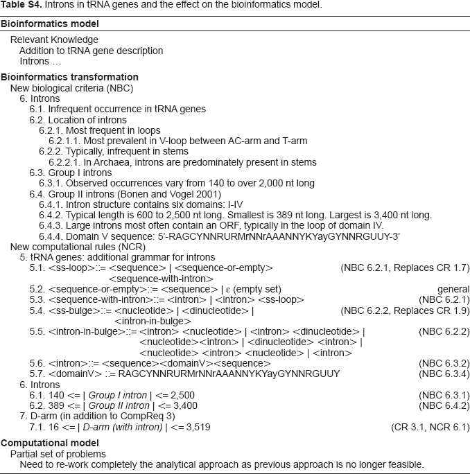
Introns in tRNA genes and the effect on the bioinformatics model.
| Bioinformatics model | |
|---|---|
| Relevant Knowledge | |
| Addition to tRNA gene description | |
| Introns … | |
|
|
|
| New biological criteria (NBC) | |
| 6. Introns | |
| 6.1. Infrequent occurrence in tRNA genes | |
| 6.2. Location of introns | |
| 6.2.1. Most frequent in loops | |
| 6.2.1.1. Most prevalent in V-loop between AC-arm and T-arm | |
| 6.2.2. Typically, infrequent in stems | |
| 6.2.2.1. In Archaea, introns are predominately present in stems | |
| 6.3. Group I introns | |
| 6.3.1. Observed occurrences vary from 140 to over 2,000 nt long | |
| 6.4. Group II introns (Bonen and Vogel 2001) | |
| 6.4.1. Intron structure contains six domains: I-IV | |
| 6.4.2. Typical length is 600 to 2,500 nt long. Smallest is 389 nt long. Largest is 3,400 nt long. | |
| 6.4.3. Large introns most often contain an ORF, typically in the loop of domain IV. | |
| 6.4.4. Domain V sequence: 5‘-RAGCYNNRURMrNNrAAANNYKYayGYNNRGUUY-3’ New computational rules (NCR) | |
| 5. tRNA genes: additional grammar for introns | |
| 5.1. <ss-loop>::= <sequence> | <sequence-or-empty> <sequence-with-intron> | (NBC 6.2.1, Replaces CR 1.7) |
| 5.2. <sequence-or-empty>::= <sequence> | ∊ (empty set) | general |
| 5.3. <sequence-with-intron>::= <intron> | <intron> <ss-loop> | (NBC 6.2.1) |
| 5.4. <ss-bulge>::= <nucleotide> | <dinucleotide> | <intron-in-bulge> | (NBC 6.2.2, Replaces CR 1.9) |
| 5.5. <intron-in-bulge>::= <intron> <nucleotide> | <intron> <dinucleotide> | <nucleotidexintron> | <dinucleotide> <intron> | <nucleotide> <intron> <nucleotide> | <intron> | (NBC 6.2.2) |
| 5.6. <intron>::= <sequencexdomainVxsequence> | (NBC 6.3.2) |
| 5.7. <domainV>::= RAGCYNNRURMrNNrAAANNYKYayGYNNRGUUY | (NBC 6.3.4) |
| 6. Introns | |
| 6.1. 140 <= | Group I intron | <= 2,50 | (NBC 6.3.1) |
| 6.2. 389 <= | Group II intron | <= 3,400 | (NBC 6.4.2) |
| 7. D-arm (in addition to CompReq 3) | |
| 7.1. 16 <= | D-arm (with intron) | <= 3,519 | (CR 3.1, NCR 6.1) |
|
|
|
| Partial set of problems | |
| Need to re-work completely the analytical approach as previous approach is no longer feasible. | |