Sage Journals: Discover world-class research

Abstract

In this review, we summarize the progress on coarse-grained elastic network models (CG-ENMs) in the past decade. Theories were formulated to allow study of conformational dynamics in time/space frames of biological interest. Several highlighted models and their underlined hypotheses are introduced in physical depth. Important ENM offshoots, motivated to reproduce experimental data as well as to address the slow-mode-encoded configurational transitions, are also introduced. With the theoretical developments, computational cost is significantly reduced due to simplified potentials and coarse-grained schemes. Accumulating wealth of data suggest that ENMs agree equally well with experiment in describing equilibrium dynamics despite their distinct potentials and levels of coarse-graining. They however do differ in the slowest motional components that are essential to address large conformational changes of functional significance. The difference stems from the dissimilar curvatures of the harmonic energy wells described for each model. We also provide our views on the predictability of ‘open to close’ (open→close) transitions of biomolecules on the basis of conformational selection theory. Lastly, we address the limitations of the ENM formalism which are partially alleviated by the complementary CG-MD approach, to be introduced in the second paper of this two-part series.

Keywords

normal mode analysis potential surface low-frequency motions GNM NMR X-ray B-factors

Introduction

Protein has a dynamic nature. Dynamics encoded in the evolutionally optimized (Leo-Macias et al. 2005) structures are coupled with catalytic chemistry in facilitating protein functions (Eisenmesser et al. 2002; Wolf-watz et al. 2004; Yang et al. 2005a). The ‘jiggling and wiggling’ atoms were understood in further depth when Koshland turned the ‘lock-and-key’ paradigm (Fischer, 1894) into an ‘induced-fit’ fever (Koshland, 1958) along with the first determined protein structure of sperm whale myoglobin by X-ray crystallography (Kendrew et al. 1958), in the same year. However, theoretical physics in long-wait could not characterize such an intrinsic property of proteins, microscopically, despite accumulated X-ray-solved structures in the 60's and early 70's, until computational facilities were mature enough to accomplish the first Molecular Dynamics (MD) simulation by Karplus and coworkers (McCammon et al. 1977). This seminal work described atomic motions following Newton's 2nd law with an empirical potential energy function and suggested a fluid-like nature in the interior of the protein (McCammon et al. 1977).

Not before long, in early 80's, Noguti T and Gō first examined the fluctuations of globular protein by a set of collective variables (Noguti T and Gō N, 1982). The new application of Normal Mode Analysis (NMA; Goldstein, 1950) to the protein BPTI deciphered the mode compositions of protein fluctuations (motions in the range <30 cm–¹ dominate the fluctuations) and described crystallographic temperature (B-) factors (the degree of uncertainty in atomic positions) surprisingly well (Gō et al. 1983; Brooks and Karplus, 1983). Domain motions at the active sites of lysozyme and ribonuclease were seen to occur in low frequency normal modes (Levitt et al. 1985). Within the small fluctuations at the equilibrium (reached after energy-minimizing the crystal structure according to a given potential energy function), NMA approximates the complicated potential (comprised of multiple contributions including bond stretching, angle bending, dihedral, electrostatics and van der Waals) surface harmonically. The second derivatives of the potential (with respect to atom displacements), the Hessian, is singular-value decomposed to obtain the normal mode shapes (eigenvectors) and frequencies (the square root of the eigenvalues). The analytical approach, solving the eigen-problem of the 3N_a by 3N_a Hessian matrix (N_a is the number of atoms in the protein) greatly reduces the computation time for obtaining the equilibrium dynamics of protein, as compared to MD. The low-frequency (slow) modes containing a certain degree of anharmonicity (Gō et al. 1983) not only are able to describe functional, configurational changes (Brooks and Karplus, 1985) but also help in the refinement of X-ray structures (Kidera and Gō 1992a, b).

NMA usually yields robust results, especially in the low frequency regime, because the results are not subject to statistical errors or sampling inaccuracies (unlike those retrieved from MD). However, MD, which makes no assumption about the underlying potential surfaces and allows transitions across energy barriers (which anharmonic motions include), is dearly needed to describe non-equilibrium dynamics involved in biologically important large conformational transitions, given a sufficient duration of simulations (Kitao et al. 1998; Arkhipov 2006a, b). However, the heavy computation of MD has limited its applicability to large biomolecular systems. The renaissance and further developments of coarse-grained MD (CG-MD) models, able to overcome the computational limit at a decreased resolution while maintaining key dynamic features of described systems (Tozzini, 2005), made possible simulations up to tens of microseconds (see our review on CG-MD in this series).

NMA gained unprecedented popularity in the late 90's along with two simplified schemes that resulted in a huge reduction of computational cost. One is the introduction of the Elastic Network (EN) concept, using a much simplified potential, being introduced by Tirion (Tirion, 1996) who proposed modeling molecules with their atoms within an interaction range being connected by Hookean springs of a universal strength. However, the first use of the word ‘network’, interpreting protein as junctions and elastic connections, was pioneered by Bahar and coworkers (Bahar et al. 1997) who took the idea from polymer science (Flory, 1976), using only C_α atoms to represent the protein. The description of proteins in reduced presentations is the so-called Coarse-Grained (CG) approach. Slow modes derived from both schemes were found to agree well with slow modes obtained from the standard NMA that uses a much more detailed potential. The saving of computational cost is tremendous: GNM, Bahar's model, required the diagonalization of a dimension-reduced Hessian, Γ (see below), which took 8.2 sec for T4-lysozyme (164 residues) on a single workstation (Bahar et al. 1997), as compared to 3 days by NMA (see Table 1) and much longer for nanosecond MD simulation for proteins of the same size to capture similar structural deformations.

Table 1.

Main features of CG-ENM.

EN Models	Nodes represent	Parameters in eq 1^ζ	Matrix Dimension^£	t_H or t_Γ^*
GNM (Bahar et al. 1997)	C_αs	E₀ = 0, γ = c, w_G = 1, w_T = 0, n = N, R_c = 7-15Å	N × N	1
CNM (Kondrashov et al. 2007)	C_αs	γ = 1 for \|i – j\| = 1and 0.1 for \|i – j\| ≠ 1; E₀ = 0, w_G = 1, w_T = 0, n = N; R_c = 4 or 4.5Å (ab denotes atom a in i and atom b in j that are the closest atoms between i and j)	N × N	1
ANM (Atilgan et al. 2001)	C_αs	E₀ = 0, γ = c, w_G = 0, w_T = 1, n = N, R_c = 10-15Å	3N × 3N	27
HENM (Hinsen 1998, 1999)	C_αs	E₀ = 0, w_G = 0, w_T = 1, n = N	3N × 3N	27
βGM (see Supplemental)	C_αs, C_βs	γ = 1 for C_α-C_α and 0.5 for C_α-C_β and Cg-C_β; E = 0, w = 0, w = 1, n = 2N, R = 7Å	3N × 3N	27
BENM (see Supplemental)	C_αs	E₀ = 0, w_G = 0, w_T = 1, n = N; γ and R_c are obtained in minimizing KLD with atomistic Hessian	3N × 3N	27
DNM (Kondrashov et al. 2007)	C_αs	E₀ = 0, w_G = 0, w_T = 1, n = N, $γ (\| {\vec{r}}_{i j}^{0} \|) = 1 / t r (H_{d}),$ d = R_c = 2.3, 3.3,5,7,9,11Å; ab denotes atom a in i and atom b in j	3N × 3N	27
RTB/BNM (Durand et al. 1994/Li and Cui, 2002)	blocks^§	H from detailed potential	6n_B × 6n_B	216
Tirion's (Tirion, 1996)^†	atoms	E₀ = 0, γ = c, w_G = 0, w_T = 1, n = N_a, R = 5.9Å	3N_a × 3N_a	27000
DWNM (see Supplemental)	C_αs	w_G = 0, w_T = 1, n = N, γ does not depend on $\| {\vec{r}}_{i j}^{0} \|$ but is a function of conformer m^¶; R_C = 13Å	N/A	N/A
PNM (see Supplemental)	atoms	w_G = 0, w_T = 1, n = N_a, γ does not depend on $\| {\vec{r}}_{i j}^{0} \|$ but is a function of conformer m^¶; R_C = 4.5-9.5Å	N/A	N/A
QEDM (see Supplemental)	quantized nodes	E₀ = 0, γ = c, w_G = 0, w_T = 1, n = N_n, R_c = 13Å	3N_n × 3N_n	27 (if N_n = N)
$E = E_{0} + \sum_{i, j = 1}^{n} \frac{γ (\| \vec{r_{i j}^{0}} \|)}{2} H (R_{c} - \| {\vec{r}}_{a b}^{0} \|) [w_{G} ({\vec{r}}_{i j} - {\vec{r}}_{i j}^{0}) • ({\vec{r}}_{i j} - {\vec{r}}_{i j}^{0}) + w_{T} {(\| {\vec{r}}_{i j} \| - \| {\vec{r}}_{i j}^{0} \|)}^{2}]$

†

Note that standard NMA has Hessian of the same size as Tirion's hence same diagonalization time.

with user-defined number of atoms.

when the structure is in the energy well of the conformer m at a given external parameter λ.

c is constant; ab = ij if not stated otherwise; i and j denote residues if n = N, or atoms if n = N_a; eq 1 is not applied for RTB.

the dimension of the square matrix H or Γ; N and N_a is the number of residues and atoms respectively; N ≈ 10 N_a; n_B = N if 1 residue per block; N_n is the number of quantized nodes.

t_H and t_Γ are the time taken to diagonalize the H or Γ (all the modes) using the standard subroutine; in relative unit as setting the time taken by GNM as unity.

Since then, the ease of programming and reduced computational cost due to the use of simplified potentials and smaller number of degrees of freedom resulted in wide-spread application of CG-EN models to deduce both the conformational dynamics of large structures and assemblies, including hammerhead ribozyme (Van Wynsberghe and Cui, 2005), CDK2/cyclin A (Dror and Bahar 2005), citrate synthase (Hinsen, 1999), hemoglobin (Xu et al. 2003), HIV reverse transcriptase (Bahar et al. 1999; Hinsen, 1999), hemagglutinin A (Doruker et al. 2002), aspartate transcarbamylase (Hinsen, 1999), F1-ATPase (Cui et al. 2004), an actin segment (Ming et al. 2003), GroEL-GroES (Keskin et al. 2002), the ribosome (Wang et al. 2004; Yang et al. 2006; Cui and Bahar, 2006) and viral capsids (Rader et al. 2005). Many intriguing biological systems as such, in a variety of sizes and extended applications (Tama et al. 2004; Leo-Macias et al. 2005) of ENMs have been carefully reviewed (Case, 1994; Kitao and Gō, 1999; Ma, 2005; Rader and Bahar, 2005; Tozzini, 2005). However, in-depth comparisons of the theories that underline the ENMs and their offshoots have been lacking.

In this review, ENMs (highlighted on Tirion's model, GNM, ANM and RTB/BNM) are illustrated in sufficient theoretical details: the basic hypotheses, the physical grounds, mathematical treatments and consequently achieved computational efficiency. The well comprehended ENM foundations serve to interpret data obtained from comparisons between predictions and experimental results, namely the observed equilibrium and non-equilibrium dynamics and those within ENMs themselves. Slow normal modes derived from different potentials and molecular resolutions are found robust within a subspace spanned by 5–6 dimensions (Nicolay and Sanejouand, 2006) but not on a one-to-one basis between the models.

NMA-based models show different levels of accuracy (Tama and Sanejouand, 2002) when examining the agreement between experimentally characterized large conformational changes and single slow-mode-driven structural deformations. These results together can be understood by motions taking place in harmonic energy wells with different curvatures approximated by different potentials and coarse-grained levels in the models. The profile of potential of mean force also helps in understanding the origin of a better predicted open → close transition than the closed → open counterpart by ENMs, using the concept of conformational selections (Ma et al. 1999; Dror and Bahar, 2006). Lastly, benefiting from the statistical study on comparisons of X-ray B-factors, RMSDs of NMR ensembles and GNM, we recently reported how experimentally characterized dynamics can comprise (and be affected by) motional components in different frequencies (Yang et al. 2007) and how the findings can be of use to understand the frequency dispersions of the models themselves. A separate review article on coarse-grained molecular dynamics simulations is presented back-to-back so as to address the non-equilibrium structural transitions that are beyond the reach of herein introduced EN models, given their basic hypotheses.

Theory—The ENM Models

Atomic-ENM

Tirion's model

To dispense with the problematic energy-minimization process prior to NMA while gaining computer efficiency, Tirion proposes a model to connect atom pairs with Hookean springs with a universal force constant γ (Tirion, 1996). The equilibrium structures are taken from the experimentally (X-ray or NMR) characterized structures assuming a zero energy. The resulting potential is a harmonic approximation that is much simplified than sophisticated potentials (Fig. 1a) used in NMA involving multiple bonded and nonbonded terms, which may or may not be harmonic depending on the instantaneous configurations of biomolecules in question. The total energy E of a molecule is

Figure 1

(a) The effect of simplified potentials. The energy landscape outlined by the conventional force field (detailed potential, as used by standard NMA) is drawn in thick lines. Simplified potential, (in thin lines) as used in Tirion's or CG-EN models, approximates the rugged potential surface crossing the local energy barriers. At coarse-grained level, the rugged potential can be described by RTB/BNM and the smoothed-out one by XNM {X = A, βG, C, D and HE …}. Despite the difference between the two potentials, equilibrium dynamics characterized by X-ray and NMR can be well described by both potentials from which the derived slowest modes cover the slowest ends of experimentally observed dynamics (see Discussion). In contrast, the slowest modes derived from the smoothed-out potential are slower than those derived from the detailed potential due to the narrower energy wells in the latter. As a result, large conformational transitions with high anharmonicity could be better predicted by the slowest modes derived from the simple elastic potential than by force-field-based potential. The blue long dashed line joins the equal energy points of two CG energy wells as described by PNM (see Supplementary Material). (b) Similarity of the shape of hierarchical global potential envelopes. The thick lines indicate the actual detailed potential. The blue dotted line approximates the local energy well as in the standard NMA or ENMs. Green dashed and red dot-dashed lines approximate the potential envelopes at a higher hierarchy. The fractal-like similarity between the curvature of the local well and those of the potential envelopes at a higher hierarchy could account for part of the reason why NMA-based models, assuming a minimal structural deformation and approximating the potential of mean force harmonically at the equilibrium, can often predict large conformational changes reasonably well.

E_{T i r i o n} = \sum_{i, j = 1}^{N_{a}} \frac{γ}{2} {(| {\vec{r}}_{i j} | - | {\vec{r}}_{i j}^{0} |)}^{2} H (R_{c} - | {\vec{r}}_{i j}^{0} |)

(1)

where ${\vec{r}}_{i j}^{0}$ is the vector connecting atoms i and j at equilibrium, defined in the PDB structures. Atoms i and j in the molecule that contains N_a atoms are connected by a Hookean spring if their separation is closer than a cutoff distance, R_c. H(x) is the Heaviside step function that is 1 when x ≥ 0 and zero otherwise. Force constant γ is chosen to optimally scale with NMA results or experimental measurements, such as the temperature (B-) factors of X-ray characterized structures (Tirion, 1996; Bahar et al. 1997). ENM reproduces the frequency spectrum and the eigenvectors of low-frequency modes of NMA at a 10^–3 computational cost of NMA's (Tirion, 1996). The improved efficiency is attributed to the absence of the initial energy-minimization step required before applying NMA and accelerated computations for the force constant matrix (second derivatives of the potential) due to the simplified energy function (Tirion, 1996). R_c was tested over values of 4.5, 4.9, 5.4 and 5.9 Å (including the sum of van der Waals radii, roughly 3.4 Å, for contacting atoms) and in all cases gave satisfactory results (Tirion, 1996).

CG-ENM

GNM

GNM, developed by Bahar and coworkers (Bahar et al. 1997), differs from Tirion's ENM in the following aspects. It was the first ENM that represents proteins with interacting ‘nodes’ at the amino-acid level (the CG scheme) while successfully reproducing X-ray B-factor data (Bahar et al. 1997), H/D exchange free energy costs (Bahar et al. 1998b) and ¹⁵N-NMR relaxation order parameters (Haliloglu and Bahar, 1999). Its potential employs the vector form of the displacement for node pair i and j under the isotropic assumption (<ΔX ΔX^T > = <ΔY ΔY^T > = <ΔZ ΔZ^T > = (1/3) <ΔR ΔR^T >, T is transpose, see the Supplementary Material):

\begin{array}{l} E_{G N M} = \sum_{i, j = 1}^{N} \frac{γ}{2} ({\vec{r}}_{i j} - {\vec{r}}_{i j}^{0}) \\ • (\vec{r} - {\vec{r}}_{i j}^{0}) H (R_{c} - | {\vec{r}}_{i j}^{0} |) \end{array}

(2)

or E_{G N M} (Δ R) = \frac{γ}{2} Δ R^{T} Γ Δ R (in matrix from)

(3)

where ΔR is the column vector of $Δ {\vec{r}}_{i};$ i runs over 1 to N for a protein of N residues; γ is again the uniform spring constant (force constant) and Γ is the N × N connectivity matrix (see Supplementary Material for details).

We can easily see the difference in the potentials of Tirion's and GNM. The inner product of vector differences, instead of the scalar difference of the i-j pair separations, penalizes not only the translational but also the rotational displacement, which partially accounts for its better B-factor agreement over other ENM models (Cui and Bahar, 2006).

The nodes in GNM are usually the C_α atoms of amino acid residues. R_c is generally set near or above 7 Å, the range of which covers the first coordination shell (Bahar et al. 1997; Cui and Bahar, 2006; see also Discussion). From the basics of Statistical Mechanics, one can easily derive the following results (see Supplementary Material for details)

\begin{array}{l} 〈 Δ {\vec{r}}_{j}^{2} 〉 = \frac{3 k_{B} T}{γ} (Γ^{- 1}) i i \\ 〈 Δ {\vec{r}}_{i} . Δ {\vec{r}}_{j} 〉 = \frac{3 k_{B} T}{γ} ((Γ^{- 1}) i j \end{array}

(4)

where $< Δ {\vec{r}}_{i}^{2} >$ is the ensemble average of the squared displacement of node i from equilibrium. Clearly, in GNM, only the magnitude square (the variance from the mean) of fluctuation is obtained due to the isotropic assumption and therefore the directions of the motions are not predicted. One should note that Γ has a rank of N-1. The diagonalization of matrix results in one zero eigenvalue and the associated trivial mode accounts for the rigid-body translation of the entire molecule. Therefore the Γ–¹ is a pseudo-inversion that is the sum of all the non trivial-modes. The covariance for pair i-j can be rewritten as

\begin{matrix} 〈 Δ \vec{r_{i}} \cdot Δ \vec{r_{j}} 〉 = \frac{3 k_{B} T}{γ} {(Γ^{- 1})}_{i j} \\ = \frac{3 k_{B} T}{γ} \sum_{k} {[λ_{k}^{- 1} u_{k} u_{k}^{T}]}_{i j} \end{matrix}

(5)

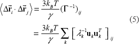
λ_k^–1 is the reciprocal of the k^th nonzero eigenvalue (the frequency square of the k^th mode) solved for Γ. The slowest mode (the 1st mode, with the lowest frequency) that has the most dominant contribution to the entire fluctuation is along the eigenvector u_k that is led by the biggest λ_k^–1. The slowest modes describe functional motions that are to great biological interests (Bahar et al. 1998a; Yang et al. 2005a). In addition, it is known from crystallography that the isotropic B-factors are proportional to the sizes of the fluctuations. That is

B_{i} = (8 π^{2} / 3) < {(Δ {\vec{r}}_{i})}^{2} >

(6)

Hence, B-factors can be predicted from GNM whereas the needed spring constant is obtained as scaling the predictions to match up with the experiment, namely the magnitude of B-factors, assuming internal atomic fluctuations fully account for structural uncertainties (Bahar et al. 1997; Cui and Bahar, 2006). The correlation between theories and experiments on the B-factors is found around 0.6 for a wide range of cutoffs and temperatures (Yang et al. 2006, supplementary material) and is 0.65 if crystal contacts are considered (Kundu et al. 2002).

CNM, an isotropic model extended from GNM, has reported a 0.74 correlation with B-factor profiles (Kondrashov et al. 2006) of 98 high resolution (< 1.0 Å) structures while employing a few modification schemes including crystal contacts (also reported previously by Kundu et al. 2002), residue contacts determined in atomic level while maintaining a N × N connectivity matrix (Γ) and enhanced force constant for backbone connections by a factor 10 (Kondrashov et al. 2006). More details can be seen in the Supplementary material.

ANM/Hinsen's CG-ENM

The ‘restoration’ of predicted fluctuations from 1-D (magnitude only) to 3-D came no later than 1998, pioneered by Hinsen (Hinsen, 1998). Hinsen's ENM (HENM) is carried out at the residual level, the potential adopts the same form as Tirion's except for the spring constant being in exponential decay with increasing residual pair separations. The decay corresponds to a weakened interaction between pairs far apart which simply reflects the physicochemical reality, although there is no specific reason why an exponential form has to be taken (Hinsen, 1998). The suggested form is

γ ({\vec{r}}_{i j}^{0}) = c \times \exp (- \frac{| {\vec{r}}_{i j}^{0} |^{2}}{r_{0}^{2}})

(7)

The parameter r₀ is set at 3-7 Å so as to best reproduce the low frequency normal modes obtained with the AMBER force field (Hinsen, 1998; Hinsen et al. 1999); c is a scaling factor. The design eliminates the need for assigning a cutoff distance (or interchangeably in this article, cutoff) as in other ENM models. However, an updated version of $γ({\vec{r}}_{i j}^{0})$ takes a stronger interaction for residue pairs in separation less than 4 Å, the range of which covers well the backbone neighbors. The spring constant for ${\vec{r}}_{i j}^{0}$ above 4 Å now decays with 1/r⁶. This format is proved to better approximate the long-time dynamics of proteins (Cui and Bahar, 2006).

Following a different path of derivation, Atilgan obtained the same result that differs from Hinsen's only at the spring constant being set as constant for simplicity hence the need to assign a cutoff distance of interactions (Atilgan et al. 2001). ANM is basically the CG version of Tirion's ENM except in assuming uniform mass for each amino acid (or bead) as done in HENM. HENM and ANM basically solve an eigen-problem involving a 3N × 3N force constant matrix (the second derivatives of the potential, see below), the Hessian (H) that contains N × N super elements H_ij (each super element is of dimension 3 × 3)

\begin{array}{r} H_{i j} (| {\vec{r}}_{i j}^{0} |) = \frac{- γ}{{| {\vec{r}}_{i j}^{0} |}^{2}} [\begin{matrix} x_{i j} x_{i j} & x_{i j} y_{i j} & x_{i j} z_{i j} \\ y_{i j} x_{i j} & y_{i j} y_{i j} & y_{i j} z_{i j} \\ z_{i j} x_{i j} & z_{i j} y_{i j} & z_{i j} z_{i j} \end{matrix}] \\ H (R_{c} - | {\vec{r}}_{i j}^{0} |) for i \neq j \end{array}

(8)

H_{i i} = - \sum_{j = 1}^{N} H_{i j | i \neq j}

(9)

The form is derived from the second derivatives (with respect to the node displacements) of the potential. Here, x_ij, y_ij and z_ij are the components of ${\vec{r}}_{i j}^{0}$ . Six zero eigenvalues and associated eigenvectors obtained from diagonalization of the Hessian stand for the six degrees of freedom of rigid-body translation/rotation. The 3N-6 non-trivial eigenvectors that give sizes and directions of motions for nodes in each mode are obtained.

As for the efficiency, Hinsen's Hessian is less sparse than ANM's and therefore takes minimal advantage of the regular sparse matrix solver hence a slower computation than ANM, despite similar low-frequency modes being obtained in both (Cui and Bahar, 2006). DNM, a modified version of ANM, which uses distance-dependent force constants (hence the name Distance-based Network Model; Kondrashov et al. 2007b), was reported to have an improved prediction on Anisotropic Displacement Parameters (ADPs) over ANM (Kondrashov et al. 2007). More details are available in the Supplementary Material.

RTB/BNM

The collective motions seen in low-frequency normal modes often occur at the levels of residues, secondary structures, or even domains. It provides the physical motivation to describe such motions as rigid-body translations/rotations of blocks (RTB) of atoms (Fig. 2a), the mathematical treatment of which is the projection of the 3N_a by 3N_a atomistic Hessian into a small 6n_B × 6n_B block-matrix, where N_a is the number of atoms and n_B is the number of blocks chosen for the molecule in question (see below).

Figure 2

(a) Each block in the molecule is a rigid body that is subject to local translations/rotations (T/R) described by 6 T/R eigenvectors. The figure is reproduced from Durand et al. (1994) (b) The atomic Hessian matrix is expressed in a reduced basis for each coupled or diagonal block. Block i and j has N_a,i and N_a,j atoms, respectively. U_i (part of the P matrix) is a N_a,i by 6 matrix that consists of 6 T/R vectors, representing the rigid body motions of block i. The atomic Hessian elements for blocks i and j is projected to a 6 × 6 reduced Hessian H_ij^b using the equation H^b_ij = U_i^TH_ijU_j. Superblock, used in BNM, comprises several blocks. The Hessian elements within each superblock is computed on the fly and then projected to reduced dimension with P. The figure is reproduced from Durand et al. (1994) and Li and Cui, (2002).

Although Bahar physically coarse-grained proteins, Sanejouand and co-workers were among the first to coarse-grain the protein at the mathematical level as early as 1994 by breaking up the protein into residue blocks (the building-block approach) while introducing rotation-translation basis into the atomic Hessian (Durand et al. 1994). With the eigen-problem solved at a reduced dimension, RTB makes the dynamic analyses of supramolecules computationally tractable, in the same spirit as other CG models. The analysis on a series of proteins of various sizes is made possible and demonstrates a good reproducibility of standard NMA results especially in the low-frequency spectrum. (Tama et al. 2000).

Atomistic Hessian herein, H, of size 3N_a × 3N_a, is first computed and stored. The projection matrix, P, of size 3N_a × 6n_B, comprising six local translation/rotation vectors of blocks (and the degrees of freedom of each block sum up to N_a, see Fig. 2b), is prepared for the subsequent projection (the detailed formula for P can be found in Li and Cui, 2002). A block, although can be a cluster of any number of atoms, is often chosen to consist of atoms of a single or several consecutive residues in sequence (Tama et al. 2000). The projected Hessian,

H_{b} = P^{T} H P

(10)

of size 6n_B × 6n_B, usually 25 fold smaller in memory storage and therefore 125 fold faster in computation than H (consider 1 block = 1 residue ≈ 10 atoms and in one dimension, 3N_a/6n_B ≈ 5), is diagonalized to give 6n_B eigenvalues and eigenvectors (Fig. 2b). The corresponding 3N_a atomic displacements can then be approximated by projecting the solutions from a reduced dimension back to the full dimension as

A_{p} = P A_{b}

(11)

Here, A_p is the approximated eigenvector matrix (3N_a × 6n_B) of H, which consists of 6n_B slowest normal modes and can be projected from A_b (6n_B × 6n_B), the eigenvector matrix of H_b, with multiplying the projection matrix P.

The Block Normal Mode (BNM) approach is basically the same as RTB, yet employs a better computational implementation such that the required atomic Hessian elements for constructing the ‘blocks’ are computed on the fly and the big H never has to be stored (Li and Cui, 2002).

Note that approaches such as RTB/BNM are different from other CG-EN models on two aspects. RTB and BNM inevitably need the preliminary energy minimization, as the standard NMA, before building the atomic Hessian elements. Moreover, the harmonic potential they describe, despite being blocked, is less smoothened out than models such as GNM or ANM that have a physically coarse-grained elastic potential (Fig. 1a, see also Discussion).

Other EN Models such as backbone-enhanced elastic network model (BENM), β Gaussian Model (βGM), quantized elastic deformation model (QEDM), plastic network model (PNM), double-well elastic network model (DWNM) and models based on linear response theory, also to readers’ great interest, are introduced in the supplementary material. Their potentials and resulting properties of Hessians are summarized in Table 1.

Online Access of the Cg-En Models and NMA Results

Web services for GNM (Yang et al. 2005b, 2006), ANM (Eyal et al. 2006), NMA (Wako et al. 2004) and others (see a review by Xiong and Karimi 2007) are developed in recent years to facilitate a high-throughput analysis on conformational dynamics via ‘biologist-friendly’ interfaces.

Discussion

The section is composed to first analyze the basic assumptions of EN models, the nature of the normal modes that are derived from them and the nature of the experimental observations that are often compared with ENM-derived predictions and eventually answer the question—which EN model is the ‘best’?

The Essence of the Cutoffs

The cutoff distance (R_c) is usually set to take account the physical reality and save the computation cost on those negligible interactions for atom pairs far apart (Leach, 2001). For Tirion's ENM or ANM, R_c was first chosen to best reproduce the frequency spectrums of NMA or GNM respectively (Tirion, 1996; Atilgan et al. 2001) whereas in GNM, it was chosen to include the contacts within the first coordination shell defined by the C_α-based radial distribution function (Bahar et al. 1997). However, Yang has shown that a range of R_c from 7 to 15 Å simply renders statistically identical correlations with B-factors over 1250 nonhomologous proteins (Yang et al. 2006). The robust isotropic nature of time-average fluctuations was also reported in Eyal and Kondrashov's studies (Eyal et al. 2007; Kondrashov et al. 2007).

Taking the correlation with B-factors of Protein/DNA/RNA biocomplexes as a function of residue-residue contact distance (R_c), nucleotide-nucleotide contact distance (R), residue-nucleotide contact distance ((R_c + R_p)/2) and the number of beads (from 1 to 3) used to represent a nucleotide given one bead per protein residue, Bahar and coworkers found that the result was maximized at R_c = R_p = 7 Å given 3 beads per nucleotide which is known to be roughly 3 times heavier than an amino acid (Yang et al. 2006). The setting of 3-nodes-per- nucleotide (P, C4* in the sugar and C2 in the base) plus 1-node-per-residue also made nodes distributed more evenly within the shape of the molecule than other settings.

The use of cutoff distance in these models simply serves to measure the local packing density (Halle, 2002) which is the counts within a fixed volume (consequently a fixed cutoff distance). The concept herein has been widely used in classical/statistical mechanics for sampling particle properties at a coarse-grained level (Nitzan, 2006). Mixed cutoff schemes, as first attempted in the study above, do not sample such a density in equal volume while the packing density is known to have a dominant contribution to residue fluctuations (Halle, 2002; Cui and Bahar, 2006; Yang et al. 2006). Biased local density sampled leads to an unphysical Hessian that preserves no cutoff information, causing impaired predictions. Hence, as long as the employed cutoff renders a good representation of local features (not too small for nodes to ‘see’ only the backbone neighbors or too wide for all the nodes to be connected together), similar prediction results for isotropic data are faithfully obtained. We should also note that anisotropic vibrations are more sensitive to employed cutoffs hence models based on detailed potentials giving better predictions for ADPs than ANM does (Kondrashov et al. 2007).

Slow Modes Rather than Fast Modes are Robust

Nicolay and Sanejouand asked how many normal modes are needed for a given NMA-based model to describe the normal modes obtained from other protein models that use different potential and coarse-grained schemes. The results suggested that 5–6 Tirion's EN modes in the lowest frequencies are enough for the description of a few slow modes obtained with the all-atom CHARMM potential (Nicolay and Sanejouand, 2006). The invariant nature of a robust subspace spanned by 5 to 6 normal modes was again seen in the crosscheck over the other two CG-EN models, including ANM (Nicolay and Sanejouand, 2006). Moreover, low-frequency subspace from essential dynamics analysis is found to be spanned well by a few low-frequency normal modes (Rueda et al. 2007). In fact, similar slowest (1st) modes can be obtained through a hierarchy of coarse-grained (HCA) schemes for a given EN model (Doruker et al. 2002; Ming et al. 2002).

Proteins with a similar architecture encode similar conformational dynamics, as natural as one might expect. However, slow components are more robust against structural variations than the fast ones (Keskin et al. 2000; Cox et al. 2007). Quantitatively speaking, a 2.1 Å RMSD between two structures of the same protein, separately solved by X-ray and NMR, gives a correlation of 0.94 (statistical average) between their slowest-mode profiles that are derived from GNM (Yang et al. 2007). The insensitivity to minor structural changes is understood to stem from the collective nature of the low-frequency modes. The collective oscillation is a joint effect of many interacting pairs, summed up to approach a universal form that is governed by the central limit theorem, regardless of the details of pair positions or potentials (Tirion, 1996; Atilgan et al. 2001). Another interesting observation made by ANM combined with a structural perturbation method is that low modes are robust to sequence variations or in other words, insensitive to mutations (Zheng et al. 2006).

Magnitude Rather than Directions of Fluctuations is a Robust Feature

On the other hand, the fluctuation magnitude is better predicted than the direction of the motions. Kondrashov used five different CG-EN models including BNM using the CHARMM potential to examine their agreement with crystallographically characterized isotropic and anisotropic dynamics (Kondrashov et al. 2007). The result showed almost the same correlation between the predicted time average magnitude and the reported isotropic fluctuations for the five models, whereas the predictions on the reported directions of motions are shown to be model-dependent (Kondrashov et al. 2007). Bahar and coworkers confirmed the same observation in a systematic study on a collection of ADPs (see the DNM model in Theory) reported in 93 high-resolution PDB structures and found the sums of the diagonal elements (the magnitude) in the inverse Hessian to agree better with experiment than the off-diagonal elements (indicating the directions) (Eyal et al. 2007). In fact, Kondrashov and Eyal found experimentally reported ADPs are highly refinement package dependent (average anisotropy given by Refmac is 0.64 and is 0.51 by SHELX; Kondrashov et al. 2007) and greatly sensitive to the forms of crystal packing symmetry (substantial difference in ADPs reported for the same proteins packed in different space groups; Eyal et al. 2007). One should note that a model that is tuned to best predict the directions of motions does not necessarily best describe the magnitude of the motions (Kondrashov et al. 2007; Eyal et al. 2007), indicating strong experimental artifacts. Use of ANM to predict RMSDs of the 64 NMR ensembles also found better agreements in the magnitude (0.69) rather than the directions (0.62) (Yang et al. 2007). The better reproducibility in the magnitude rather than the directions is not only seen between experiment and theory but also between theoretical results (Cox et al. 2007).

Understanding Dynamics Hidden in the Electronc Cloud

In X-ray crystallography, the iso- and anisotropic B-factors are obtained via a fitting process to position the atoms that best represent the electron density distribution. They have been understood more as the structural uncertainty (or errors) rather than quantization of dynamics. The difficulty to fully count B-factors as dynamic quantities is that they contain strong contributions from the crystal packing. In the early 90's, Kidera and Gō have shown through the use of the standard NMA that the external contribution (58%) to the B-factors are actually larger than the internal ones (42%) in human lysozyme (Kidera and Gō 1992 a, b). As EN models describe internal fluctuations, only, how can a model like GNM score a good correlation with B-factors?

The reason is explained as follows. We have to note that GNM is a 1-D model that motions are carried out in the 1-D magnitude space with a rigid-body translational shift (the trivial mode led by a zero eigenvalue) for the entire molecule. B-factors can therefore be fitted as

B_{i}^{i s o} = c_{t r a n s} + c_{N M} \sum_{k = 2}^{N} {[λ_{k}^{- 1} u_{k} u_{k}^{T}]}_{i i}

(12)

As a result, the correlation between the profiles (as a function of residue index) of $B_{i}^{i s o}$ and $\sum_{k = 2}^{N} [λ_{k}^{- 1} u_{k} u_{k}^{T}]$ will not be changed no matter how big or small the constant c_trans is. Parameter c_NM is a constant that contains γ. On the other hand, for 3-D models like ANM, contributions from rotational rigid body motions should be considered.

\begin{array}{r} B_{i}^{i s o} = c_{t r a n s} + c_{r o t a t e} \times ‖ {\vec{r}}_{i} - {\vec{r}}_{m c} ‖^{2} \\ + c_{N M} \sum_{k = 2}^{N} {[λ_{k}^{- 1} u_{k} u_{k}^{T}]}_{i i} \end{array}

(13)

Where ${\vec{r}}_{i}$ and ${\vec{r}}_{m c}$ are the position vectors of atom i and mass centroid of the molecule respectively. This is the minimal fitting scheme using the least parameters. Of course, due to the heterogeneity in the crystal, popular models (Winn MD et al. 2001) using more parameters is quite understandable. Also, if considering how each mode could be excited by different crystal packing forms, a modified version of the above equation would be to parameterize the contribution of each normal mode (Song and Jernigan, 2007). Both the rigid-body rotation $({‖ {\vec{r}}_{i} - {\vec{r}}_{m c} ‖}^{2})$ and internal vibrations $({\sum_{k = 2}^{N} [λ_{k}^{- 1} u_{k} u_{k}^{T}]}_{i i})$ contribute to the shape of the theoretical profiles. However, most of the comparisons between ENM-derived internal fluctuations and B-factors are done without considering such a contribution of rigid-body rotation (Kondrashov et al. 2007; Eyal et al. 2007). This could be part of the reason that 3-D ENM models compare slightly worse with B-factors than 1-D models do (such as GNM and CNM) on top of the acknowledged fact that GNM penalizes the rotational deformation when 3-D ENMs do not (see the GNM subsection in Theory; Bahar, 1997; Cui and Bahar, 2006).

Understanding NMR Characterized Dynamics

NMR characterizes protein structure and dynamics in the solvated state. Predictions from ENMs have been in a good agreement with such NMR-characterized dynamics, namely the order parameters (Yang and Kay, 1996), derived from NMR relaxation data (Haliloglu and Bahar, 1999; Ming and Bruschweiler, 2006). Accordingly, Chen recently uses such quantity as a benchmark to rationally select ensembles from MD snapshots that best reproduce the order parameters (Chen et al. 2007). In addition, it is interesting to see that GNM has a 0.74 correlation with the RMSDs of NMR ensembles as opposed to a 0.59 correlation with the B-factors of their X-ray counterparts (same proteins alternatively solved by X-ray). Deleting the slowest GNM mode that contributes to the time-average fluctuations and then comparing with the same aforementioned quantities leaves the correlation with X-ray unchanged but dramatically decreases the correlation with NMR, indicating the differences in the spectrum of modes accessible in solution and in the crystal environment. Specifically, large amplitude motions sampled in solution are subdued in the crystalline environment of X-ray crystallography due to the restraints from crystal contacts (Kundu et al. 2002) and low temperatures (Yang et al. 2007).

Refined NMR conformers are obtained from simulated annealing runs and energy minimization (Brünger, 1991a, b) over the detailed potential surface defined by the target function (Schwieters et al. 2003) that comprise both the empirical force field and NMR restraint-derived penalty terms (Yang et al. 2007). Although more studies are needed for a clear understanding of the correlation between NMR and GNM, surprisingly, anharmonic procedures as such to populate the NMR conformers in distributed local wells can be approximated by GNM that uses simplified elastic potential. The statistical result suggests NMR ensembles should not be deemed solely as the range of ‘errors’ in structure determination but more as a set of conformations accessible to the molecule in question under the experimental conditions.

Open-to-close Transitions Being Better Predicted than Contrariwise

There have been studies showing protein open→close transitions (meaning that the open form of the structure is used by NMA- or MD-based models to generate low frequency normal or PCA modes in order to compare with experimentally identified structural transition vectors) are better predicted than their close→open counterparts in quite a few systems including adenylate kinase (Temiz et al. 2003; Miyashita et al. 2003; Maragakis and Karplus, 2005), citrate synthase (Hinsen, 1999), LAO binding protein (Tama and Sanejouand, 2001), hemoglobin T→R2 transition (Xu et al. 2003) and E. coli ABC Leu/Ile/Val transport system (Trakhanov et al. 2005). A systematic study over 10 structure pairs (open/close) further confirmed this intriguing tendency (Tama and Sanejouand, 2001). The statistics in average, when ANM is used, is 0.58 and 0.43 for open→close and close→open, respectively (Tama and Sanejouand, 2001). The trend does not seem altered when different models or potentials are used. For adenylate kinase, which undergoes large, functional conformational transition that is crucial for life-related signaling cascades when triggered by hormone or metabolite cues, the correlations between prediction and experiment for open→close transition when simplified or detailed potentials are used in the ENM are 0.62 and 0.53 respectively, while those for close→open are 0.38 and 0.37, respectively (Tama and Sanejouand, 2001).

The reason is explained in Figure 3. The concept of conformational selection (Ma et al. 1999; Dror and Bahar, 2006) states that protein binds its ligands/substrates at its preexisting equilibrium state and therefore a certain conformational state is ‘selected’ or being ‘locked up’. Hence, an unbound structure has natural tendency to deform along the slowest normal modes to a state that resembles the bound conformation before the ligand comes in and locks the very state. For structure in the bound state, new contacts (or bonds) are formed not only at the binding site but also throughout the distal domains. The newly defined architecture due to altered pair contacts gives a Hessian distinct from that of the open state. The ‘open’ structure is therefore hardly found along the smoothest path (at the lowest energy cost) of the narrowed energy well (see Fig. 3) of the ‘close’ structure. The disallowed returning journey back to ‘open’ is permitted again upon the ligand release/bond breakage or the second incoming chemical cues.

Figure 3

Conformational selection (Ma et al. 1999; Dror and Bahar, 2006) explains why open → close is easier predicted than close → open. Assuming only the protein takes the conformational change but ligand does not in either the bound or unbound state, the binary system, ligand + protein, evolves along the energy landscapes defined by (1) protein conformational change (with or without the contact of ligand) and (2) the binding energy ΔG, only. The conformational change is approximated harmonically by either atomic- or CG-ENM. “Close bound” state herein is referred to as ‘close state’ in the literature. Protein at the ‘open’ state access a close but unbound state (Dror and Bahar, 2006) along the smoothest deformational path (thin line), namely the slowest few normal modes. The protein in the disfavored “close unbound” state may further change the conformation a bit as being ‘induced’ by the ligand which then draws the whole binary system down to a new energy funnel at the big ΔG relief, in the end of the ligand docking. Since the architecture of protein is redefined by the newly formed contacts (Fig. 1 in Tama and Sanejouand, 2001), in either the “close unbound” or “close bound” (more so) state, the energy profiles (dash and solid lines, respectively) change their shape and curvature (mostly narrower) and the groups of atoms that undergo collective motions in the path open → close may not be identifiable again in the path close → open as NMA being performed on both of these close states. Not until the catalytic reaction on the substrate is complete or the ligand is released upon other chemical cues and in turn ‘pushes’ the structure back open, anharmonically, does the protein architecture resume its ‘open’ state again.

Which CG model is the Best?

Since the late 90's people regained interest in NMA-based models, due to aforementioned simplifications, the initial of ‘X'NM has had a decent coverage over the 26 alphabets. A natural question that arises is: which one is the best? To answer this, we shall first define what ‘good’ is? For a long time, ‘good’ has been acknowledged as reproducing (1) results derived from detailed, atomistic potentials (NMA or MD) and/or (2) experimental results (spectroscopic data, free energy measurements etc). Depending on the type of questions in study, (1) and (2) are not necessarily always the same thing (see below).

Great efforts have been expended on CG-models to reproduce the results obtained from detailed (force-field-based) potentials (Hinsen, 1998; Tama et al. 2000; Li and Cui, 2002). The coarse-grained schemes therein seem motivated from a purely computational point of view. Is there any physical insight gained from coarse-graining and its concomitant simplified potential used, besides the mathematical convenience?

Simplified and Detailed Potentials

Although slow normal modes derived from different potentials and molecular resolutions are found robust within a subspace spanned by 5-6 dimensions (Nicolay and Sanejouand, 2006), the correspondence between modes of different models is not on a one-to-one basis. Kondrashov examined five CG models and found that BNM/RTB (using detailed potential) gave lower mode-to-mode correspondences with the other three CG-EN models investigated in the study than those within CG-ENM themselves: 15-25% lower in the lowest 17 modes (Kondrashov et al. 2007: Fig. 3, statistical results from 83 proteins). In fact, ANM and BNM showed the largest differences in the study: ‘only’ 0.6 to 0.7 agreements were seen between them in the slowest three modes (Kondrashov et al. 2007). Tama and Sanejouand also demonstrated that the simple potential used in ANM actually outperformed the detailed one used in RTB in predicting the protein open→close conformational transitions for 4 out of 5 proteins (Tama and Sanejouand, 2001).

On the other hand, ANM and BNM show identical accuracy in reproducing isotropic displacements (B-factors) although BNM outperforms ANM in predicting ADPs (Kondrashov et al. 2007). Note that to predict B-factors or ADPs requires a summation of all the normal modes. A question that follows is why the sum of all the modes of ANM and BNM agree with B-factors equally well when they differ in their slow modes that should contribute the most to overall fluctuations?

Recently, Bahar and coworkers demonstrated that deleting the slowest mode of GNM does not deteriorate its theoretical agreement with crystallographic B-factors due to the slowest motions being restrained by crystal contacts at low temperature (Yang et al. 2007). A subsequent study along this line, for the same set of 64 proteins, has shown that consecutive deletions of the slowest 8th modes in ANM and > 140th modes in Tirion's model are needed before a reduced agreement with B-factors can be seen (unpublished data). This indicates that the lowest frequency components are not required for a good prediction of isotropic motions of molecules in the crystal although adding those components back barely (if any) decrease the correlations. This more or less explains why almost all the models give reasonable predictions on B-factors.

Coarse-grained and fine-grained ENMs

GNM, ANM and Tirion's ENM have different curvatures in their ‘slowest’ harmonic wells, the curvatures of which are simply captured by the second derivatives of the potentials in the Hessian(s) spanned by the slowest mode(s). However, they show nearly identical accuracy to reproduce B-factors (Eyal et al. 2007). The reason of that can be understood similarly as for simplified and detailed potentials. The study in influenza virus hemagglutinin A (Doruker et al. 2002) nonetheless shows that reduced representations of molecules produce similar shape of slow mode profiles. In fact, the slower the modes are, the more similar they are with each other across a hierarchical, reduced representation. Other evidence shows that the slowest 50 modes derived from fine-grained model (Tirion's) or from coarse-grained model (ANM) can drive the docking of high-resolution structures into the corresponding low-resolution electron-density maps (Tama et al. 2004; Delarue et al. 2004; Hinsen et al. 2005) equally well in the Normal Mode Refinement (Kidera and Gō, 1992a, b).

Harmonic Approximations of Potentials Used in ENMs

The observed difference between detailed-potential- and simplified-potential-derived normal modes is a natural result of harmonic approximations taken at energy minima with different curvatures. The difference remains even when the atomistic Hessian being projected into reduced subspace in the RTB/BNM.

So, which model is the best? For structures staying near their equilibrium states where the dynamics can be characterized by NMR or X-ray, almost all the models perform equally well. GNM and Tirion's ENM predict the size of RMSDs of NMR ensembles equally well (0.74) and slightly outperform ANM (0.68) (Yang et al. 2007) whereas GNM, ANM, Tirion's ENM, βGM and standard NMA predict isotropic B-factors (or the trace magnitude of the anisotropic fluctuations) equally well with a correlation from 0.55 to 0.59 when the crystal contacts are not taken into account (Yang et al. 2006; Eyal et al. 2007).

Large conformational transitions that span across multiple local wells or a hierarchy of energy wells are beyond the reach of harmonic approximations discussed herein. Atomistic- or CG-MD are better approaches to study such transitions (usually accompanied with partial unfolding; see Okazaki et al. 2006) although CG-ENM could still give reasonable predictions along their slowest motional path due to the similarity of the shape of hierarchical global potential envelopes and the approximations by simplified potentials (Fig. 1b; Hinsen, 1998; Tama and Sanejouand, 2001; Tama et al. 2004; Cui and Bahar, 2006), which exhibits a fractal character. More rigorous systematic studies are needed to examine how the difference in the slowest normal modes from different CG-EN models impacts the prediction accuracy in dynamic events at an extended time scale.

Note that slow modes obtained from Principle Component Analysis (PCA) on MD trajectories can well agree with the slow modes obtained from both standard NMA (Kidera et al. 1992b; Kitao et al. 1998) and CG-ENMs (Doruker et al., 2000; Rueda et al. 2007) as long as sufficient length of the simulation is carried out (Kitao et al. 1998). CG-MD models are subject to the sampling problems as much as seen in conventional atomistic-MD simulations but more capable of overcoming such problem given the advantage of much enhanced computational efficiency (see our back-to-back paper in this issue).

Limitation of CG-ENMs

As mentioned, NMA-based models, at fine or coarse-grained levels, are not as valid in handling large configurational changes in protein, which demand crossings of multiple energy barriers, as handling small changes, due to their harmonic approximations for energy minima at equilibrium. However, large conformational changes are generally predicted well along the slowest few normal modes for the aforementioned reasons (see end of the last section). On the other hand, coarse-graining inevitably has inherited problems. As in all the CG models, the dynamics that occur within the level of coarse-graining are not sampled; for instance, the bond vibrations or the side chain reorientations cannot be evaluated in residue-based CG-ENMs. The restoration from CG to full atomic details involves the reconstruction of the backbone atoms and then side chain atoms, which pays computationally. The development of methodology as such is nevertheless nicely addressed (Heath et al. 2007).

Closing Remarks

NMA-based methods, despite the limitation stated above, describe well the equilibrium motions. As for X-ray or NMR-characterized dynamics, the Tirion's or CG-EN models seem sufficient to cover the slowest end of such motions. The deletion of the slowest GNM mode does not hurt the correlation between predicted and experimental B-factors. In fact, the correlation continuously goes up (although moderately) in sequential deletion of the first 10 slowest modes in ANM before it decays back down (unpublished data). Use of simplified or detailed potentials do not change much (if any) of the agreement with experiment. On the other hand, the understanding of multi-barrier-crossing conformational changes that involve partial unfolding and/or induction/perturbation from ligand demands the study from more sophisticated methods such as conventional atomistic-MD, CG-MD or theories such as LRT.

Acknowledgement

LWY and CPC thank Drs Nobuhiro Gō, Ivet Bahar, Qiang Cui, Florence Tama, Dmitry Kondrashov and Eran Eyal for advancing our understanding on LRT, GNM/ANM, BNM/RTB, CNM/DNM and statistical studies of ADPs, respectively. Dr Ivet Bahar's cogent suggestions on manuscript organization are heartily appreciated. LWY and CPC thank the support of the Japan Society for the Promotion of Science and the Ministry of Education, Culture, Sports, Science and Technology of Japan respectively.

Footnotes

Supplementary Material

References

Atilgan

A.R.

, Durrell

S.R.

, Jernigan

R.L.

2001. Anisotropy of fluctuation dynamics of proteins with an elastic network model. Biophys. J., 80: 505–15.

Bahar

, Atilgan

A.R.

and Erman

1997. Direct evaluation of thermal fluctuations in proteins using a single-parameter harmonic potential. Folding and Design, 2: 173–81.

Bahar

, Atilgan

A.R.

, Demirel

M.C.

1998a. Vibrational dynamics of proteins: Significance of slow and fast modes in relation to function and stability. Phys. Rev. Lett, 80: 2733–2736.

Bahar

, Wallqvist

, Covell

D.G.

1998b. Correlation between native-state hydrogen exchange and cooperative residue fluctuations from a simple model. Biochem., 37: 1067–75.

Bahar

, Erman

, Jernigan

R.L.

1999. Collective motions in HIV-1 reverse transcriptase: examination of flexibility and enzyme function. J. Mol. Biol., 285: 1023–1037.

Bahar

and Rader

A.J.

2005. Coarse-grained normal mode analysis in structural biology. Curr. Opin. Struct. Biol., 15: 1–7.

Brooks

and Karplus

1983. Harmonic dynamics of proteins: normal modes and fluctuations in bovine pancreatic trypsin inhibitor. Proc. Natl. Acad. Sci. U.S.A., 80: 6571–5.

Brooks

B.R.

and Karplus

1985. Normal mode for specific motions of macromolecules: application to the hinge-bending mode of lysozyme. Proc. Natl. Acad. Sci. U.S.A., 82: 4995–9.

Brünger

A.T.

1991a. Crystallographic phasing and refinement of macro-molecules. Curr. Opin. Struct. Biol., 1: 1016–22.

10.

Brünger

A.T.

1991b. Simulated annealing in crystallography. Ann. Rev. Phys. Chem., 42: 197–223.

11.

Case

DA.

1994. Normal mode analysis of protein dynamics. Curr. Opin. Struct. Biol., 4: 285–90.

12.

Chen

, Campbell

S.L.

and Dokholyan

N.V.

2008. Deciphering protein dynamics from NMR. data using explicit structure sampling and selection. Biophys. J., 93: 2300–6.

13.

Cox

, Bond

P.J.

, Grottesi

2008. Outer membrane proteins: comparing X-ray and NMR. structures by MD simulations in lipid bilayers. Eur. Biophy J., 37: 131–41.

14.

Cui

and Bahar

2006. Normal Mode Analysis: Theory and Applications to Biological and Chemical Systems, CRC Press (London).

15.

Delarue

and Dumas

2004. On the use of low-frequency normal modes to enforce collective movements in refining macromolecular structural models. Proc. Natl. Acad. Sci. U.S.A., 101: 6957–62.

16.

Doruker

, Atilgan

A.R.

and Bahar

2000. Dynamics of proteins predicted by molecular dynamics simulations and analytical approaches: Application to α-amylase inhibitor. Proteins, 40: 512–24.

17.

Doruker

, Jernigan

R.L.

and Bahar

2002. Dynamics of large proteins through hierarchical levels of coarse-grained structures. J. Comp. Chem., 23: 119–27.

18.

Durand

, Trinquier

, and Sanejouand

Y-H.

1994. A new approach for determining low-frequency normal modes in macromolecules. Biopolymers, 34: 759–71.

19.

Eisenmesser

E.Z.

, Bosco

D.A.

, Akke

2002. Enzyme dynamics during catalysis. Science, 295: 1480–1.

20.

Eyal

, Yang

L.-W.

and Bahar

2006. Anisotropic network model: systematic evaluation and a new web interface. Bioinformatics, 22: 2619–27.

21.

Eyal

, Chennubhotla

, Yang

L.W.

2007. Anisotropic fluctuations of amino acids in protein structures: insights from X-ray crystallography and elastic network models. Bioinformatics, 23: i175–i184.

22.

Fischer

1894. Einfluss der Configuration auf die Wirkung der Enzyme. Ber. Dt. Chem. Ges, 27: 2985–2993.

23.

Flory

P.J.

1976. Statistical thermodynamics of random networks. Proc. Roy. Soc. Lond. A, 351: 351–378.

24.

Gō

, Noguti

and Nishikawa

1983. Dynamics of a small globular protein in terms of low-frequency vibrational modes. Proc. Natl. Acad. Sci. U.S.A., 80: 3696–700.

25.

Goldstein

1950. Classical Mechanics. 2nd ed. Reading, MA: Addison-Wesley.

26.

Haliloglu

and Bahar

1999. Structure-based analysis of protein dynamics: comparison of theoretical results for hen lysozyme with X-ray diffraction and NMR. relaxation data. Proteins, 37: 654–67.

27.

Halle

2002. Flexibility and packing in proteins. Proc. Natl. Acad. Sci. U.S.A., 99: 1274–9.

28.

Heath

A.P.

, Kavraki

L.E.

and Clementi

2007. From coarse-grain to all-atom: toward multiscale analysis of protein landscapes. Proteins, 68: 646–61.

29.

Hinsen

1998. Analysis of domain motions by approximate normal mode calculations. Proteins, 33: 417–29.

30.

Hinsen

, Thomas

and Field

1999. Analysis of domain motions in large proteins. Proteins, 34: 369–82.

31.

Hinsen

, Reuter

, Navaza

, Stokes

D.L.

and Lacapere

J.J.

2005. Normal Mode-Based Fitting of Atomic Structure into Electron Density Maps: Application to Sarcoplasmic Reticulum Ca-ATPase. Biophys. J., 88: 818–27.

32.

Kendrew

J.C.

, Bodo

, Dintzis

H.M.

1958. Three-dimensional model of the myoglobin molecule obtained by X-ray analysis. Nature, 181: 662–6.

33.

Keskin

, Jernigan

R.L.

and Bahar

2000. Proteins with similar architecture exhibit similar large-scale dynamic behavior. Biophys. J., 78: 2093–16.

34.

Keskin

, Bahar

, Flatow

2002. Molecular mechanisms of chaperonin GroEL-GroES function. Biochem., 41: 491–501.

35.

Kidera

and Gō

1992a. Normal mode refinement: crystallographic refinement of protein dynamic structure. I. Theory and test by simulated diffraction data. J. Mol. Biol., 225: 457–75.

36.

Kidera

, Inaka

, Matsushima

1992b. Normal mode refinement: crystallographic refinement of protein dynamic structure. II. Application to human lysozyme. J. Mol. Biol., 225: 477–86.

37.

Kitao

, Hayward

and Gō

1998. Energy landscape of a native protein: Jumping-Among-Minima model. Proteins, 33: 496–517.

38.

Kitao

and Gō

1999. Investigating protein dynamics in collective coordinate space. Curr. Opin. Struct. Biol., 9: 164–9.

39.

Kondrashov

D.A.

, Cui

and Phillips

G.N.

2006. Optimization and evaluation of a coarse-grained model of protein motion using X-ray crystal data. Biophys. J., 91: 2760–7.

40.

Kondrashov

D.A.

, Van Wynsberghe

A.W.

, Bannen

R.M.

2007. Protein structural variation in computational models and crystallographic data. Structure, 15: 169–77.

41.

Koshland

D.E.

1958. Application of a theory of enzyme specificity to protein synthesis. Proc. Natl. Acad. Sci. U.S.A., 44: 98–104.

42.

Kundu

, Melton

J.S.

, Sorensen

D.C.

2002. Dynamics of proteins in crystals: comparison of experiment with simple models. Biophys. J., 83: 723–32.

43.

Leach

A.R.

2001. Molecular Modelling: Principles and Applications. 2nd ed. Prentice Hall.

44.

Leo-Macias

, Lopez-Romero

, Lupyan

, Zerbino

and Ortiz

A.R.

2005. An analysis of core deformations in protein superfamilies. Biophys. J., 88: 1291–9.

45.

Levitt

, Sander

and Stern

P.S.

1985. Protein normal-mode dynamics: trypsin inhibitor, crambin, ribonuclease and lysozyme. J. Mol. Biol., 181: 423–47.

46.

G.-H.

and Cui

2002. A coarse-grained normal mode approach for macromolecules: an efficient implementation and application to Ca²⁺-ATPase. Biophys. J., 83: 2457–74.

47.

Liu

and Karimi

2007. High-throughput modeling and analysis of protein structural dynamics. Brief Bioinform, 8: 432–45.

48.

2005. Usefulness and limitations of normal mode analysis in modeling dynamics of biomolecular complexes. Structure, 13: 373–80.

49.

, Kumar

, Tsai

C.J.

1999. Folding funnels and binding mechanisms. Protein Engineering, 12: 713–20.

50.

McCammon

J.A.

, Gelin

B.R.

and Karplus

1977. Dynamics of folded proteins. Nature, 267: 585–90.

51.

Ming

, Kong

, Lambert

M.A.

2002. How to describe protein motion without amino acid sequence and atomic coordinates. Proc. Natl. Acad. Sci. U.S.A., 99: 8620–5.

52.

Ming

, Kong

, Wu

2003. Simulation of F-Actin filaments of several Microns. Bipohys J., 85: 27–35.

53.

Ming

and Bruschweiler

2006. Reorientational contact weighted elastic network model for the prediction of protein dynamics: comparison with NMR. relaxation. Biophys. J., 90: 3382–8.

54.

Nicolay

and Sanejouand

Y.H.

2006. Functional modes of proteins are among the most robust. Phys. Rev. Lett., 96: 078104-1–078104-4.

55.

Nitzan

2006. Chemical Dynamics in Condensed Phases. Oxford: Oxford University Press.

56.

Noguti

and Gō

1982. Collective variable description of small-amplitude conformational fluctuations in a globular protein. Nature, 296: 776–8.

57.

Okazaki

, Koga

, Takada

2006. Multiple-basin energy landscapes for large-amplitude conformational motions of proteins: structure-based molecular dynamics simulations. Proc. Natl. Acad. Sci. U.S.A., 103: 11844–9.

58.

Park

and Levitt

1996. Energy functions that discriminate X-ray and near-native folds from well-constructed decoys. Proteins, 258: 367–92.

59.

Press

W.H.

, Teukolsky

, Vetterling

W.T.

1992. Numerical Recipes in Fortran: 2nd Ed., Cambridge University Press, Chp 2.6: 51–62.

60.

Rader

A.J.

, Vlad

D.H.

and Bahar

2005. Maturation dynamics of bacteriophage HK97 capsid. Structure, 13: 413–21.

61.

Rueda

, Chacón

and Orozco

2007. Thorough validation of protein normal mode analysis: a comparative study with essential dynamics. Structure, 15: 565–75.

62.

Schwieters

C.D.

, Kuszewski

J.J.

, Tjandra

2003. The Xplor-NIH NMR. Molecular Structure Determination Package. J. Magn. Res., 160: 66–74.

63.

Song

and Jernigan

R.L.

2007. vGNM: A better model for understanding the dynamics of proteins in crystals. J. Mol. Biol., 369: 880–93.

64.

Tama

, Gadea

F.X.

, Marques

2000. Building-block approach for determining low-frequency normal modes of macromolecules. Proteins, 41: 1–7.

65.

Tama

, and Sanejouand

Y-H.

2001. Conformational change of proteins arising from normal mode calculations. Protein Eng., 14: 1–6.

66.

Tama

, Miyashita

and Brooks

C.L.

III 2004. Flexible multi-scale fitting of atomic structures into low-resolution electron density maps with elastic network normal mode analysis. J. Mol. Biol., 337: 985–99.

67.

Temiz

N.A.

, Meirovitch

and Bahar

2004. E. coli Adenylate Kinase Dynamics: Comparison of Elastic Network Model Modes with Mode-Coupling 15N.-NMR. Relaxation Data” Proteins, 57: 468–80.

68.

Tirion

M.M.

1996. Large amplitude elastic motions in proteins from a single-parameter, atomic analysis. Phys. Rev. Lett., 77: 1905–8.

69.

Tobi

and Bahar

2005. Structural changes involved in protein binding correlate with intrinsic motions of proteins in the unbound state. Proc. Natl. Acad. Sci. U.S.A., 102: 18908–13.

70.

Tozzini

2005. Coarse-grained models for proteins. Curr. Opin. Struct. Biol., 15: 144–50.

71.

Trakhanov

, Vyas

N.K.

, Luecke

2005. Ligand-free and -bound structures of the binding protein (LivJ.) of the Escherichia coli ABC leucine/isoleucine/valine transport system: trajectory and dynamics of the interdomain rotation and ligand specificity. Biochem., 44: 6597–608.

72.

Van Wynsberghe

and Cui

2005. Comparison of mode analyses at different resolutions applied to nucleic acid systems. Biophys. J., 89: 2939–49.

73.

Wako

, Endo

, Nagayama

1995. FEDER./2: program for static and dynamic conformational energy analysis of macro-molecules in dihedral angle space. Comp. Phys. Comm., 91: 233–51.

74.

Wako

, Kato

and Endo

2004. ProMode: a database of normal mode analyses on protein molecules with a full-atom model. Bioinformatics, 20: 2035–43.

75.

Wang

, Rader

A.J.

, Bahar

2004. Global ribosome motions revealed with elastic network model. J. Struct. Biol., 147: 302–14.

76.

Winn

M.D.

, Isupov

M.N.

and Murshudov

G.N.

2001. Use of TLS parameters to model anisotropic displacements in macromolecular refinement. Acta. Cryst., D57: 122–33.

77.

Wolf-watz

, Thai

, Henzler-Wiilman

2004. Linkage between dynamics and catalysis in a thermophilic-mesophilic enzyme pair. Nature Struct. Mol. Biol., 11: 945–9.

78.

, Tobi

and Bahar

2003. Allosteric changes in protein structure computed by a simple mechanical model: hemoglobin T (R.2 transition. J. Mol. Biol., 333: 153–68.

79.

Yang

and Kay

L.E.

1996. Contributions to conformational entropy arising from bond vector fluctuations measured from NMR. derived order parameters: application to protein folding. J. Mol. Biol., 263: 369–82.

80.

Yang

L-W.

and Bahar

2005a. Coupling between catalytic site and collective dynamics: a requirement for mechanochemical activity of enzymes. Structure, 13: 893–904.

81.

Yang

L-W.

, Liu

, Jursa

C.J.

2005b. iGNM: a database of protein functional motions based on Gaussian network model. Bioinformatics, 21: 2978–87.

82.

Yang

L-W.

, Rader

A.J.

, Liu

2006. oGNM: A protein dynamics online calculation engine using the Gaussian Network Model. Nucleic Acids Res., 34: W24–31.

83.

Yang

L-W.

, Eyal

, Chennubhotla

2007. Insights into equilibrium dynamics of proteins from comparison of NMR and X-ray data with computational predictions. Structure, 15: 741–9.

84.

Zheng

, Brooks

B.R.

and Thirumalai

2006. Low-frequency normal modes that describe allosteric transitions in biological nanomachines are robust to sequence variations. Proc. Natl. Acad. Sci. U.S.A., 103: 7665–9.

85.

Arkhipov

, Freddolino

P.L.

and Schulten

2006a. Stability and dynamics of virus capsids described by coarse-grained modeling. Structure, 14: 1767–7.

86.

Arkhipov

, Freddolino

P.L.

, Imada

2006b. Coarse-grained molecular dynamics simulations of a rotating bacterial flagellum. Biophys. J., 91: 4589–97.

87.

Brooks

B.R.

, Bruccoleri

R.E.

, Olafson

B.D.

1983. CHARMM: A program for macromolecular energy, minimization and dynamics calculations. J. Comp. Chem., 4: 187–217.

88.

Chu

J.W.

and Voth

G.A.

2007. Coarse-grained free energy functions for studying protein conformational changes: a double-well network model. Biophys. J. BioFAST biophysj., 107: 112060.

89.

Ikeguchi

, Ueno

, Sato

2005. Protein structural change upon ligand binding: linear response theory. Phys. Rev. Lett., 94: 078102-1–4.

90.

Jeffrey

1997. An Introduction to Hydrogen Bonding. New York: Oxford University Press.

91.

Maragakis

and Karplus

2005. Large amplitude conformational change in proteins explored with a plastic network model: adenylate kinase. J. Mol. Biol., 352: 807–22.

92.

Martinetz

and Schulten

1994. Topology representing networks. Neur Netw, 7: 507–522.

93.

Micheletti

, Carloni

and Maritan

2004. Accurate and efficient description of protein vibrational dynamics: comparing molecular dynamics and Gaussian models. Proteins, 55: 635–45.

94.

Ming

and Wall

M.E.

2005. Allostery in a coarse-grained model of protein dynamics. Phys. Rev. Lett., 95: 198103–8.

95.

Miyashita

, Onuchic

J.N.

and Wolynes

P.G.

2003. Nonlinear elasticity, proteinquakes, and the energy landscapes of functional transitions in proteins. Proc. Natl. Acad. Sci. U.S.A., 100: 12570–5.

96.

Miyashita

, Wolynes

P.G.

and Onuchic

2005. Simple energy landscape model for the kinetics of functional transitions in proteins. J. Phys. Chem. B., 109: 1959–69.

97.

Moritsugu

and Smith

J.C.

2007. Coarse-Grained Biomolecular Simulation with REACH: Realistic Extension Algorithm via Covariance Hessian. Biophys. J., 100: 3460–3469.

Coarse-Grained Models Reveal Functional Dynamics - I. Elastic Network Models – Theories,Comparisons and Perspectives

Abstract

Keywords

Introduction

Theory—The ENM Models

Atomic-ENM

Tirion's model

CG-ENM

GNM

ANM/Hinsen's CG-ENM

RTB/BNM

Online Access of the Cg-En Models and NMA Results

Discussion

The Essence of the Cutoffs

Slow Modes Rather than Fast Modes are Robust

Magnitude Rather than Directions of Fluctuations is a Robust Feature

Understanding Dynamics Hidden in the Electronc Cloud

Understanding NMR Characterized Dynamics

Open-to-close Transitions Being Better Predicted than Contrariwise

Which CG model is the Best?

Simplified and Detailed Potentials

Coarse-grained and fine-grained ENMs

Harmonic Approximations of Potentials Used in ENMs

Limitation of CG-ENMs

Closing Remarks

Acknowledgement

Footnotes

Supplementary Material

References