Sage Journals: Discover world-class research

Abstract

BACKGROUND:

In this research, imaging techniques such as CT and X-ray are used to locate important muscles in the shoulders and legs. Athletes who participate in sports that require running, jumping, or throwing are more likely to get injuries such as sprains, strains, tendinitis, fractures, and dislocations. One proposed automated technique has the overarching goal of enhancing recognition.

OBJECTIVE:

This study aims to determine how to recognize the major muscles in the shoulder and leg utilizing X-ray CT images as its primary diagnostic tool.

METHODS:

Using a shape model, discovering landmarks, and generating a form model are the steps necessary to identify injuries in key shoulder and leg muscles. The method also involves identifying injuries in significant abdominal muscles. The use of adversarial deep learning, and more specifically Deep-Injury Region Identification, can improve the ability to identify damaged muscle in X-ray and CT images.

RESULTS:

Applying the proposed diagnostic model to 150 sets of CT images, the study results show that Jaccard similarity coefficient (JSC) rate for the procedure is 0.724, the repeatability is 0.678, and the accuracy is 94.9% respectively.

CONCLUSION:

The study results demonstrate feasibility of using adversarial deep learning and deep-injury region identification to automatically detect severe muscle injuries in the shoulder and leg, which can enhance the identification and diagnosis of injuries in athletes, especially for those who compete in sports that include running, jumping, and throwing.

Keywords

Muscle injury deep learning generator-discriminator network cross sectional area

1 Introduction

Athletes often suffer sprains, strains, tendinitis, fractures, and dislocations. Muscle contusions and strains are more prevalent than lacerations [1]. Sudden or repeated motions may strain or rupture quadriceps, hamstrings, calf, rotator cuff, biceps, or labrum muscles. Proper warm-up, cool-down, relaxation, and diet may prevent these ailments. Stretching, strengthening, and activity changes may avoid injuries in athletes. Physical therapy, rest, and surgery are options [2]. Athletes and doctors must understand muscle injury causes and treatment to ensure safe performance and recovery. Seeking medical care for muscle injuries and allowing time for recovery may avoid long-term consequences or persistent discomfort.

The sensory lineage, the status of the ocular system, the skeletal musculature, the balance mechanisms, and changes in posture and patterns rapidly are all factors that might contribute to muscle injury in athletes [3 –5]. This research will concentrate on the skeletal muscles, which may be ruptured during sports. It is generally accepted that the lower limbs muscles in have greater tendency to be injured. In addition to this, it is challenging to keep the condition of these muscles, which is assessed in terms of the cross-sectional area (CSA) of the injured region; also, the CSA diminishes at a faster rate when injury is present.

Athletes often suffer muscle injuries, from sprains and strains to rips and ruptures. Physical therapy, rest, surgery, stretching, strengthening, and activity adjustments may treat and prevent these ailments. Deep learning has shown promise in automating the diagnosis and treatment of muscle injuries in sports, including the use of X-ray images. Healthcare providers may better detect muscle problems and create athlete-specific treatment regimens by analysing these photos using deep learning algorithms. Deep learning frameworks may automatically diagnose athletic muscle injuries. Other deep learning-based frameworks can analyse biomechanical data and forecast injury risk, enabling athletes and coaches to prevent injuries. Deep learning and X-ray imaging may help sportsmen avoid and cure muscle problems. These solutions may improve athlete safety and recovery by offering more accurate diagnoses, customised treatment programmes, and preventative actions. Medical imaging analysis may use deep learning to muscle damage. Muscle injuries are often diagnosed using X-rays. X-ray and CT scans may be analysed by deep learning algorithms to determine injury kind and severity. X-ray imaging may be used with deep learning to identify muscle damage, like MRI. Deep learning systems can analyse X-rays to better detect and treat muscle ailments. Deep learning systems diagnosed these injuries with great accuracy, showing its potential to increase diagnosis accuracy and speed. Other deep learning systems analyse biomechanical data and forecast injury risk. X-ray imaging may also reveal injury-prone movement patterns. Healthcare practitioners may create athlete-specific injury prevention regimens by analysing these patterns using deep learning algorithms. Deep learning may also aid muscular injury recovery.

Researchers have created a computer-aided diagnostic (CAD) system using X-rays of the skeletal muscles [6, 7]. This research work aims to automate muscle measurement. However, each patient has as many as a thousand slices of images, which leads radiologists to ignore irrelevant sections while addressing particular disorders. The proposed work provides a novel method for automatically detecting major muscles in non-contrast X-ray CT images. This approach relies on a main muscle form model and a recognition process. This method automatically generates pathognomonic points from muscle-skeleton anatomical location information. Then the anatomical centreline method is used to characterise muscle fibre directions. Isolate muscle regions next. The form model uses the anatomical centreline since the primary muscles are deep at this time. After that density information is utilized from the model-generated regions to identify the muscles.

The results of the study suggest that imaging techniques such as X-rays and CT scans may be helpful in the identification of muscle injuries. The specific findings, however, may vary depending on the nature of the injury and the degree to which it is affected by it. After a muscle injury, X-rays may reveal a bone fracture or dislocation. X-rays may help determine whether a muscle injury caused a bone fracture or dislocation. X-rays may detect muscular and soft tissue injuries including joint dislocations and sprains. Muscular injuries may cause soft tissue damage. Dislocations and sprains typically accompany these wounds.

X-rays and CT scans can determine muscle injury. CT scans provide an additional kind of imaging that is more comprehensive. It’s possible that the outcomes that may be observed on CT scan photographs can help determine which treatment method will be most helpful for the patient. Imaging using a CT scan may also be used to identify further connected injuries, such as bone fractures or dislocations, that may have occurred as a consequence of the muscle injury. These extra injuries may have been caused as a direct or indirect result of the muscle injury. It is plausible that the muscle injury was the cause of the other injuries since it is probable that it was the cause of the other injuries. When it comes to the diagnosis of muscle injuries, imaging procedures such as X-rays or CT scans may be able to provide information that is beneficial. However, the specific outcomes will be determined by the specific case in question as well as the nature of the harm that was incurred.

2 Literature review

Football players suffer almost 30% of their injuries from muscle tears [8, 9]. Despite the high incidence of muscle injuries in top athletes and the goal of minimising days missed from athletic activities, muscle injuries are still described, diagnosed, and graded without standardisation. MRI is one of many clinical and radiological diagnostic paradigms [10 –12]. Despite their widespread usage, MRI scans have not yet been standardised for predicting muscle injuries in elite athletes. Despite MRIs becoming frequent. MRIs can identify muscle lesions, but the correct interpretation depends on the muscle injured, the sport, and the mechanism of damage. This makes the classification of muscle lesions a difficult task. When MRI scans are viewed by medical practitioners who have limited knowledge in muscle injuries or when the images themselves do not have adequate clarity, the accuracy of the diagnosis may be impaired. The majority of muscle injuries sustained by professional athletes are secondary injuries that take place as a result of eccentric muscle contractions. The exceptional contractile activity that striated muscle tissue has in relation to the connective tissue makes it stand out [13]. The distribution of connective tissue is not the same in every muscle; the location of connective tissue and its thickness change depending on the function of the muscle. Connective tissue, on the other hand, not only works as a force transmitter during contraction, but it also serves as a structural component in the case of fascias and raphes [13, 14]. Connective tissues such as the tendon and the aponeurosis are primarily responsible for the transfer of force rather than the structural framing of muscles [15, 16]. This distinction is of enormous therapeutic value in identifying the seriousness of muscle injuries and the prognosis for patients who have sustained them [13].

MURA includes 40,561 musculoskeletal radiographs from 14,863 radiologists. Six board-certified Stanford radiologists classify 207 musculoskeletal studies on the test set to evaluate models that predict radiologist performance [17]. In their work the denseNet baseline models locate abnormalities, which achieves AUCROC = 0.929, and sensitivity and specificity are 0.815 and 0.887, respectively.

Musculoskeletal radiography is excellent in treating joint, bone, muscle, and spine diseases in adults and children. In [18] authors present capsule network architecture for musculoskeletal radiograph anomaly detection, which may address CNN’s shortcomings. This capsule network outperformed 169-layer denseNet with less training data in musculoskeletal radiograph abnormality detection by 10%. Capsule networks may assist deep learning when enormous data sources cannot be consolidated.

Radiologists need expertise and effort to identify abnormalities in musculoskeletal radiographs. In [19] authors introduce cost-effective deep learning models based on ensembles of EfficientNet architectures to automate radiograph interpretation and improve everyday interpretations. Experimental results show that ImageNet pre-trained checkpoints must be retrained on the whole training set before being trained on a study type.

Deep learning systems can follow athletes’ rehabilitation progress using X-ray imaging and biomechanical data to optimise recovery. When applied with X-ray imaging, deep learning may help diagnose, prevent, and treat muscle injuries. These solutions may improve athlete safety and recovery by offering more accurate diagnoses, customised treatment programmes, and preventative actions. Deep learning can also forecast injury risk. Biomechanical data may be used to train machine learning models to predict athlete injury and detect risky movement patterns. This helps coaches and sportsmen avoid injury. Deep learning may also aid muscular injury healing. Deep learning algorithms can optimise an athlete’s recovery by analysing biomechanical data and monitoring improvement. Deep learning may help doctors diagnose, prevent, and treat muscular problems. These solutions may improve athlete safety and recovery by offering more accurate diagnoses, customised treatment programmes, and preventative actions.

3 Methods

Overhead sports like tennis, baseball, and swimming often suffer shoulder issues. These movements may strain or rupture the rotator cuff, biceps, or labrum [20]. Soccer and basketball may cause quadriceps, hamstring and calf muscle strains or tears. Physical therapy, rest, and surgery may prevent and cure these ailments. Stretching, strengthening, and activity changes may help athletes avoid injury or recover. Proper warm-up, cool-down, rest, and diet may also avoid muscular injuries. Athletes and doctors must understand leg and shoulder muscle injuries to ensure safe performance and rehabilitation.

3.1 The generation of centreline

The sections displaying the major muscle were removed, and the findings were evaluated. In this investigation, the instances in which the target area exhibited neither lesions nor atrophying was examined. Neither of these conditions was present. The next step involves the manual entry of pathognomonic points. For Leg muscle injury, since the lesser trochanter of the femur is not always visible in the photos, the barycenter of the lacuna musculorum was used to create this model instead. The humerus bone is considered the barycentre point for shoulder injuries. In addition, an anatomical centreline was identified using the origin and insertion in this process. The reason for doing this was to pinpoint the centreline. This surgically excised region was then subjected to the Euclidean distance technique so that a distance value could be calculated using the anatomical midlines. It indicates the distance in millimetres that separates the midline of the major muscles and their furthest edge.

This approach included normalising the value of the distance by the distance away from the midpoint, which was determined by measuring the distance away from the anatomical centreline’s midpoint. The database that was used for the research project had these normalised value measurements. After that, an approximation of the quadratic curve is made by making use of the value for each anatomical centreline. An approximation of the quadratic curve is represented by $y_{i} + α_{i} x_{i}^{2} + β_{i}$ . In this function, α_i gradient shown by the form of the shoulder or leg muscles; β_i is the function’s midpoint maximum value and denotes the intercept because it approximates the muscle’s largest dimension and substituting x_i yields y_i in recognition the desired region.

3.2 Feature point recognition

Before the process of recognition, it is ensured that the pathognomonic sites are automatically recognised. The mechanism of automated recognition is broken down in this portion of the article. The automated detection of this region is accomplished by using the anatomical origin and insertion as the criteria. The positional information for each image is established, in order to pinpoint the precise location of each origin. First, locate the bary center of each skeleton in order to calculate the z coordinate of the body axis. The x and y coordinates will be determined in the next step. This is a process that is symmetric in both directions. The point that is then considered to be the centre of the axial plane. In the last step, an anatomical centreline is constructed. Feature matching is the act of locating and affiliating relevant points or features in two or more separate images in order to align them analysis. This may be accomplished by discovering and pairing related points or features in each of the images. Most of the time, the process of matching features is carried out with the assistance of complicated algorithms and techniques, such as the identification of key points, descriptors, and the extraction of features. X-ray imaging techniques may make use of feature extraction techniques such as edge detection or region-based segmentation to discover and extract essential characteristics from an image. These techniques can be used to locate and extract important features from a image.

3.3 Recognition process

This proposed model is used for test situations with injury in muscles. Locating landmarks creates an anatomical centreline. x_i along each anatomical axis concludes the model. Long process. The muscle diameter (zero) was utilised for x_i and the distance from the muscle’s midpoint to its origin or insertion for y_i. Finally, y_i was muscle length. After calculating these results, we’ll use that function to identify major muscle groups. Next measure the radius of the newly created sphere to estimate x_i from the muscle area’s half-circle to midline distance. The model function may wrongly represent a smaller area. This CT scan uses a radial pattern from the edge to determine the surrounding region. If the border was undetermined and the radius was larger at the centreline midway, this dilation method ends. The border connects to adjacent tissues. During X-ray imaging, it is important to keep in mind that the quantity of radiation, also known as the dosage, that an item is exposed to may be affected by the cross-sectional area of the object. If the cross-sectional area of the item being irradiated is increased, the radiation dosage that is given to the object may be decreased, whereas if the cross-sectional area is decreased, the radiation dose may be increased.

In most cases, the cross-sectional area of an item is not determined by X-rays themselves; rather, it is determined by measuring the area that is crossed by the X-ray beam as it travels through the object being examined. In computed tomography (CT), the X-ray beam is rotated around the subject of examination while numerous projections are taken from a variety of angles. After the projections have been taken, a computer is used to rebuild them into a three-dimensional representation of the item. It is possible to create cross-sectional slices by reconstructing the three-dimensional image along a certain plane. After that, using specialised software or tools, one may determine the area of the object’s cross-section by measuring these slices.

3.4 Automated procedure

The automated procedure uses a method which is names as Deep- IRI (Deep-Injury Region Identification) to improve visual effects in X-ray CT images by utilising adversarial deep learning to identify injured muscle representation more accurately. The Deep-IRI framework is driven by and targeted on decreasing the effects of artifact in image.

3.4.1 Deep-IRI algorithm

The essential phases of proposed Deep-IRI architecture is comprised of three key steps:

Identification and suppression of injured muscle region,

CGAN based modelling the projection of muscle information, and

Efficient reconstruction using generator and discriminator network.

The typical reconstruction is created by making use of the original image and identified regions of injury. This is done so that the identified data can be segmented using thresholding followed by morphological processes. These segments are then forward projected to form a mask, M, that corresponds to the injury traces. In order to guarantee that all injury traces would be identified, this mask was built to be somewhat bigger than the original thresholding. After that, the data from the mask is removed from the initial image.

This research is based on Generative Adversial Network (GAN) based methods [21 –23] of segmentation that are quite similar to one another have been used in a number of the techniques [24 –26]. There is the possibility of using more complex methods of segmentation, such as a DL-based method for the object segmentation [27].

Deep learning has the ability to make it simpler to identify the parts of an image that have been damaged because it is able to effectively analyse and classify even the most difficult medical photos. This is because deep learning is able to effectively analyse and categorise even the most intricate medical photographs. Deep learning uses artificial neural networks to find patterns in massive datasets and predict future events.

Deep-IRI trains a neural network using medical images of injuries to comprehend deep injuries. This helps the neural network discover trouble areas. Next, the neural network analyses new medical photos for indicators that the wound goes further into the skin. This strategy may help doctors spot serious injuries that a cursory inspection might miss. This method may help patients.

Several research have investigated deep learning’s risks in medical contexts. Deep learning helped us diagnose knee problems with great sensitivity and specificity. Deep learning for injury area identification may enhance injury diagnosis and personalised treatment strategies. Injury area identification may aid these goals. If developed and proved, deep learning methods might be used to evaluate and treat injuries.

3.4.2 Learning-based injury projection

A cutting-edge conditional Generative Adversarial Network (CGAN) serves as the framework’s central component and is responsible for carrying out the injury projection. The generating network G and discriminator network D comprise a CGAN. Optimising a mini-max game goal function trains the two networks [21, 22]. The overall mini-max objective function formula is: $G^{*} = arg arg L_{cGAN} (G, D) + λ E_{x, y} [{∥ y - G (x) ∥}_{2}^{2}]$ (1)

Here, x and y stand for input and ground truth pairs of input and output data, respectively; G (x) is the generator’s estimated complete-data, D is the discriminator network, and λ is a hyper-parameter that balances the expression’s two components. E_x,y approximates expected data density using training data pairings x and y. When compared to a loss that was simply based on l₂, it was found that include a discriminator in the calculation led to a better overall outcome. More information about the significance of the l₂ and discriminator loss terms to the overall formulation may be found in the supplementary materials that was provided.

Within the context of the optimisation, the networks G and D play the role of competitors. More specifically, G strives to create output data that are flawless, while D seeks to identify fakes. This interaction is encapsulated in the first term of the goal, which takes the form of a competitive loss between G and D. This loss may be calculated using the following formula: $L_{cGAN} (G, D) = E_{x, y} [log D (x, y)] + E_{x} [log (1 D (x, G (x))]$ (2)

Here E_x is the average expectation over incomplete data density. This loss [22] forces the D network and G network to improve discriminating. It has been shown that using an adversarial strategy in various aspects of image processing results in generator networks G that are more stable and have better performance. The typical loss that is associated with having a model that is a good match to the training data is the second term in the optimisation. In this particular instance, choose l₂ loss [22] since the results of the preliminary tests suggested that a l₂ loss would perform superiorly in comparison to other possibilities, such as the l₁ loss [22].

Each generator and discriminator network layer uses 5×-by-2 convolutional kernels. The generator network’s “G” design is a modified U-Net [28]. There were 12 convolutional layers, 6 downsampled and 6 upsampled. Each layer has i skip connections to the layers below it, down to a depth of n. The skip connection merely connects each layer’s outputs to its inputs. Stride-2 convolutions sub-sample and have a wider effective receptive field (ERF) than stride-1 [29]. The 6 down-sampling layers and 4 up-sampling layers provide a notional ERF of 256×256 pixels, allowing each estimate to draw from a wide input region [30]. Layers enhance theoretical ERF. The theoretical ERF affects kernel size because smaller kernels require more layers to complete the ERF and larger kernels need more learning parameters to estimate. Shallow 5×5 convolutional kernels outperform deeper 3×3 kernels. Dropout prevents overfitting in the final layer. Because dropout causes a shift in the variance when it is applied before batch normalisation (BN), it is implemented after all BN layers in accordance with the recommendation made by Li et al. [31]. Instead of relying just on patches, the discriminator, denoted by the letter D, takes into account the whole image. The discriminator network determines whether or not the whole image is genuine or fictitious based on a ground truth or network output, which is conditioned on an input that is only partially complete. The fact that a patch-based discriminator would not be able to adequately capture all the injured muscle, is the motivation for the use of full- discriminators instead of patch-based ones. In addition to that, the network has been taught to complete non-blind data. Because by making use of mask-specific method, the loss function is concentrated on the regions that are of the utmost importance —those region in which the injured muscle identification is absent. The output of the generator network is represented by the following equation: G (x) = x + M ⊙ x_D1, where x_D1 represents the output of the last layer of the generator network, M represents the mask, and means element-wise multiplication. To hasten the process of training, make use of the mask that have been downsampled by a factor of two.

3.4.3 Training with neural networks

The lack of adequate data to enable reliable training of the network is a significant obstacle associated with the use of deep network designs. ImageNet [32] includes about 14 million photos, and many computer vision and image processing applications use enormous training data sets. Despite a shortage of CT data for training, the security sector has a large range of objects in a scene. In order to overcome this constraint, this research work has developed a training set for using X-ray techniques that were physically precise. Following the completion of the primary training phase, the proposed discriminator networks are then improved through transfer learning with the use of any relevant physical data. In this paper, areas that do not contain muscle injury are referred to as the backdrop (air). This means that the goal replacement value for regions is background, and on the flip side, only places that include background are evaluated for digitally embedding it in actual data. This strategy makes the issue more manageable since the network is able to concentrate its efforts on a more limited set of potential outcomes.

3.4.4 Model training and transfer learning

Transfer learning from the bigger simulated data set combines the two training data sets—accurate X-ray physics simulation and actual scans. Transfer learning is learning from a learnt function, such as fS (.), that performs a task T_S in a source domain D_S to a target domain D_T to improve performance [33, 34]. Transfer learning in D_L research often involves learning a deep network function, fS (.), using a significant quantity of training data. As an initialization, move the first k layers of fS (.) to fT (.). D_S usually satisfies D_T, however T_S and T_T may differ [33]. After then, the old network is trained using a condensed version of the new task’s training data. Transfer learning outperforms random initializations and constrained training for image classification [35 –37]. This is the case even when D_S and D_T are extremely distinct from one another.

In this body of work, learning is transferred from a more extensive collection of simulated data to a more limited collection of actual data. In this situation, the learning stays the same, hence Training Set = Training Set (T_S = T_T). On the other hand, the type of the training data shifts from D_S ≠ D_T. In addition to this, the network architecture that is used for the source tasks and the target tasks is the same, and it copies all of the layers from fS (.) to fT (.). In the beginning, train the network using a huge simulated dataset that was obtained using the physically correct simulation setup that was detailed before. The trained network, denoted by fS (.), is then fine-tuned using a reduced quantity of the original actual data. By using this method, decent performance is obtained on actual data even if the real dataset is quite tiny.

4 Results and discussion

This work used dataset from MURA [38]. The experiments have been tested on 150 X-ray CT images for validation of accuracy. Qualitative findings indicate two images. Deep-IRI efficiently reduces undesired artefacts. Comparing findings to previous approaches [17 –19]. The overlap rate between feature-based recognition and automated areas determined the assessment. The recommended approaches were evaluated using the Jaccard similarity coefficient (JSC) and repeatability rates [9]. Table 1 compares the proposed method for Feature Point Recognition, Deep-IRI architecture, CGAN-based modelling, and Learning-Based Injury Projection in terms of JSC rate, reproducibility rate, structural similarity index (SSIM), peak signal-to-noise ratio (PSNR), and accuracy [9]. Table 2 indicates injury detection accuracy. The muscle volume cannot be accurately measured using this number since it is not high enough. The values from the simulated model and real values have been compared in terms of Deep-IRI architecture; CGAN based modelling and Learning-Based Injury Projection for the proposed method. Table 3 shows the structure of Deep-IRI neural network. The identification results show a representation of red region represents the area in which the recognition results coincide. On the other hand, the JSC rates in the intermediate and lower areas were much higher.

Table 1
Proposed method based quantitative performance results

Feature Point Recognition Deep-IRI architecture CGAN based modelling Learning-Based Injury Projection

JSC rate 0.724 – – –

Reproducibility rate 0.678 – – –

SSIM 0.756 0.812 0.843 0.879

PSNR 32.176 34.519 34.781 35.003

Accuracy – 0.895 0.912 0.949

Feature Point Recognition	Deep-IRI architecture	CGAN based modelling	Learning-Based Injury Projection
JSC rate	0.724	–	–	–
Reproducibility rate	0.678	–	–	–
SSIM	0.756	0.812	0.843	0.879
PSNR	32.176	34.519	34.781	35.003
Accuracy	–	0.895	0.912	0.949

Table 2

Injury detection completion performance in terms of accuracy

Deep-IRI architecture	CGAN based modelling	Learning-Based Injury Projection
Simulated	0.845	0.862	0.894
Real	0.918	0.923	0.935

Table 3

The structure of Deep-IRI neural network

Layer	Size	Bias
Average Pooling Layer	2×2	–
Dense layer	2048	Yes
Batch Normalization	128	Yes
RELU	Width 20	–
Desne layer	128	No

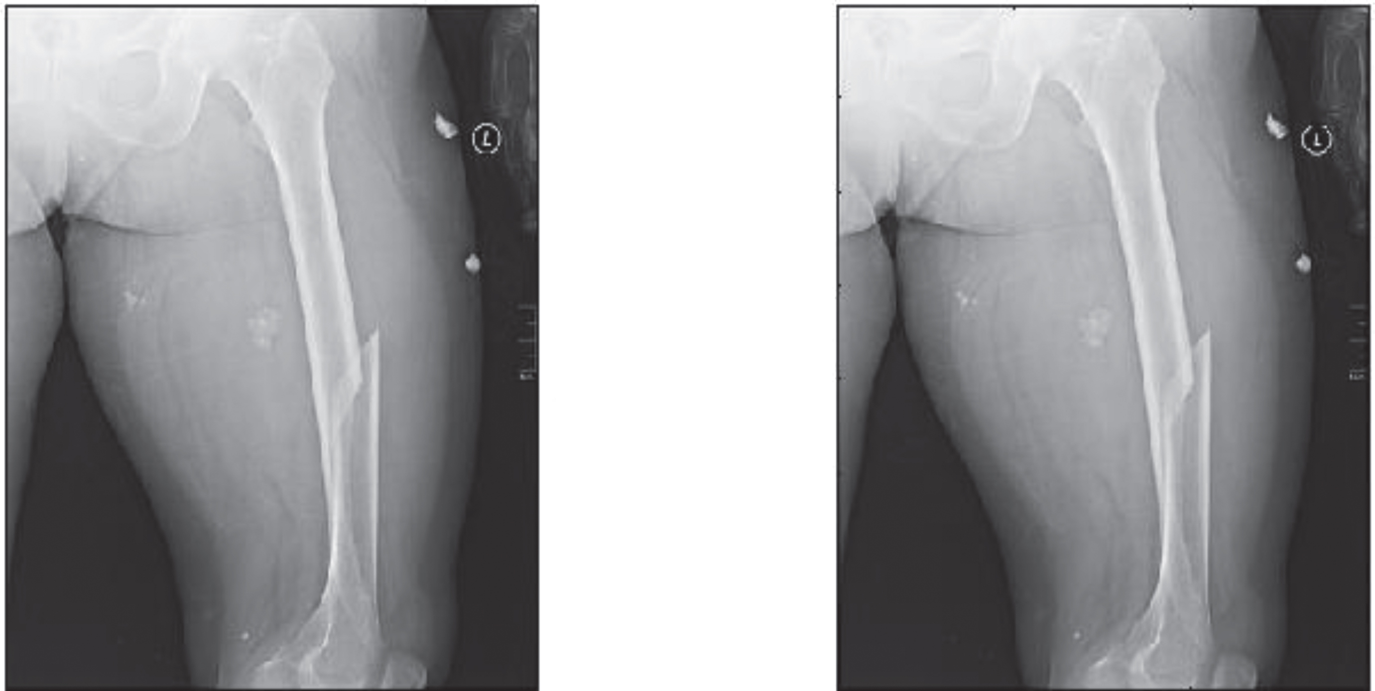
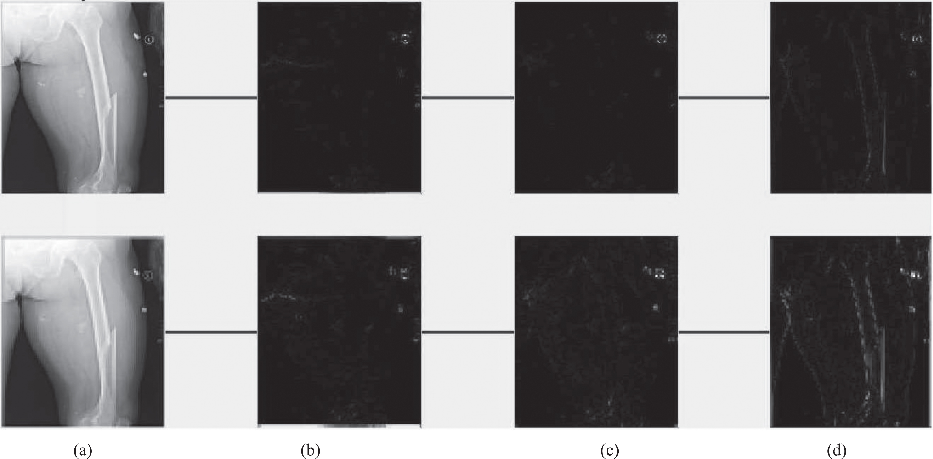
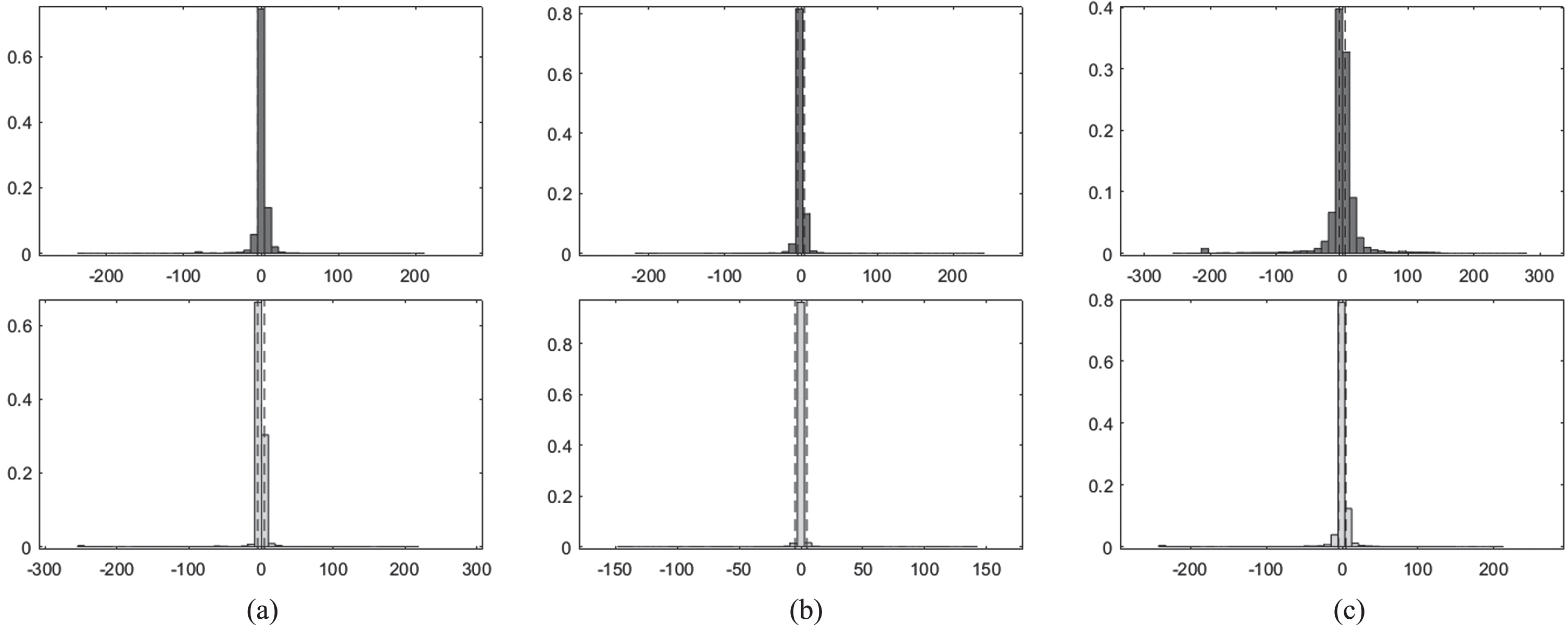
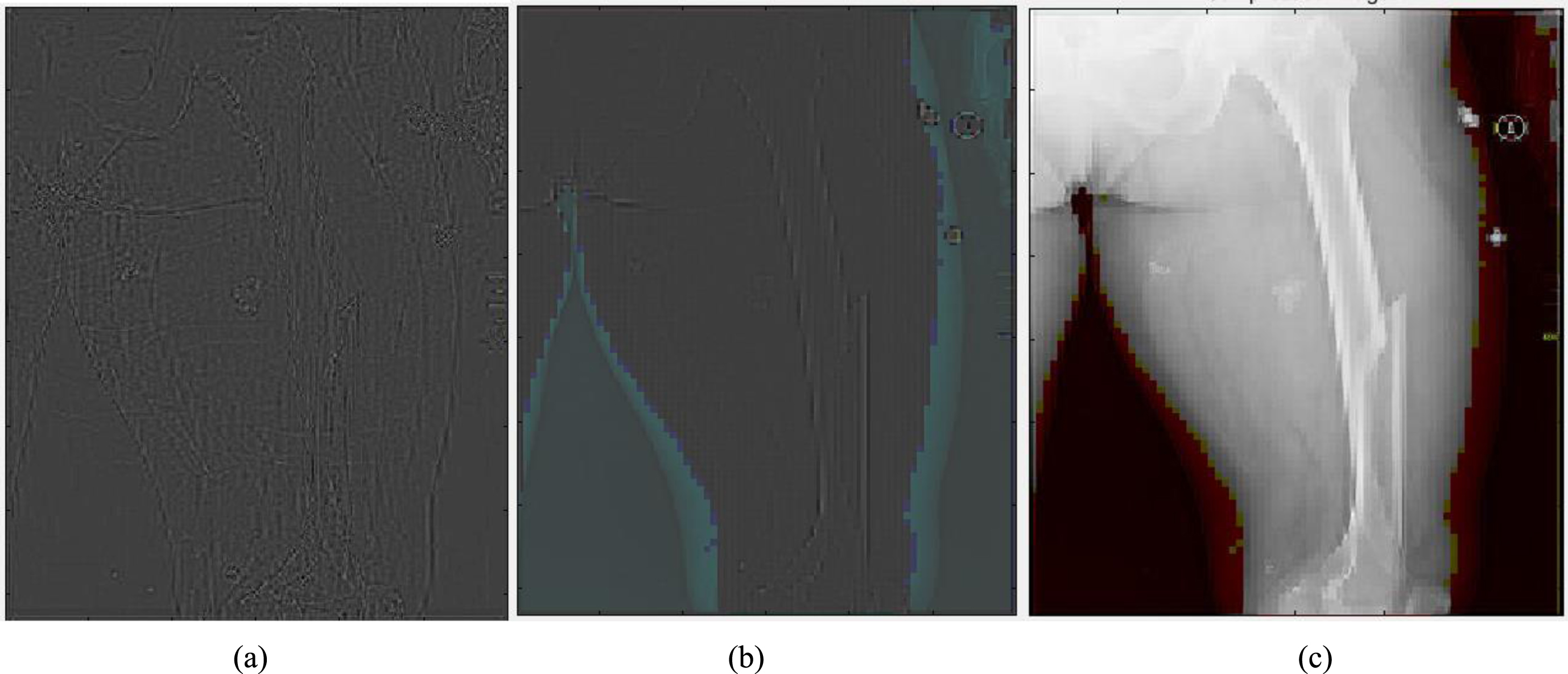
Figure 1 shows original Image (left), Synthesized image after feature point recognition (right) for set1. Figure 2 represents two rows, where Row 1 shows the proposed model output for 10 epochs –Set 1 (a) Feature Point Recognition (b) Deep-IRI architecture (c) CGAN based modelling (d) Learning-Based Injury Projection. The second row in Fig. 2 represents the proposed model output for 50 epochs (a) Feature Point Recognition (b) Deep-IRI architecture (c) CGAN based modelling (d) Learning-Based Injury Projection. Figure 3 shows histogram plots for Set 1 where Row 1 shows proposed model output for 10 epochs (a) Deep-IRI architecture (b) CGAN based modelling (c) Learning-Based Injury Projection and Row 2 shows proposed model output for 50 epochs (a) Deep-IRI architecture (b) CGAN based modelling (c) Learning-Based Injury Projection. Figure 4 shows the identification of injury region using proposed method in Set 1(a) Mask specific output (b) Proposed Patch-based discriminator output (c) Output of proposed generator network.

Fig. 1

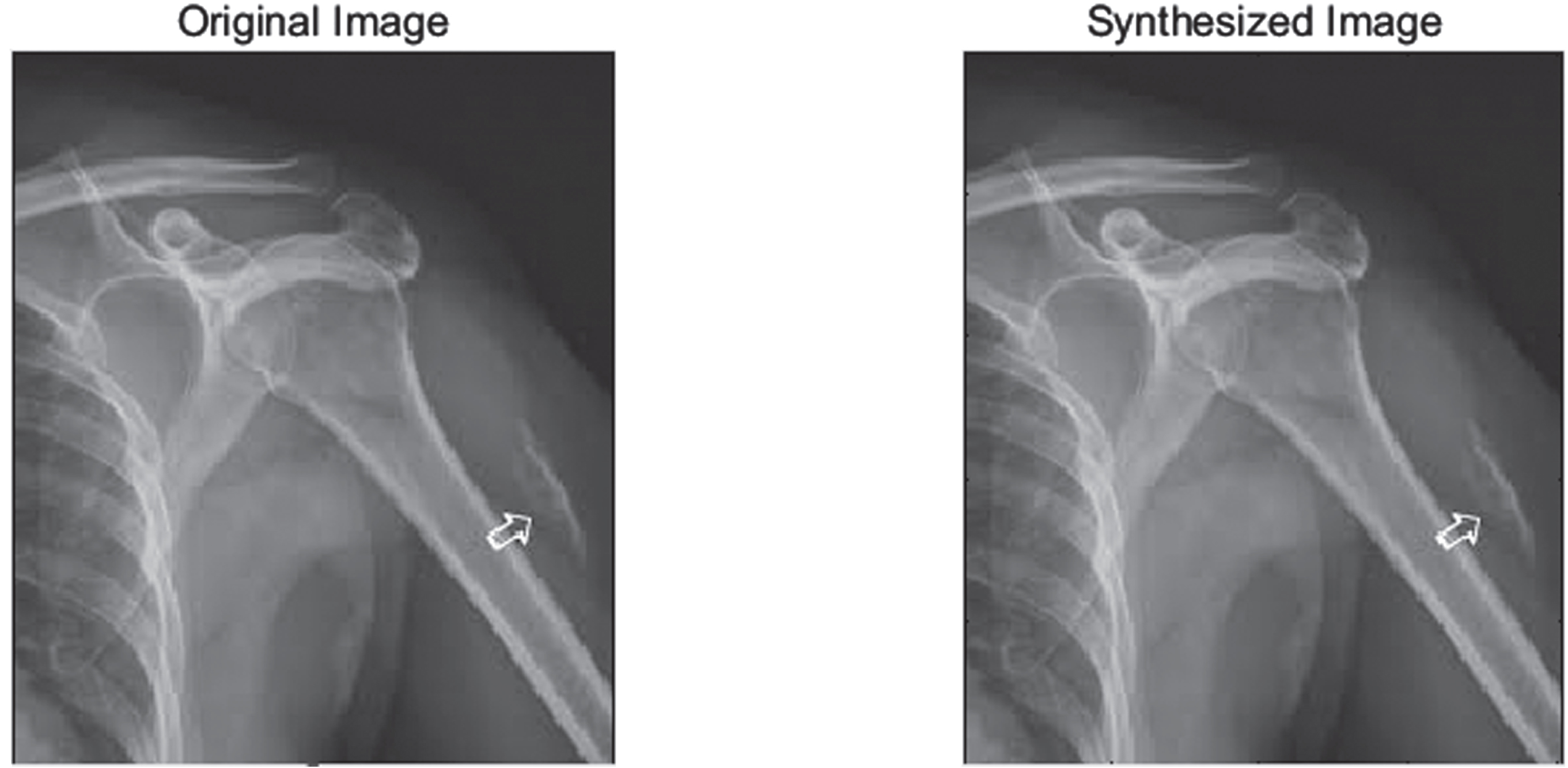
Original Image (left), Synthesized image after feature point recognition (right) - Set1.

Fig. 2

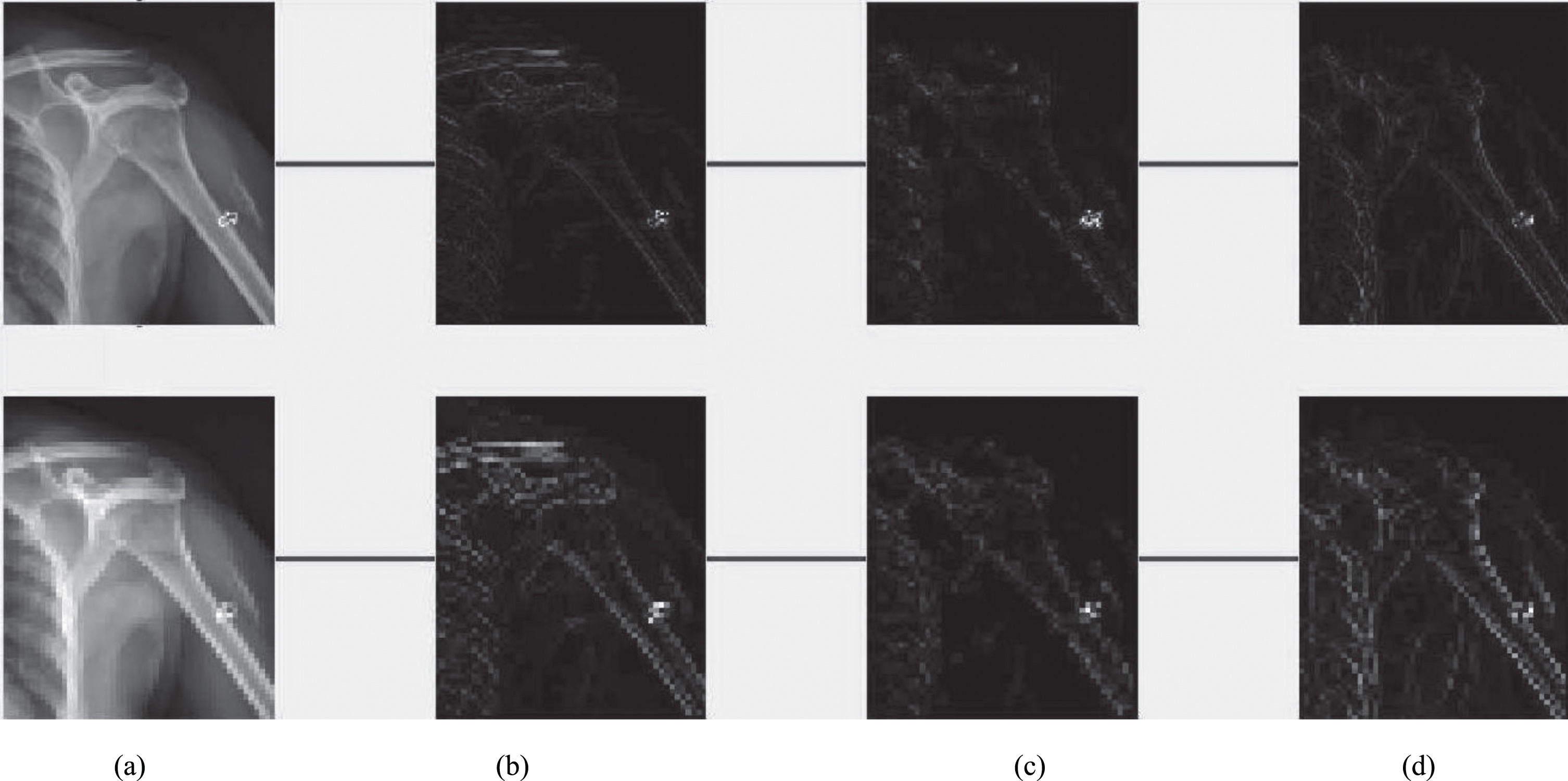
Row 1: Proposed model output for 10 epochs –Set 1 (a) Feature Point Recognition (b) Deep-IRI architecture (c) CGAN based modelling (d) Learning-Based Injury Projection. Row 2: Proposed model output for 50 epochs (a) Feature Point Recognition (b) Deep-IRI architecture (c) CGAN based modelling (d) Learning-Based Injury Projection.

Fig. 3

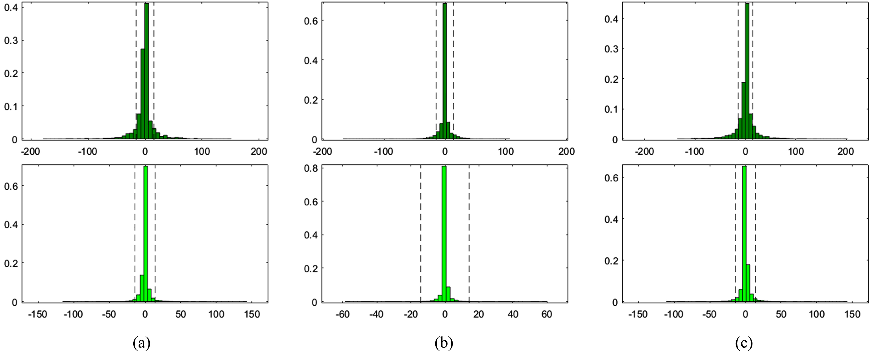
Histogram plots for Set 1- Row 1: Proposed model output for 10 epochs (a) Deep-IRI architecture (b) CGAN based modelling (c) Learning-Based Injury Projection. Row 2: Proposed model output for 50 epochs (a) Deep-IRI architecture (b) CGAN based modelling (c) Learning-Based Injury Projection.

Fig. 4

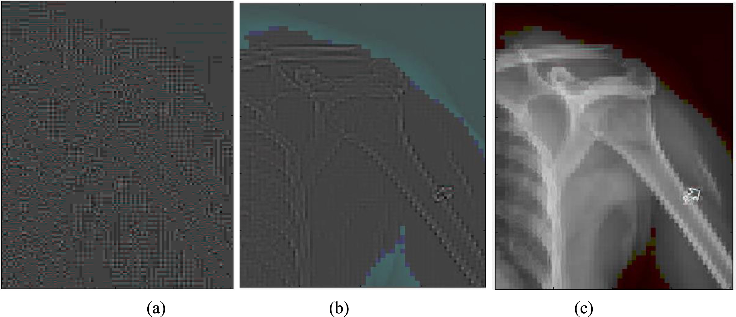
Identification of injury region using proposed method in Set 1(a) Mask specific output (b) Proposed Patch-based discriminator output (c) Output of proposed generator network.

It is observed that a more straightforward ray-based simulation would be enough for due to the mandatory nature of the completion training. Using zero padding helps ensure that the size of the network input and output are comparable. Additional genuine training data was included into this dataset. In addition, in order to balance the size of the network intake and output, In order to make the detection, zero padding was performed. Table 4 presents the comparison results of proposed method with state of art methods [17 –19]. Figure 5 shows original Image (left), Synthesized image after feature point recognition (right) for set2. Figure 6 represents two rows, where Row 1 shows the proposed model output for 10 epochs –Set 2 (a) Feature Point Recognition (b) Deep-IRI architecture (c) CGAN based modelling (d) Learning-Based Injury Projection. The second row in Fig. 6 represents the proposed model output for 50 epochs (a) Feature Point Recognition (b) Deep-IRI architecture (c) CGAN based modelling (d) Learning-Based Injury Projection. Figure 7 shows histogram plots for Set 2 where Row 1 shows proposed model output for 10 epochs (a) Deep-IRI architecture (b) CGAN based modelling (c) Learning-Based Injury Projection and Row 2 shows proposed model output for 50 epochs (a) Deep-IRI architecture (b) CGAN based modelling (c) Learning-Based Injury Projection. Figure 8 shows the identification of injury region using proposed method in Set 2(a) Mask specific output (b) Proposed Patch-based discriminator output (c) Output of proposed generator network.

Table 4

Comparison results of proposed method with state of art methods

	P. Rajpurkar, et al., 2017 [17]	A. F. M. Saif, et al., 2019 [18]	K. Teeyapan, 2021 [19]	Proposed method
Method used	DenseNet baseline model architecture	Capsule network architecture	EfficientNet network architecture	Feature Poitn recognition and GAN based DNN Architecture
Dataset used	MURA dataset [38]	MURA dataset [38]	MURA dataset [38]	MURA dataset [38]
Accuracy	0.929 (AUROC)	93.6% (maximum)	0.717 (Kappa Scoore)	94.9%

Fig. 5

Original Image (left), Synthesized image after feature point recognition (right) –Set2.

Fig. 6

Row 1: Proposed model output for 10 epochs –Set 2 (a) Feature Point Recognition (b) Deep-IRI architecture (c) CGAN based modelling (d) Learning-Based Injury Projection. Row 2: Proposed model output for 50 epochs (a) Feature Point Recognition (b) Deep-IRI architecture (c) CGAN based modelling (d) Learning-Based Injury Projection.

Fig. 7

Histogram plots for Set 2- Row 1: Proposed model output for 10 epochs (a) Deep-IRI architecture (b) CGAN based modelling (c) Learning-Based Injury Projection. Row 2: Proposed model output for 50 epochs (a) Deep-IRI architecture (b) CGAN based modelling (c) Learning-Based Injury Projection.

Fig. 8

Identification of injury region using proposed method in Set 2 (a) Mask specific output (b) Proposed Patch-based discriminator output (c) Output of proposed generator network.

During the training of the CGAN, there were 624 unique slices that contain considerable amounts of injury traces that were carefully recognised from the image. In addition to that, horizontal flips of this data were utilised as a data augmentation approach. This genuine information was used for transfer learning is exactly what was discussed before. FBP reconstructions were created, and a threshold mask was also implemented. Using a disk-shaped structuring element with a radius of 2 pixels and a resolution of 4 pixels respectively, to get a complete injury region. In order to get maximum performance from the CGAN network, the original GAN training approach [28] was used. The alternations between one gradient descending step on G and one step on D was carried out, with the one and only difference being that for the first iterations on D were performed for each epoch, with k = 1 as gradient descent iteration on G. Both sets of simulated data were run via stochastic descent gradient with a mini-batch size of 6. In the case of simulated data, the CGAN was trained for a total of 50 epochs using 50,000 training instances. The data enabling learning is used to be transferred from simulated data that was learned on the network. So, it is trained in the proposed neural network model for a total of 10–50 epochs. In addition to improving the efficiency of transfer learning, a model using already trained generator network G is also trained.

5 Conclusion

The proposed model is also subjected to an assessment to determine how effective it is, using the results of the experiment as the basis. In addition to qualitative comparisons, quantitative analysis based on the outcomes of the reconstruction was carried out using various performance metrics. These metrics were used in conjunction with the average peak signal to noise ratio. The approach that has been provided has been quite successful in maintaining the information on the boundaries of the objects and their regularity. After anything has been broken down into its component parts and arranged in a number of categories, having this information makes it much easier to be able to keep track of all of those parts. In addition to this, evaluate the efficacy of proposed models by doing work on the dataset while making use of X-ray images. These models were trained, and transfer learning was used throughout the process.

Footnotes

Acknowledgments

The author acknowledges the Deanship of Scientific Research, (Linyi University) for providing support for the publication of this research project.

Conflict of interest

The authors declare no conflict of interest.

Funding

This research received no external funding.

References

Almekinders

L.C.

, Muscles injuries and antiinflammatory treatment,110S, Med Sci Sports Exerc 23(suppl) (1991), 383.

Aronen

J.G.

, Garrick

J.G.

, Chronister

R.D.

and McDevitt

E.R.

, Quadriceps contusions: Clinical results of immediate immobilization in 120 degrees of knee flexion, Clin J Sport Med 16(5) (2006), 383–387.

Arrington

E.D.

and Miller

M.D.

, Skeletal muscle injuries, Orthop Clin North Am 26(3) (1995), 411–422.

Bedair

H.S.

, Karthikeyan

, Quintero

et al. Angiotensin II receptor blockade administered after injury improves muscle regeneration and decreases fibrosis in normal skeletal muscle, Am J Sports Med 36(8) (2008), 1548–1554.

Beiner

J.M.

and Jokl

, Muscle contusion injuries: Current treatment options, J Am Acad Ortho Surg 9(4) (2001), 227–237.

Zhou

, Hara

, Fujita

et al. Preliminary study for automated recognition of anatomical structure from torso CT images, Shanghai, China,, in Proc 27th Annu Conf Eng Medicine Biol (EMBC) (2005), 340.

Zhou

, Kamiya

, Hara

et al. Automated segmentation and recognition of abdominal wall muscles in X-ray torso CT images and its application in abdominal CAD, International Journal of Computer Assisted Radiology and Surgery 2(Supplement 1) (2007), 389–390.

Ekstrand

, Hägglund

and Waldén

, Epidemiology of muscle injuries in professional football (soccer), Am J Sports Med 39 (2011), 1226–232.

Elliott

M.C.

, Zarins

, Powell

J.W.

and Kenyon

C.D.

, Hamstring muscle strains in professional football players: A 10-year review, Am J Sports Med 39 (2011), 843–850.

10.

Mueller-Wohlfahrt

H.W.

, Haensel

, Mithoefer

et al. Terminology and classification of muscle injuries in sport: The Munich consensus statement, Br J Sports Med 47 (2013), 342–350.

11.

Pollock

, James

S.L.

, Lee

J.C.

and Chakraverty

, British athletics muscle injury classification: A new grading system, Br J Sports Med 48 (2014), 1347–1351.

12.

Valle

, Alentorn-Geli

, Tol

J.L.

et al. Muscle injuries in sports: A new evidence-informed and expert consensus-based classification with clinical application, Sports Med 47 (2017), 1241–1253.

13.

Balius

, Alomar

, Rodas

et al. The soleus muscle: MRI, anatomic and histologic findings in cadavers with clinical correlation of strain injury distribution, Skeletal Radiol 42 (2013), 521–530.

14.

Gillies

A.R.

and Lieber

R.L.

, Structure and function of the skeletal muscle extracellular matrix, Muscle Nerve 44 (2011), 318–331.

15.

Brukner

, Cook

J.L.

and Purdam

C.R.

, Does the intramuscular tendon act like a free tendon? Br J Sports Med 52 (2018), 1227–1228.

16.

Study Group of the Muscle and Tendon System from the Spanish Society of Sports Traumatology, A histoarchitectural approach to skeletal muscle injury. Searching for a common nomenclature, J Orthopaed J Sports Med 8(3) (2020), 2325967120909090.

17.

Rajpurkar

, Irvin

, Bagul

et al. MURA: Large dataset for abnormality detection in musculoskeletal radiographs,’ in Proc 1st Conf Med Imag Deep Learn (MIDL), 2017, pp. 1–10.

18.

Saif

A.F.M.

, Shahnaz

, Zhu

and Ahmad

M.O.

, Abnormality detection in musculoskeletal radiographs using capsule network, IEEE Access 7 (2019), 81494–81503.

19.

Teeyapan

Abnormality detection in musculoskeletal radiographs using EfficientNets, 2020 24th International Computer Science and Engineering Conference (ICSEC), Bangkok, Thailand, 2020, DOI: 10.1109/ICSEC51790.2020.9375275.

20.

Available at: https://orthoinfo.aaos.org/en/diseases–conditions/hamstring-muscle-injuries/.

21.

Isola

, Zhu

, Zhou

, Efros

A.A.

Image-to-image translation with conditional adversarial networks, in 2017 IEEE Conference on Computer Vision and Pattern Recognition (CVPR), 2017, pp. 5967–5976.

22.

Zhao

, Gallo

, Frosio

et al. Loss functions for image restoration with neural networks, IEEE Transactions on Computational Imaging 3(1) (2017), 47–57.

23.

Goodfellow

, Pouget-Abadie

, Mirza

et al. Generative adversarial nets, in Advances in 420 Neural Information Processing Systems, 2014, pp. 2672–2680.

24.

van Opbroek

Ikram

M.A.

Vernooij

M.W

de Bruijne

, Transfer learning improves supervised image segmentation across imaging protocols, IEEE Trans Med Imaging 34(5) (2015), 1018–1030.

25.

Shin

H.C.

, Roth

H.R.

, Gao

et al. Deep convolutional neural networks for computer-aided detection: CNN architectures, dataset characteristics and transfer learning, IEEE Trans Med Imaging 35(5) (2016), 1285–1298.

26.

, Xiong

, Yu

S.X.

, Lin

Unsupervised feature learning via non-parametric instance discrimination, in Proc IEEE/CVF Conf Comput Vis Pattern Recognit, 2018, pp. 3733–3742.

27.

Long

, Shelhamer

, Darrell

Fully convolutional networks for semantic segmentation, in Proceedings of the IEEE Conference on Computer Vision and Pattern Recognition, 2015, pp. 3431–3440.

28.

Mostayed

, Wee

, Zhou

Content-adaptive u-net architecture for medical image segmentation, in 2019 International Conference on Computational Science and Computational Intelligence (CSCI), Piscataway: IEEE; 2019, pp. 698–702.

29.

Luo

, Li

, Urtasun

, Zemel

Understanding the effective receptive field in deep convolutional neural networks, in Advances in Neural Information Processing Systems, 2016, pp. 4898–4906.

30.

Kayalibay

, Jensen

, van

CNN-based segmentation of medical imaging data, arXiv preprint, 2017, arXiv:1701.03056.

31.

, Chen

, Hu

, Yang

Understanding the disharmony between dropout and batch normalization by variance shift, arXiv preprint, 2018, arXiv:1801.05134.

32.

Deng

, Dong

, Socher

et al. Imagenet: A large-scale hierarchical image database, in Computer Vision and Pattern Recognition, IEEE, 2009, pp. 248–255.

33.

Yosinski

, Clune

, Bengio

, Lipson

How transferable are features in deep neural networks? in Advances in Neural Information Processing Systems, 2014, pp. 3320–3328.

34.

Pan

and Yang

, A survey on transfer learning, IEEE Transactions on Knowledge and Data Engineering 22(10) (2010), 1345–1359.

35.

Gutman

, Codella

N.C.F.

, Celebi

et al. Skin lesion analysis toward melanoma detection: A challenge at the International Symposium on Biomedical Imaging (ISBI) 2016, hosted by the International Skin Imaging Collaboration (ISIC), arXiv preprint, 2016, arXiv:1605.01397.

36.

Rodner

, Simon

, Brehm

et al. Fine-grained recognition datasets for biodiversity analysis, arXiv preprint, 2015, arXiv:1507.00913.

37.

Malmgren-Hansen

, Kusk

, Dall

et al. Improving SAR automatic target recognition models with transfer learning from simulated data, IEEE Geoscience and Remote Sensing Letters 14(9) (2017), 1484–1488.

38.

Available at: https://stanfordmlgroup.github.io/competitions/mura/.

Automated recognition of the major muscle injury in athletes on X-ray CT images 1