Sage Journals: Discover world-class research

Abstract

BACKGROUND:

Early diagnosis of breast cancer is crucial to perform effective therapy. Many medical imaging modalities including MRI, CT, and ultrasound are used to diagnose cancer.

OBJECTIVE:

This study aims to investigate feasibility of applying transfer learning techniques to train convoluted neural networks (CNNs) to automatically diagnose breast cancer via ultrasound images.

METHODS:

Transfer learning techniques helped CNNs recognise breast cancer in ultrasound images. Each model’s training and validation accuracies were assessed using the ultrasound image dataset. Ultrasound images educated and tested the models.

RESULTS:

MobileNet had the greatest accuracy during training and DenseNet121 during validation. Transfer learning algorithms can detect breast cancer in ultrasound images.

CONCLUSIONS:

Based on the results, transfer learning models may be useful for automated breast cancer diagnosis in ultrasound images. However, only a trained medical professional should diagnose cancer, and computational approaches should only be used to help make quick decisions.

Keywords

Breast cancer ultrasound imaging deep learning Convoluted Neural Networks image classification

1 Introduction

Cancer is a group of disorders typified by uncontrolled cell proliferation that may infiltrate and spread. A lump, unusual bleeding, prolonged cough, weight loss, and gastrointestinal changes may indicate cancer [1 –3]. Malignant tumours have anaplasia, invasiveness, and metastasis. Malignant tumours develop non-self-limitingly and invade adjacent tissues and metastasis [4]. Breast cancer kills women worldwide. After menopause, the risk of breast cancer decreases. 12% of American women will get breast cancer, and over 250,000 were diagnosed in 2017 [5, 6]. Steroid- and growth factor-induced breast cell mitogenesis requires D-type and E-type cyclins to govern the G1-to-S phase transition. During cell cycle development. Primary breast cancer often overexpresses cyclins D1 and E1 [8].

Machine learning is growing quickly. Understanding its surroundings, machine learning mimics human intelligence. Machine learning is useful in the era of large data [9]. Deep learning allows computer systems with numerous processing layers to learn new data representations, improving object recognition, object detection, medication development, genomics, and other fields [11, 12]. Deep learning has been used to medicine development, genetics, and other fields. One of the most often used deep neural networks is the CNN, which can handle millions of parameters with less processing [13, 14]. This research endeavour used US breast cancer and unaffected tissue pictures to teach a CNN to identify breast cancer.

ML has substantially improved several medical imaging procedures [15, 16]. Deep learning (DL) is a valuable subset of machine learning (ML) since CNNs were initially developed for image processing [17]. Machine learning and deep learning are being used to picture categorization, object identification, and segmentation [17 –19]. The US might benefit from creating new diagnostic assistance technologies. Classification approximates picture label [20]. CNN classifies US breast cancer photos as benign or malignant. CNN added a matching layer to classify breast mass [21]. Support vector machines, very general purpose (VGG), and recurrent neural networks (ResNet) identified breast US pictures [22]. Object detection may quickly recognise picture landmarks. VGG and ResNet [23] classified US pictures and detected lesions. Three US-collected deep learning models were tested for breast cancer lesion detection. Segmentation improves measurements and target structures. A U-net segmentation method was developed for ultrasonography breast mass assessment. Compared to segmentation, object detection provides more information [24] and saves money on labelling data and training networks [25, 26]. For the reasons above, object detection is used to identify breast disease lesions in US images. This ML tools speed up radiologist diagnosis without compromising sensitivity and specificity [27].

Medical imaging uses ultrasound (US). It is portable, radiation-free, and cheaper than magnetic resonance and computed tomography [28]. This article gathered US breast cancer pictures (benign and malignant) and unaffected tissues. These photos trained CNN to anticipate breast cancer.

Recent developments in the field of medical imaging research have focused on the use of machine learning technology to the process of identifying and grading cancerous tissue in ultrasound pictures obtained from tumours. It has been shown that algorithms based on machine learning, and in particular deep learning, are capable of reliably identifying and categorising tumours in medical imaging, including ultrasound scans.

The topic of cancer is one area where there is promise for the use of machine learning technologies for the identification and grading of cancer in ultrasound pictures. The precise diagnosis and grading of prostate cancer is essential for efficient treatment and management of this kind of cancer, which is the second most frequent form of cancer in men globally. The current techniques for diagnosing and grading prostate cancer entail intrusive procedures such as biopsies, which may cause the patient to experience discomfort and even suffering. Machine learning algorithms might correctly identify and grade prostate cancer from ultrasound imaging. This non-invasive biopsy approach is painless. Machine learning on ultrasound images may help diagnose other cancers. Mammography and ultrasound are used to test for breast cancer, but their high false-positive rate is a drawback. The application of machine learning algorithms to reliably identify between benign and malignant breast tumours in ultrasound pictures has the potential to increase the accuracy of breast cancer screening while also reducing the amount of needless biopsies.

The use of machine learning technology to the task of identifying and grading cancerous tissue in ultrasound pictures of tumours has the potential to completely change the way cancer is diagnosed and treated. It is a non-invasive and less expensive alternative to the conventional procedures, while at the same time increasing accuracy and decreasing the amount of further testing that is required. However, further research and development is required to assure the safety and reliability of machine learning algorithms in clinical practise and to optimise machine learning algorithms for the application in question.

Thus, early identification of breast cancer is crucial to effective therapy. Cancer diagnosis uses MRI, CT, and ultrasound studies. This research work uses transfer learning algorithms to train convoluted neural networks (CNNs) to automatically identify breast cancer on ultrasound pictures.

Transfer learning models trained CNNs have been used in this work to identify breast cancer in ultrasound pictures. The models’ training and validation accuracies were assessed using ultrasound pictures. MobileNet and DenseNet121 achieved the greatest training and validation accuracy in the research. Transfer learning methods identify breast cancer on ultrasound pictures.

2 Methods

This section delineates the protocols that must be adhered to in conducting disease detection tests for the project. The process flow for selecting the optimal model is presented in Fig. 1, while Fig. 2 depicts how the model predicts disease from raw data during the training and validation stages by adjusting hyper-parameters. The following paragraphs provide a succinct overview of each of the blocks presented in the diagrams and their relevance in this study.

Fig. 1

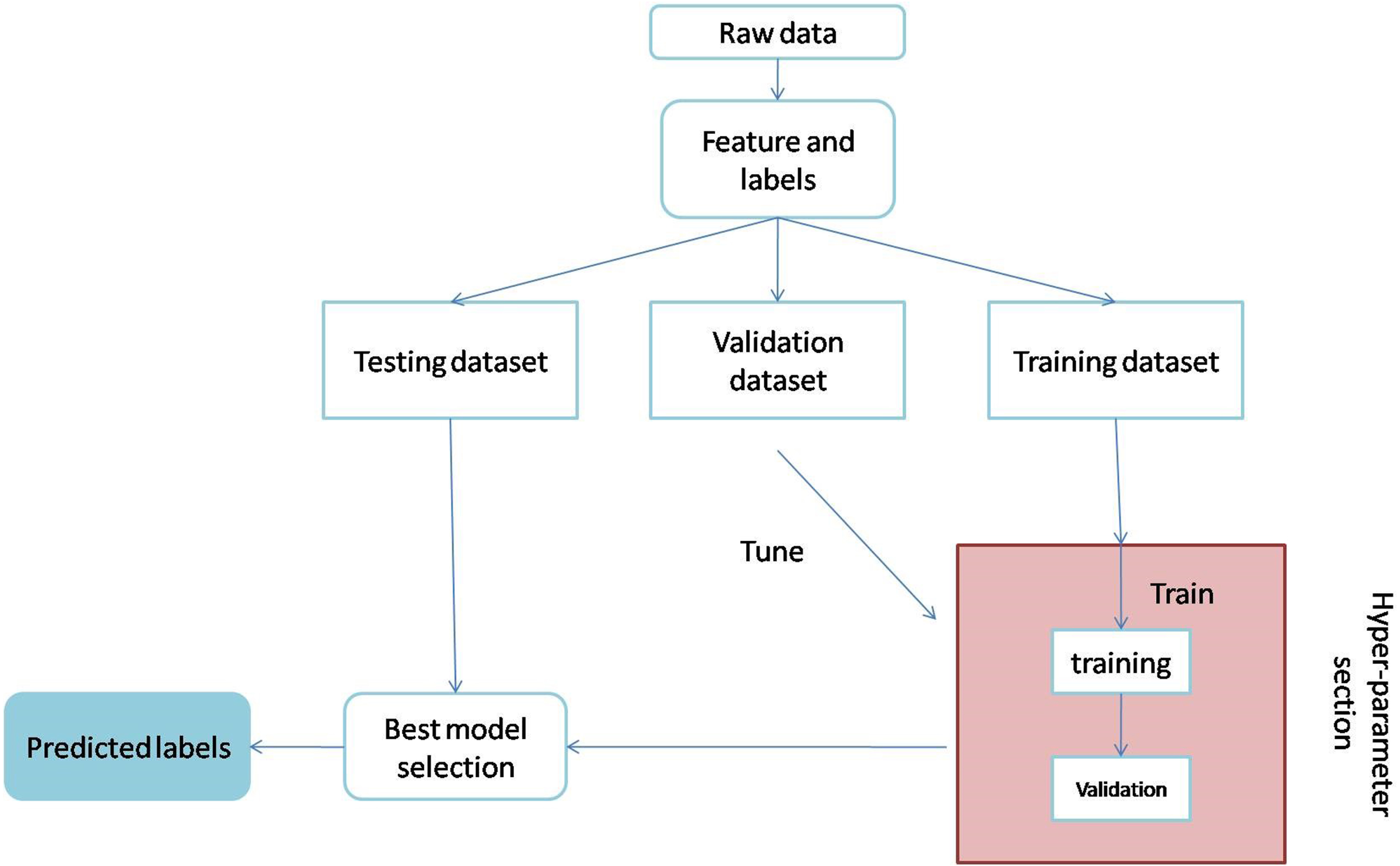
Process flow for selection of best modelling.

Fig. 2

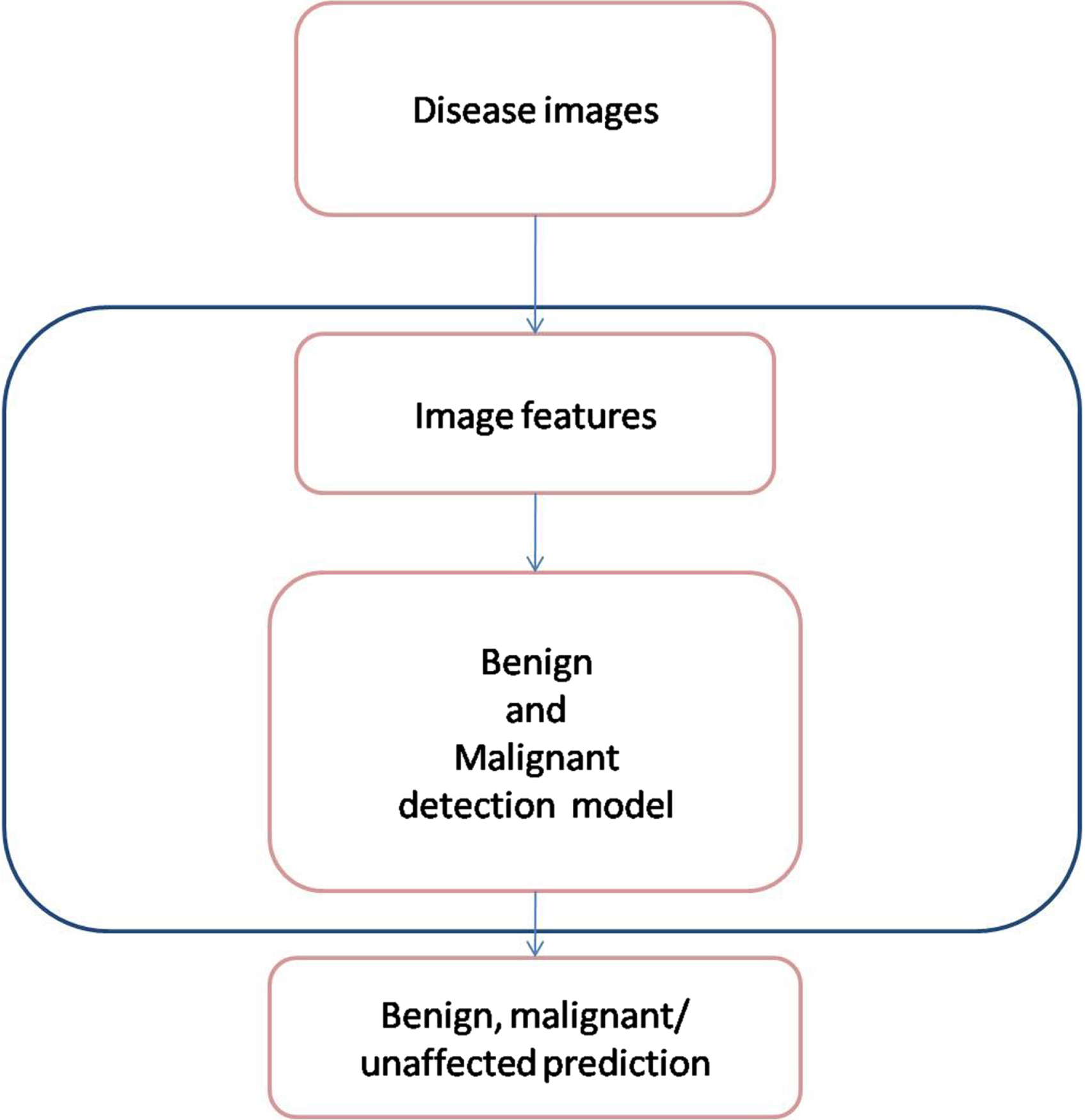
Classification of cancer type by the best model.

2.1 Dataset collection

This study obtained ultrasound images of breast cancer and normal breast tissues from two different sources. The first source contained over 437 benign breast cancer ultrasound images, 210 malignant breast cancer ultrasound images, and 133 unaffected tissue images [29]. The second source contained over 200 benign and 200 normal breast ultrasound images [30]. A total of 637 benign, 410 malignant and over 133 unaffected tissue images were used in this study.

2.2 Image pre-processing

A single dataset containing benign, malignant and unaffected tissues was created by combining multiple datasets as mentioned previously. As ultrasound images are of different sizes, OpenCV was used to resize the image to 224×224 pixels. The US photos were then processed to eliminate the backdrop. The dataset is loaded and transformed into an array using the NumPy library for training purposes.

2.3 Overview of the proposed modelling

Multiple transfer learning models are evaluated to determine the best model for detecting breast cancer in ultrasound images. The explanation for each of these models is provided below.

2.3.1 MobileNet

MobileNet is a model that is both effective and lightweight in its design. It is based on a straightforward concept that constructs low-weight deep neural networks by the use of depth-wise separable convolutions. The inclusion of only two simple global hyper-parameters achieves an effective equilibrium between accuracy and latency. These hyper-parameters make it easier for the model builder to choose a model size that is suitable for their application in light of the restrictions posed by the challenge. Extensive testing on resource and accuracy tradeoffs are reported, and the results show high performance in comparison to other popular ImageNet classification models [31].

2.3.2 MobileNetV2

The MobileNetV2 architecture is constructed on an inverted residual structure, which means that the input and output of the residual block are narrow bottleneck layers. This is in contrast to the usual residual models, which make use of expanded representations in both the input and output. In order to filter features in the intermediate expansion layer, MobileNetV2 takes use of low weight depthwise convolutions. MobileNetV2 enhances the overall performance of mobile models over a broad spectrum of activities and benchmarks, regardless of the size of the model [32].

2.3.3 DenseNet121

The fundamental justification for using DenseNet121 is that it solves the vanishing gradient problem, improves feature reuse, and reduces parameter usage, all of which are beneficial for training deep learning models. DenseNet121 is effective in the diagnosis of disorders with medical imaging. DenseNet121 would be driven by linking each layer to every layer below it to optimize the architecture flow. This method allows CNN to decide based on all levels rather than just one final layer [33].

2.3.4 DenseNet169

DenseNet169 is a convolutional neural network structure with a dense block. All the preceding sub-input block’s feature maps are concatenated and used like the following feature map. This extended relationship benefits the resolution of vanishing gradient problems and parameter number reduction [34, 35].

2.3.5 DenseNet 201

DenseNet201 is a brand-new DNN architecture for healthcare applications. DNNs have been accelerated by using specialized accelerators such as GPUs. Nonetheless, GPUs are susceptible to transitory effects and other reliability risks, which can jeopardize the accuracy of DNN models [36].

2.3.6 NASNetMobile

NASNet is a scalable Convolutional Neural Network architecture that was constructed via the use of neural architecture search. It is composed of basic building blocks (cells) that have been modified by the use of reinforcement learning. NASNetMobile is a mobile version that has 564 million multiply accumulates, 5.3 million parameters, and 12 cells [37, 38].

2.3.7 VGG16

Malware categorization using the 16-layer DNN offered by Visual Geometry Group (VGG16). Using the convolution layer of VGG16 pre-trained on the ImageNet dataset, we extract the filter activation maps (also known as bottleneck features) via transfer learning [39].

2.3.8 VGG19

VGG-19 convolutional neural network with a densely connected classifier that has been tuned. We study the transfer learning method, in which we use knowledge from a model trained on a different task because of a lack of data [40].

All models are initiated with weight = “imagenet,” include top = False, and input shape = (224, 224, 3). A Flatten () layer is followed by 1024 hidden dense layers and a “relu,” a rectified linear activation function that directly produces a positive insert with an input dimension of 512. A 0.7 dropout factor was used. After dropout, 512 hidden dense layers with a “relu” (rectified linear activation function) were added. Then 256 hidden dense layers were added with “relu” function. Following a 0.5 dropout, 128 hidden dense layers with “relu” function were added. There is another 0.4 dropout was applied. Further, then buried dense layers were added.

2.4 Evaluation Metrics

The models are assessed on the basis of several performance metrics stated below.

2.4.1 Confusion Matrix

The confusion matrix best illustrates the model’s performance. Specificity, sensitivity, accuracy, and precision are calculated using confusion matrices. Confusion matrices simplify comparing True Negatives, False Negatives, True Positives, and False Positives [41].

2.4.2 Accuracy

Accuracy is the ratio of the total of correctly classified samples to the sample size. It is a diagonal measure that ignores the rows and columns of the confusion matrix. Sokal and Michener first defined it as a “matching coefficient,” a similarity measure among two individuals with a series of binary attributes [42]. $Accuracy = \frac{(TP + TN)}{(TP + TN + FP + FN)}$ (1)

2.4.3 Precision

Precision is the probability of the presence of a sample, given a projected presence. It is the proportion of true positives to all positive cases [43]. $Pr ecision = \frac{TP}{(TP + FP)}$ (2)

2.4.4 F1-Score

F1-score, a synthetic one-dimensional indicator, is crucial for evaluating natural language or information retrieval systems. F measures accuracy and sensitivity harmonically. Researchers are now directly raising the F1-score to change system settings [44].

The MobileNet and DenseNet121 models were tested on a particular dataset as part of a classification or detection job. When compared to the other models that were tested, the MobileNet and DenseNet121 models obtained a high level of accuracy throughout the training and validation stages of the test. Both MobileNet and DenseNet121 are examples of models of convolutional neural networks (CNNs), which have been shown to be successful in a broad variety of computer vision applications. MobileNet and DenseNet121 both include MobileNet. DenseNet121 is a dense convolutional network that has shown great accuracy on image classification tests, while MobileNet was developed expressly for mobile and embedded vision applications. During the training phase, the models are presented with a collection of labelled training data, which enables them to acquire knowledge and make necessary adjustments to their weights and biases. During the validation phase, the model’s hyperparameters are fine-tuned and its performance is evaluated using an additional set of data that was not included during the training phase. It is quite probable that throughout these stages, the MobileNet and DenseNet121 models were able to extract significant characteristics from the input data and produce correct predictions, which resulted in strong performance on the task for which they were tested. Both MobileNet and DenseNet121 are successful deep learning models for a range of computer vision tasks, and they have shown high accuracy in a number of applications. In general, MobileNet and DenseNet121 are quite similar to one another.

Machine learning feature selection and optimisation often employ parametric analysis. This method optimises an algorithm’s parameters. Parametric analysis can optimise feature selection and algorithm selection for machine learning algorithms for feature augmentation. Radiomics examination of medical pictures may extract texture, contrast, and intensity. To identify medical issues, these traits are analysed using machine learning algorithms. The model is trained and assessed using various parameter values throughout optimisation. The algorithm, characteristics, and hyperparameters may be parameter values. Accuracy, precision, and recall are used to assess the model. Parametric analysis helps machine learning find the best features and algorithms for a job. Machine learning practitioners may increase model correctness and efficiency by altering parametric analysis parameters. The terms “accuracy,” “precision,” “recall,” “F1 score,” and “area under the curve” (AUC) of the receiver operating characteristic (ROC) curve are all examples of common assessment metrics.

3 Results and discussion

This study used different pre-trained models, namely DenseNet121, DenseNet169, DenseNet 201, MobileNetV2, MobileNet, VGG16, VGG19 and NASNetMobile to analyze ultrasound images of breast cancer at different stages, namely benign, malignant and normal tissues. The dataset contains 1180 images were divided into training, validation and test sets with a percentage ratio of 6:3:1 respectively and resized into 224×224 using OpenCV. The pre-trained models were maintained at a minimum learning rate and retained at 1e-5 under the “Adam” optimizer, with a decay rate of up to 1e-3/epoch. The process is carried out for 500 epochs with a batch size of 32.

As can be seen in Fig. 3, the confusion matrix shows accuracy both classes when put through their respective tests. A confusion matrix is constructed from the results of prediction attempts made on a classification issue. Count values are what are used in order to describe the number of correct and incorrect predictions for each category. This causes confusion whenever it makes predictions, which is why it serves as the key to the confusion matrix. Figure 4 refers the ROC curve. ROC curves are used to evaluate binary classification models in machine learning. The ROC curve compares TPR and FPR across classification levels. AUC, the area under the receiver operating characteristic curve, is used to evaluate model performance. A higher AUC implies better performance.

Fig. 3

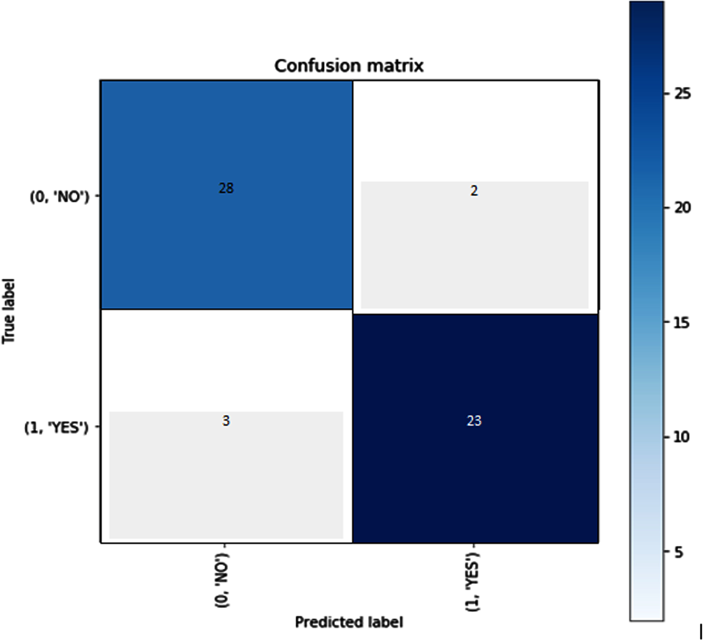
Confusion matrix.

Fig. 4

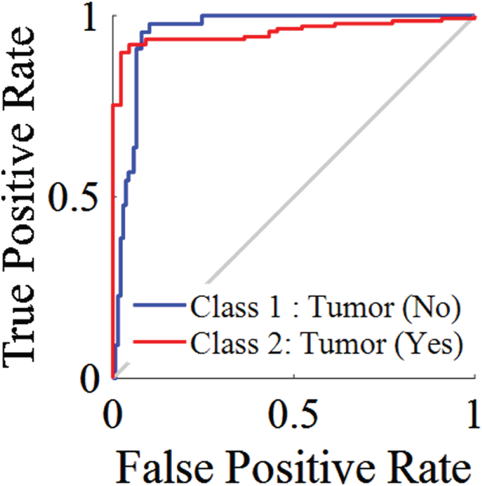
ROC Curve.

In order to determine how well a machine learning algorithm is doing, evaluation metrics are used in parametric analyses of its many aspects. These analyses are carried out in order to evaluate the effectiveness of the model. These metrics provide a quantitative assessment of how well the model has internalised the lessons imparted by the data.

The terms “accuracy,” “precision,” “recall,” “F1 score,” and “area under the curve” (AUC) of the receiver operating characteristic (ROC) curve are all examples of common assessment metrics. These metrics may be used to assess the performance of the model in relation to a variety of criteria, including true positives, true negatives, false positives, and false negatives.

When the training and validation dataset is small or homogenous, VGG16 and VGG19 may learn the same features and attain the same accuracy. Due to the dataset’s simplicity, VGG16’s linearized accuracy graph may have plateaued early in training. Learning rate, batch size, and optimizer may affect validation accuracy and accuracy graph form. These factors may have favoured VGG16 and VGG19 equally, resulting in equivalent graph accuracy and form. VGG16 and VGG19 may be overfitting the dataset and performing similarly on the validation set despite poor generalisation. Due to overfitting, VGG16’s linearized accuracy graph shows limited generalisation. Therefore, VGG16’s linearized accuracy graph and equivalent validation accuracy.

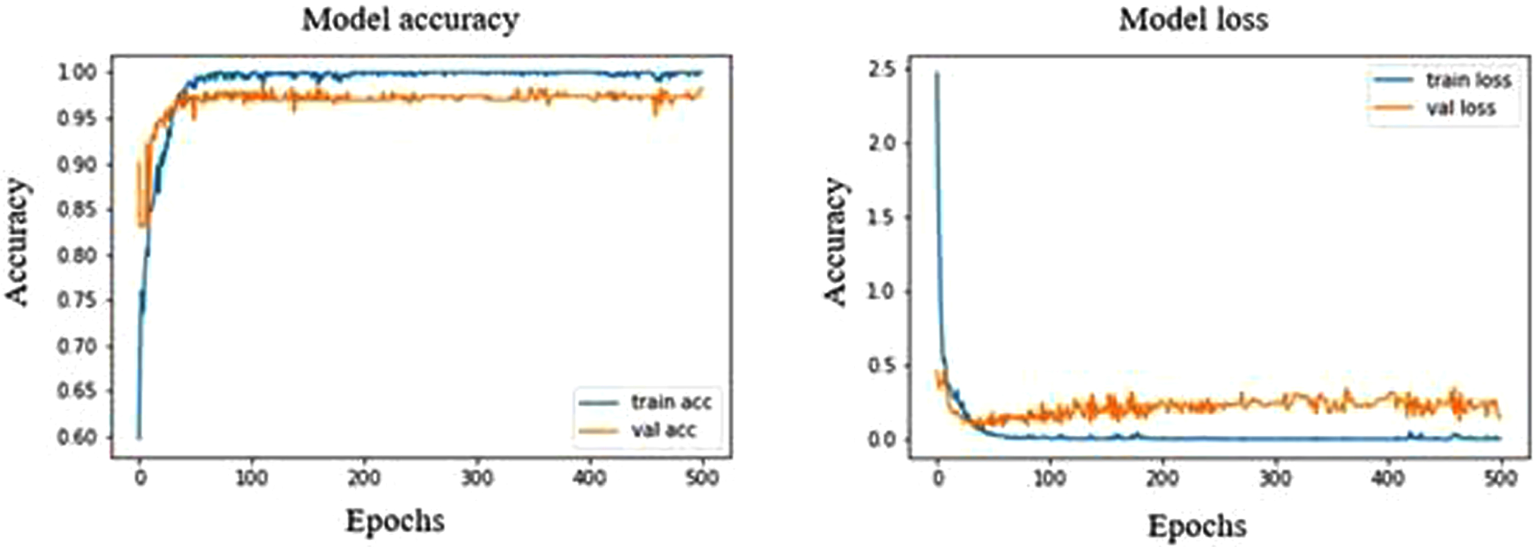
In DenseNet121, Epoch 373 and 496 have shown a high validation accuracy of 64.31% with corresponding validation loss of 27.88% and 33.58%, respectively and the training accuracy and loss was found to be 95.48% and 11.4%, respectively. In performance metrics, the accuracy and sensitivity of normal ultrasound images were high among other stages of breast cancer, indicating that the model is capable of recognizing the normal ultrasound images at a high rate. At epoch 10, the model shows an overfit strongly throughout the process in Fig. 5. This model has shown malignant with precision, recall and F1 scores of 7%, 50% and 12%, respectively. As for normal and benign, the precision, recall and F1 score are 97%, 71%, 82% and 71%, 97%, 82%, respectively.

Fig. 5

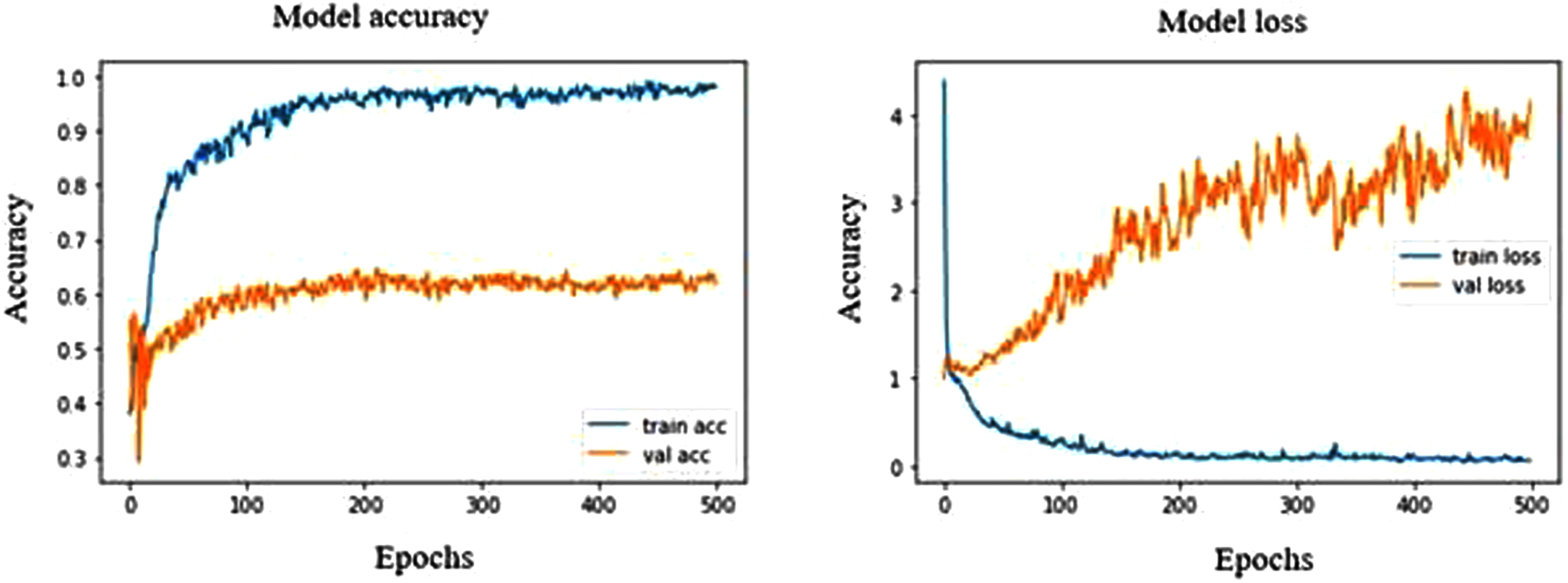
Model accuracy and loss plot of DenseNet121.

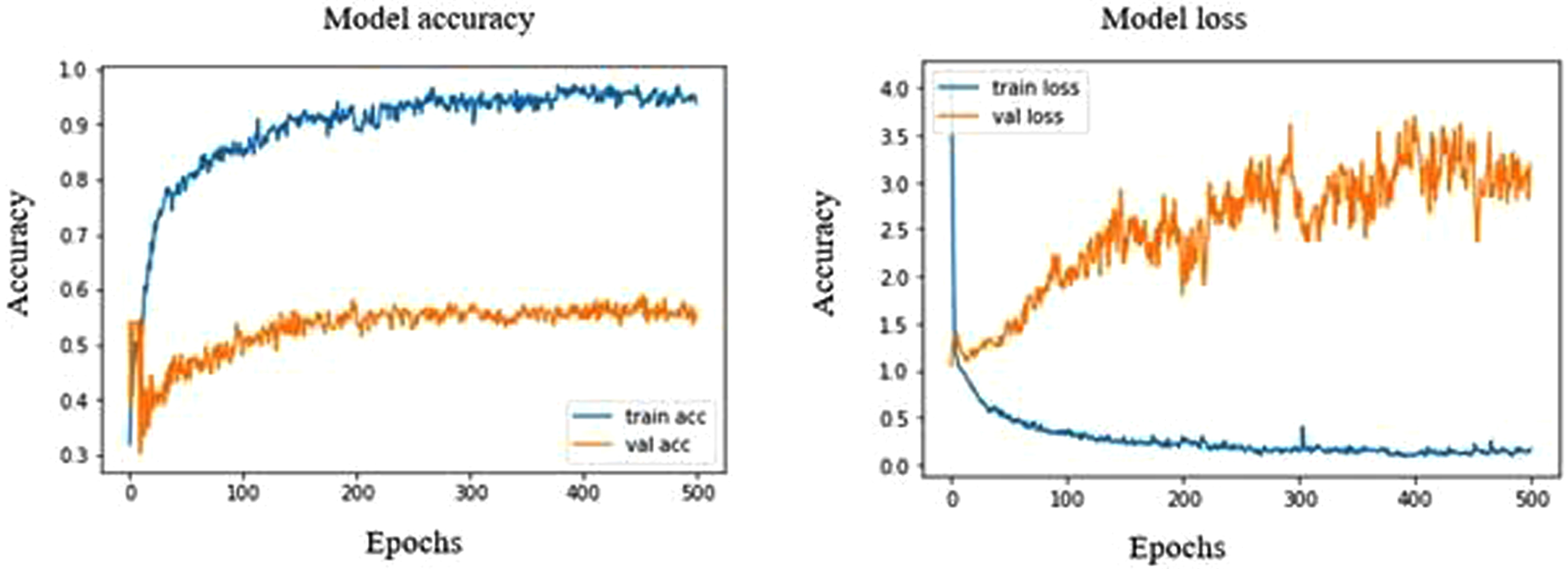
The highest validation accuracy in DenseNet169 was found to be 64.19% at both epoch 361 and 472, with a validation loss of 43.63% and 56.43%, respectively. The model has shown high sensitivity towards normal ultrasound images with a rate of 95.31%. From Fig. 6, we can observe that the validation accuracy shows fluctuation with a range of 50% to 60%, whereas the training accuracy extends up to a rate of 100%. This high fluctuation results in a strong over-fitting model with malignant showing a precision, recall and F1 score of 21%, 50% and 30%, respectively. As for normal and benign, the precision, recall and F1 score are 95%, 69%, 80% and 51%, 88%, 65%, respectively.

Fig. 6

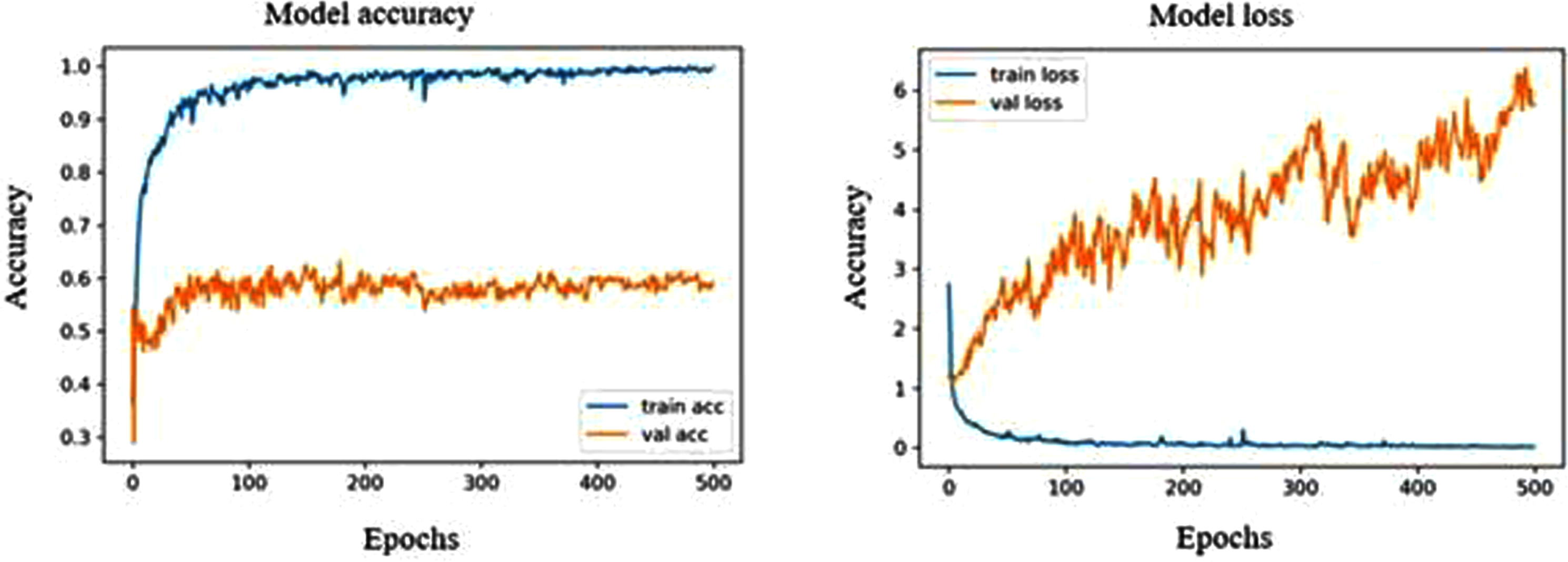
Model accuracy and loss plot of DenseNet169.

The DenseNet201 model shows a strong overfit in the accuracy and loss graph, as shown in Fig. 7. The validation accuracy remains stagnant between 50% to 60% and has shown high fluctuation throughout the process. The validation accuracy at epoch 229 is found to be 60.06% with a corresponding validation loss of 275.91%, which is the highest validation accuracy seen in this model with normal ultrasound images possessing a sensitivity of 98.43%, which shows that this model is a high capability to differentiate normal breast tissues from the tumorous tissues. The precision, recall and F1 score of the normal 98%,74% and 85%, whereas in the case of benign and malignant, it is found to be 61%, 100%, 76% and 57%, 89%, 70%, respectively.

Fig. 7

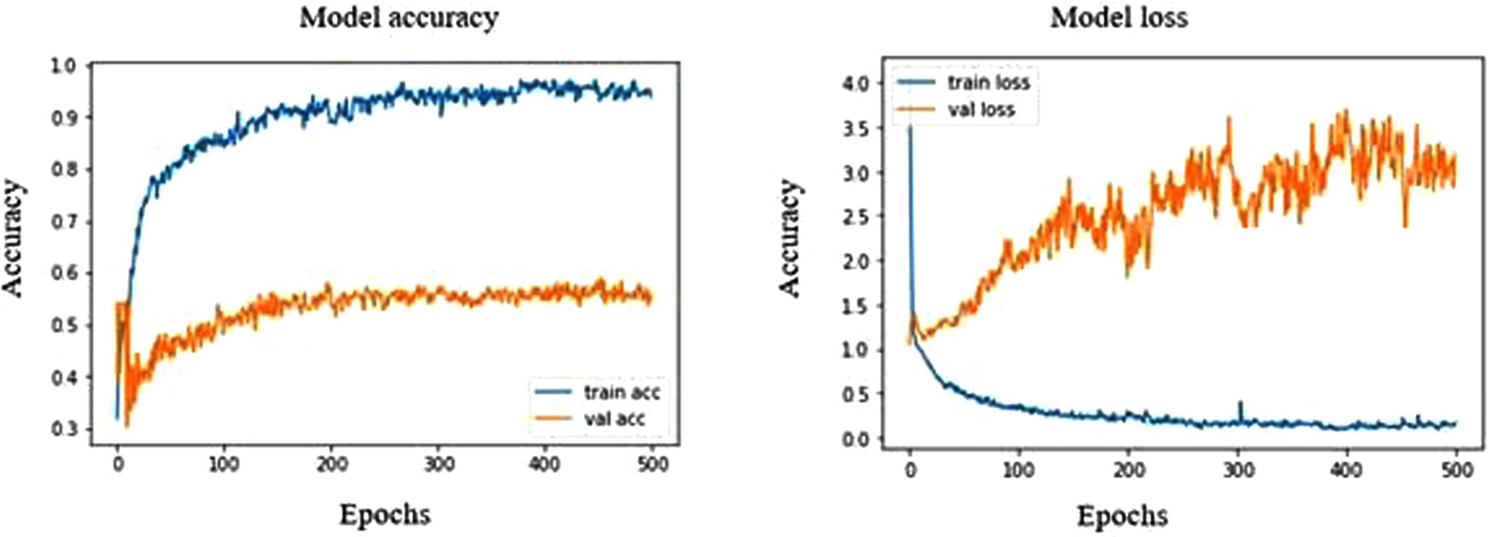
Model accuracy and loss plot of DenseNet201.

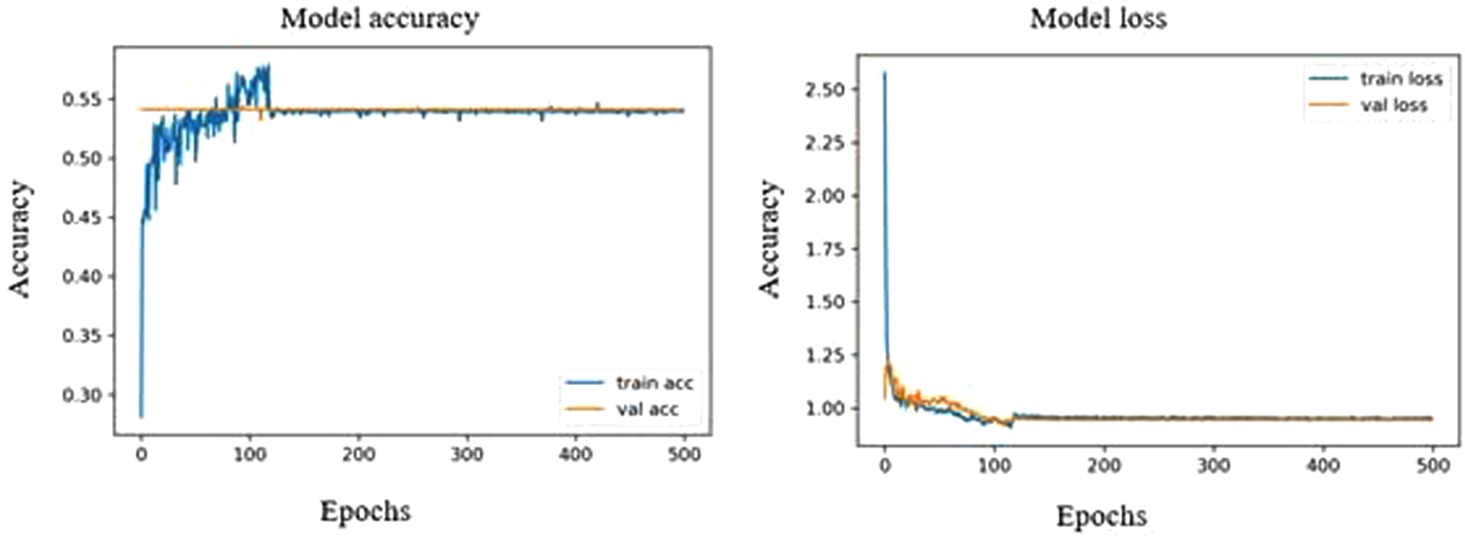
The pre-trained MobileNet model showed the highest validation accuracy of 53.36% at both 297 and 483 epochs. The corresponding validation loss was in the closer range of about 55.85% and 55.35%. The precision, recall and F1 score of the normal 97%,70% and 81%, whereas in the case of benign and malignant, it is found to be 29%, 80%,42% and 56%, 92%, 70%, respectively. From Fig. 8, we can see that the model over fits strongly with a sensitivity of 96.87% towards normal ultrasound images. At the same time, the highest validation accuracy of MobileNetV2 model is 49.29% which is comparatively low under MobileNet model. However, from Fig. 9, we can see that the MobileNetV2 model shows an optimal fitting with a sensitivity of 95.31% for normal images. The precision, recall and F1 score of malignant and benign were 14%, 50%, 22% and 49%, 95%, 65%, respectively.

Fig. 8

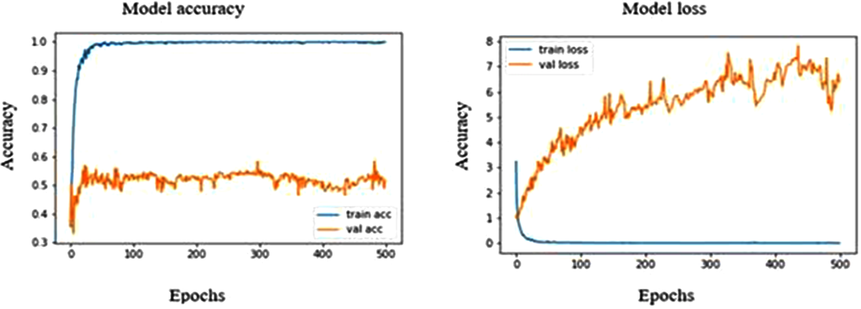
Model accuracy and loss plot of MobileNet.

Fig. 9

Model accuracy and loss plot of MobileNetV2.

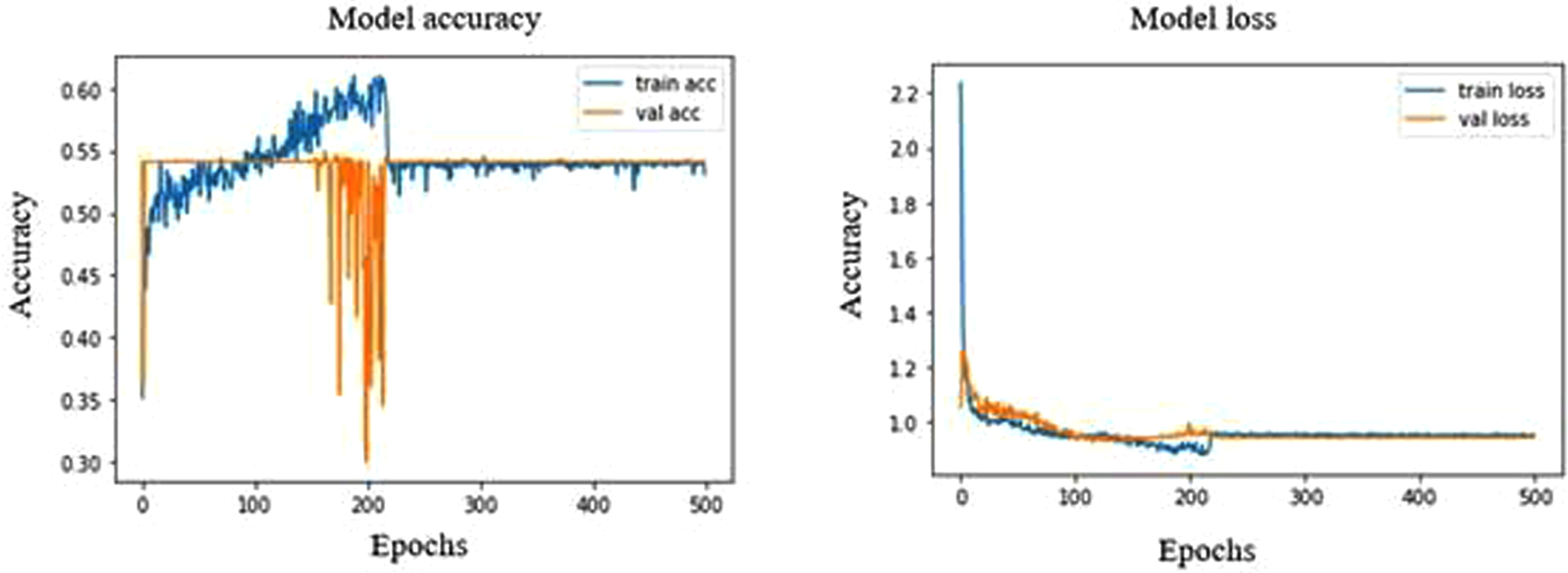
NASNetMobile model shows a validation accuracy of 58.92%, which is almost similar to that of MobileNet model. It strongly overfits the accuracy graph (Fig. 10) with a sensitivity of 92.18% for normal ultrasound images. The NASNetMobile has a precision, recall, F1 score of 63%, 81%, 71% and 21%, 60%, 32% for benign and malignant respectively, whereas normal images possess 92%, 72% and 81% respectively.

Fig. 10

Model accuracy and loss plot of NASNetMobile.

Both VGG16 and VGG19 showed the same validation accuracy of 54.11%, where the accuracy graph of VGG16 is linearized, and the accuracy graph of VGG19 deviates slightly at a range of 150 to 220 epochs (Fig. 11 and Fig. 12). Both VGG16 and VGG19 could only identify normal ultrasound images with a sensitivity of 100%. The precision, recall, and F1 scores share the same value for VGG16 and VGG19 in normal tissues, about 100%, 54%, and 70%, respectively.

Fig. 11

Model accuracy and loss plot of VGG16.

Fig. 12

Model accuracy and loss plot of VGG19.

Among the eight pre-trained models, the DenseNet121 shows the highest validation accuracy of 64.31% over the other models. MobileNet shows a training accuracy of 100%, which is the highest of all models. Out of all the pre-trained models, DenseNet121, DenseNet201, and MobileNetV2 showed a higher specificity of 99.04% in malignant ultrasound images, whereas DenseNet169, MobileNetV2 and NASNetMobile showed a closer specificity. The normal ultrasound images possessed the highest F1 scores when trained using the densenet201 model. Similarly, the normal images trained using densenet121, densenet169, MobileNet and NASNet showed a closer F1 score.

Latif et al., 2020 have built CNN models to detect and classify breast cancer. Their results indicate an accuracy of about 88% was obtained when using the CNN classifier [45]. Vesal et al., 2018 used pre-trained networks like AlexNet, GoogleNet, and ResNet to classify breast cancer and have an accuracy of about 85% [46]. Tanaka et al., 2019 built a CNN-based CAD system to classify breast cancer ultrasound images. The sensitivity specificity and AUC were over 95% [47]. Musad et al., 2021 have used the pre-trained CNN models like DenseNet201, ResNet50, and VGG16 using different optimizers to classify cancer images and got an accuracy of 100% [48]. Gómez-Flores et al., 2020 have used four CNN-based semantic segmentation models and eight pre-trained CNN architectures for the cancer image classification. ResNet50 showed the best segmentation performance with an F1 score exceeding 90% [49]. Vasile et al., 2018 have classified ultrasound images of thyroid disorders using pre-trained models showed a promising result with an overall sensitivity of 95% specificity of 98% and accuracy of about 97% exceedingly over 95% [50]. Deepak et al., 2021 have classified brain tumours with MRI images and showed a good performance with very few datasets. They showed a good specificity, recall, sensitivity of over 95% each [51]. Brinker et al., 2019 have used pre-trained AlexNet models to classify skin cancer and obtained an accuracy of about 93% for melanoma and non-melanoma, similarly an accuracy of 73% in classifying atypical melanomas [52]. Deepak et al., 2018 adopted pre-trained Xception, Inception v3, ResNet-50, VGG16, and MobileNet for the classification of brain tumour with a testing accuracy of about 97% and F1 scores and validation accuracy exceeding 90% [53].

4 Conclusion

Breast cancer is a disease that poses a significant threat to the lives of young women. Early detection and treatment are essential in reducing the mortality associated with this disease. Despite the widespread use of artificial neural networks for object classification and detection in various image processing applications, their utilization in the field of medical diagnosis remains limited. In light of this, the current study aimed to evaluate the effectiveness of different ImageNet models, including DenseNet121, DenseNet169, DenseNet201, MobileNetV2, MobileNet, VGG16, VGG19, and NASNetMobile, in the automated detection of malignant tumors in ultrasound images of the breast. Both MobileNet and DenseNet121 exhibited good accuracy during the training and validation phases. These results indicate the need for further experimentation with larger datasets to improve the performance of the models.

Author Contributions

Conceptualization, L.Z. and J.Z.; methodology, R.X.; software, J.Z.; validation, L.Z; formal analysis, R.X.; investigation, L.Z. and R.X; resources, J.Z; data curation, R.X., and L.Z.; writing— original draft preparation, J.Z.; writing— review and editing, L.Z.; visualization, J.Z.; supervision, R.X., and L.Z.; project administration, J.Z., and R.X.;. All authors have read and agreed to the published version of the manuscript.

Conflicts of interest

The authors declare that they have no conflicts of interest.

Data availability statement

The data used to support the findings of this study are included within the article.

Funding statement

There are no funds available for this research.

References

W.H. Organization, WHO guidelines for the pharmacological and radiotherapeutic management of cancer pain in adults and adolescents, 2018.

Dvorak

H.F.

, Tumors: wounds that do not heal, New England Journal of Medicine 315 (1986), 1650–1659.

Issah

, Maree

J.E.

and Mwinituo

P.P.

, Expressions of cervical cancer-related signs and symptoms, European Journal of Oncology Nursing 15 (2011), 67–72.

Wilkins

E.M.

, Clinical practice of the dental hygienist, Lea & Febiger Philadelphia, 1976.

Waks

A.G.

and Winer

E.P.

, Breast cancer treatment: a review, JAMA 321 (2019), 288–300.

Key

T.J.

, Verkasalo

P.K.

and Banks

, Epidemiology of breast cancer, The Lancet Oncology 2 (2001), 133–140.

Cowin

, Rowlands

T.M.

and Hatsell

S.J.

, Cadherins and catenins in breast cancer, Current Opinion in Cell Biology 17 (2005), 499–508.

Sutherland

R.L.

and Musgrove

E.A.

, Cyclins and breast cancer, Journal of Mammary Gland Biology and Neoplasia 9 (2004), 95–104.

El Naqa

and Murphy

M.J.

, What is machine learning?, in: Machine Learning in Radiation Oncology”, Springer, (2015), pp. 3–11.

10.

Jordan

M.I.

and Mitchell

T.M.

, Machine learning: Trends, perspectives, and prospects, Science 349 (2015), 255–260.

11.

LeCun

, Bengio

and Hinton

, Deep learning, Nature 521 (2015), 436–444.

12.

Rusk

, Deep learning, Nature Methods 13 (2016), 35–35.

13.

Chauhan

, Ghanshala

K.K.

and Joshi

R.C.

, Convolutional neural network (CNN) for image detection and recognition, In 2018 First International Conference on Secure Cyber Computing and Communication (ICSCCC), IEEE, (2018), pp. 278–282.

14.

Albawi

, Mohammed

T.A.

and Al-Zawi

, Understanding of a convolutional neural network, In 2017 International Conference on Engineering and Technology (ICET), IEEE, (2017), pp. 1–6.

15.

Komatsu

, Sakai

, Dozen

, et al., Towards clinical application of artificial intelligence in ultrasound imaging, Biomedicines 9 (2021), 720.

16.

Takahashi

, Takahashi

, Kinoshita

, et al., Fine-tuning approach for segmentation of gliomas in brain magnetic resonance images with a machine learning method to normalize image differences among facilities, Cancers 13 (2021), 1415–.

17.

LeCun

, Bengio

and Hinton

, Deep Learning, Nature 521 (2015), 436–444.

18.

Zhao

Z.Q.

, Zheng

and Wu

, Object detection with deep learning: A review, IEEE Trans Neural Networks Learn Syst 30 (2019), 3212–3232.

19.

Lateef

and Ruichek

, Survey on semantic segmentation using deep learning techniques, Neurocomputing 338 (2019), 321–348.

20.

Han

, Kang

H.K.

, Jeong

J.Y.

, et al., A Deep learning framework for supporting the classification of breast lesions in ultrasound images, Phys Med Biol 62 (2017), 7714.

21.

Byra

, Galperin

, Ojeda-Fournier

, et al., Breast mass classification in sonography with transfer learning using a deep convolutional neural network and color conversion, Med Phys 46 (2019), 746–755.

22.

Antropova

, Huynh

B.Q.

and Giger

M.L.

, A deep feature fusion methodology for breast cancer diagnosis demonstrated on three imaging modality datasets, Med Phys 44 (2017), 5162–5171.

23.

Zhu

Y.C.

, AlZoubi

, Jassim

, et al., A generic deep learning framework to classify thyroid and breast lesions in ultrasound images, Ultrasonics 110 (2021), 106300.

24.

Kumar

, Webb

J.M.

, Gregory

, et al., Automated and real-time segmentation of suspicious breast masses using convolutional neural network, PloS One 13 (2018), e0195816.

25.

Alom

M.Z.

, Taha

T.M.

, Yakopcic

, et al., A state-of-the-art survey on deep learning theory and architectures, Electronics 8 (2019), 292.

26.

Hariharan

, Arbeláez

, Girshick

and Malik

, Simultaneous detection and segmentation, In: European Conference on Computer Vision. Zürich, Switzerland: Springer (2014), pp. 297–312.

27.

Yap

M.H.

, Pons

, Martí

, et al., Automated breast ultrasound lesions detection using convolutional neural networks, IEEE J Biomed Health Inf 22 (2017), 1218–1226.

28.

Chan

and Perlas

, Basics of ultrasound imaging, InAtlas of Ultrasound-Guided Procedures in Interventional Pain Management, Springer, (2011), pp. 13–19.

29.

Al-Dhabyani

, Gomaa

, Khaled

and Fahmy

, Dataset of breast ultrasound images, Data in Brief 28 (2020), 104863.

30.

Badawy

S.M.

, Mohamed

A.E.-N.A.

, Hefnawy

A.A.

, et al., Automatic semantic segmentation of breast tumors in ultrasound images based on combining fuzzy logic and deep learning— A feasibility study, PloS One 16 (2021), e0251899.

31.

Howard

A.G.

, Zhu

, Chen

, et al., Mobilenets: Efficient convolutional neural networks for mobile vision applications, ArXiv Preprint ArXiv:1704.04861, 2017.

32.

Sandler

, Howard

, Zhu

, et al., Mobilenetv2: Inverted residuals and linear bottlenecks, In Proceedings of the IEEE Conference on Computer Vision and Pattern Recognition, (2018), pp 4510–4520.

33.

Roy

, Kiral-Kornek

and Harrer

, ChronoNet: a deep recurrent neural network for abnormal EEG identification, In Conference on Artificial Intelligence in Medicine in Europe, Springer, (2016), pp. 47–56.

34.

Suh

Y.J.

, Jung

and Cho

B.-J.

, Automated breast cancer detection in digital mammograms of various densities via deep learning, Journal of Personalized Medicine 10 (2020), 211.

35.

Huang

, Liu

, Van Der Maaten

and Weinberger

K.Q.

, Densely connected convolutional networks, In Proceedings of the IEEE Conference on Computer Vision and Pattern Recognition, (2017), pp. 4700–4708.

36.

Adam

, Mohamed

I.I.

and Ibrahim

, A selective mitigation technique of soft errors for DNN models used in healthcare applications: Densenet201 case study, IEEE Access 9 (2021), 65803–65823.

37.

Zoph

, Vasudevan

, Shlens

and Le

Q.V.

, Learning transferable architectures for scalable image recognition, In Proceedings of the IEEE Conference on Computer Vision and Pattern Recognition (2018), pp. 8697–8710.

38.

Saxen

, Werner

, Handrich

, et al., Face attribute detection with MobileNetV2 and NasNet-Mobile, In 2019 11th International Symposium on Image and Signal Processing and Analysis (ISPA), IEEE, (2019), pp. 176–180.

39.

Rezende

, Ruppert

, Carvalho

, et al., Malicious software classification using VGG16 deep neural network’s bottleneck features, In Information Technology-New Generations, Springer, (2018), pp. 51–59.

40.

Simonyan

and Zisserman

, Very deep convolutional networks for large-scale image recognition, ArXiv Preprint ArXiv, 1409.1556, 2014.

41.

Hasan

M.K.

, Tanha

, Amin

M.R.

, et al., Cataract disease detection by using transfer learning-based intelligent methods, Computational and Mathematical Methods in Medicine (2021), 7666356.

42.

Goodall

D.W.

, The distribution of the matching coefficient, Biometrics (1967), 647–656.

43.

Sofaer

H.R.

, Hoeting

J.A.

and Jarnevich

C.S.

, The area under the precision-recall curve as a performance metric for rare binary events, Methods in Ecology and Evolution 10 (2019), 565–577.

44.

Huang

, Xu

, Wang

and Silamu

, Maximum F1-score discriminative training criterion for automatic mispronunciation detection, IEEE/ACM Transactions on Audio, Speech, and Language Processing 23 (2015), 787–797.

45.

Latif

, Butt

M.O.

, Al Anezi

F.Y.

and Alghazo

, Ultrasound image despeckling and detection of breast cancer using deep CNN, In 2020 RIVF International Conference on Computing and Communication Technologies (RIVF), IEEE (2020), pp. 1–5.

46.

Vesal

, Ravikumar

, Davari

, et al., Classification of breast cancer histology images using transfer learning, In International Conference Image Analysis and Recognition, Springer, (2018), pp. 812–819.

47.

Tanaka

, Chiu

S.W.

, Watanabe

, et al., Computer-aided diagnosis system for breast ultrasound images using deep learning, Physics in Medicine & Biology 64 (2019), 235013.

48.

Masud

, Hossain

M.S.

, Alhumyani

, et al., Pre-trained convolutional neural networks for breast cancer detection using ultrasound images, ACM Transactions on Internet Technology (TOIT) 21 (2021), 1–17.

49.

Gómez-Flores

and de Albuquerque Pereira

W.C.

, A comparative study of pre-trained convolutional neural networks for semantic segmentation of breast tumors in ultrasound, Computers in Biology and Medicine 126 (2020), 104036.

50.

Seetha

and Raja

S.S.

, Brain tumor classification using convolutional neural networks, Biomedical & Pharmacology Journal 11 (2018), 1457.

51.

Vasile

C.M.

, Udriştoiu

A.L.

, Ghenea

A.E.

, et al., Intelligent diagnosis of thyroid ultrasound imaging using an ensemble of deep learning methods, Medicina 57 (2021), 395.

52.

Deepak

and Ameer

P.M.

, Brain tumor classification using deep CNN features via transfer learning, Computers in Biology and Medicine 111 (2019), 103345.

53.

Brinker

T.J.

, Hekler

, Utikal

J.S.

, et al., Skin cancer classification using convolutional neural networks: systematic review, Journal of Medical Internet Research 20 (2018), e11936.

Learning technology for detection and grading of cancer tissue using tumour ultrasound images 1

Abstract

BACKGROUND:

OBJECTIVE:

METHODS:

RESULTS:

CONCLUSIONS:

Keywords

1 Introduction

2 Methods

2.2 Image pre-processing

2.3 Overview of the proposed modelling

2.3.1 MobileNet

2.3.2 MobileNetV2

2.3.3 DenseNet121

2.3.4 DenseNet169

2.3.5 DenseNet 201

2.3.6 NASNetMobile

2.3.7 VGG16

2.3.8 VGG19

2.4 Evaluation Metrics

2.4.1 Confusion Matrix

2.4.2 Accuracy

3 Results and discussion

Author Contributions

Conflicts of interest

Data availability statement

Funding statement

References