
Abstract
AMIE+ is a state-of-the-art algorithm for learning rules from RDF knowledge graphs (KGs). Based on association rule learning, AMIE+ constituted a breakthrough in terms of speed on large data compared to the previous generation of ILP-based systems. In this paper we present several algorithmic extensions to AMIE+, which make it faster, and the support for data pre-processing and model post-processing, which provides a more comprehensive coverage of the linked data mining process than does the original AMIE+ implementation. The main contributions are related to performance improvement: (1) the top-k approach, which addresses the problem of combinatorial explosion often resulting from a hand-set minimum support threshold, (2) a grammar that allows to define fine-grained patterns reducing the size of the search space, and (3) a faster projection binding reducing the number of repetitive calculations. Other enhancements include the possibility to mine across multiple graphs, the support for discretization of continuous values, and the selection of the most representative rules using proven rule pruning and clustering algorithms. Benchmarks show reductions in mining time of up to several orders of magnitude compared to AMIE+. An open-source implementation is available under the name RDFRules at
Keywords
Introduction
Finding interesting interpretable patterns in data is a frequently performed task in data science workflows. Software for finding association rules, as a specific form of patterns, is present in nearly all data mining software bundles. These implementations are based on the Apriori algorithm [2] or its successors. While very fast, these algorithms are severely constrained with respect to the shape of analyzed data – only single tables or transactional data are accepted. Algorithms for logical rule mining developed within the scope of Inductive Logical Programming (ILP) do not have these restrictions, but they typically require negative examples and do not scale to larger knowledge graphs (KGs) [20].
Commonly used open KGs, such as Wikidata [55], DBpedia [5], and YAGO [51], are published in RDF [4] as sets of triples – statements in the form of binary relationships. Most of these RDF KGs1
Also “RDF Knowledge Graph”, which is a term used in related research (e.g., [3,26]) to denote a KG formed as a collection of statements in the RDF format.
The current state-of-the-art approach for rule mining from RDF KGs is AMIE+ [20]. AMIE+ combines the main principles that make association rule learning fast with the expressivity of ILP systems. AMIE+ mines Horn rules, which have the form of implication and consist of one atomic formula (or simply atom) on the right side, called head, and conjunction of atoms on the left side, called body:
Since all atoms are binary, we use an infix notation, which is more readable here than the prefix (first-order logic) notation used in ILP. We also distinguish variables with a question mark, and the Internationalized Resource Identifiers (IRIs) with angle brackets. See Section 3 for more details.
In our view, AMIE+ constitutes a big leap forward in learning rules from KGs, similar in magnitude to what the invention of Apriori meant for rule learning from transactional data. However, AMIE+ also shares some notable limitations with the original Apriori algorithm. Decades of research in association rule learning and frequent itemset mining continuously show how difficult it is for users to constraint the search space so that meaningful rules are generated, and combinatorial explosion is avoided. In the presented work, we address these limitations by drawing inspiration from techniques proven in rule mining from transactional databases. The extensions to AMIE+ introduced in this paper include a top-k approach, which can circumvent the need for the user manually tuning the support threshold, fine-grained search space restrictions, avoidance of some repetitive calculations, and the ability to discretize values in numerical literals.
Together, these optimisations substantially reduce the large search space of potential rules that have to be checked. All the aforementioned approaches have been implemented within the RDFRules framework and evaluated in comparison with the original AMIE+ implementation. Additionally, this article describes two post-processing approaches – rule clustering and pruning – adopted for RDF KGs. These techniques are necessary to address the high number of rules that are typically on the output of rule mining.
The scope of functionality of RDFRules is inspired by the widely used arules framework [23] for rule learning from tabular data. Similarly to arules, RDFRules covers the complete data mining process, including data pre-processing (support for numerical attributes), various mining settings (fine-grained patterns and measures of significance), and post-processing of mining results (rule clustering, pruning, filtering and sorting).
We provide benchmarks demonstrating the benefits of the proposed performance enhancements. For example, for mining rules with constants – which are an essential element of association rules mined from tabular data – the AMIE+ algorithm can take hours (or days), but the presented approach has a more than an order of magnitude shorter mining time on YAGO and DBpedia. Similarly, the top-k approach can provide a more than ten times shorter mining time compared to the standard approach supported by AMIE+ when all rules conforming to the user-set minimum support threshold are first mined and then filtered. We also show that our implementation scales better than AMIE+ when additional CPU cores are added.
This paper is organised as follows. Section 2 provides a broader overview of related work. A digest of the AMIE+ approach is ranged as Section 3. Section 4 presents a list of limitations of AMIE+, providing the motivation for our work. The proposed approach is described in Section 5. Section 6 briefly describes its reference implementation. The results of the evaluation are presented in Section 7. The conclusion summarises the contribution and provides an outlook for future work.
A very limited work-in-progress version of this research was published in the proceedings of the 2018 RuleML Challenge workshop [60].
Approaches applicable for rule learning from RDF KGs come principally from two domains. Mining Horn rules from KGs has been for several decades studied within the scope of Inductive Logical Programming (ILP). A second area that inspired the development of recent algorithms, including AMIE+, is association rule learning, where the upward closure property [39] has been introduced to prune the space of hypotheses. At present, one of the main drivers for development of rule-based approaches is a potentially better explainability and traceability of the generated models compared to alternative approaches (e.g. graph embeddings).
Inductive logical programming Algorithms based on the principles of ILP learn Horn rules on binary predicates. Examples of applicable ILP approaches include ALEPH3
Much progress related to ILP happened in the domain of mining from the Semantic Web. In [30], the authors have introduced the Semintec algorithm for mining patterns from ontologies. An example of a generated pattern is “Client(key), livesIn(key, x1), Region(x1); support = 1.0”. As can be noticed, this system does not generate rules, but rather frequent patters, and thus uses support as the main measure. Support is also used in the extension of this algorithm called Fr-ONT [36], which was the first algorithm of this type to support variable-free notation of description logic. In terms of implementation, Fr-ONT uses the Pellet reasoner and Jena API,4
While ILP systems were primarily designed for learning from closed collections of ground facts, as has been demonstrated, e.g., in [20], they can also be used for rule learning from KGs. However, there are several challenges:
ILP systems expect negative examples and are designed for the CWA. Logic-based reasoning approaches can multiply errors which are inherently present in most KGs [48]. For example, for KGs sourced from Wikipedia, they can arise due to parsing errors. ILP systems have been reported to be too slow to process real-world KGs such as YAGO. Galárraga et al. [20] benchmarked two state-of-the-art ILP systems (ALEPH and WARMeR) and found that these systems were under some settings unable to terminate within one day, while AMIE+ processed the same task within several seconds or minutes. ILP systems such as ALEPH may not generate all specializations of a given rule, while the association rule mining approach, such as AMIE+, would return all rules matching given thresholds [41].
It should be noted that some recent approaches based on ILP principles, such as STRiKE [53] or AnyBURL [41], ameliorate some of these problems (such as performance issues and error propagation). However, due to use of a heuristic to guide rule learning, these algorithms do not typically return a complete set of rules given the user set thresholds (such as minimum support and minimum confidence) as AMIE+ does.
Association rule mining Some algorithms for rule mining from RDF KGs use adaptations of the seminal Apriori algorithm [1] for discovering frequent itemsets or association rules from transactions. A transaction is a set of items typically related to a single contextual object, such as a shopping basket, and the whole transactional database contains objects of the same type. An example association rule is:
The AMIE+ algorithm uses the upward closure property used in the Apriori algorithm to reduce the search space by a minimum support threshold and other mechanisms for making rule mining faster than the mentioned ILP systems [20]. AMIE+ was recently used, e.g., for completing missing statements in KGs [41] and also used for rule learning in SANSA-Stack [38], which is a general-purpose toolbox for distributed data processing of large-scale RDF KGs based on Apache Spark.6
Another algorithm adapting association rule mining for RDF data is called SWARM [3]. In the Semantic Web we usually divide an RDF KG into two components: an A-Box containing instance triples and a T-Box defining a schema for them. The SWARM algorithm, proposed by Barati et al., mines Semantic Association Rules (as the authors call the algorithm’s output) from both the A-Box and the T-Box. Compared with the AMIE+ algorithm, which only mines rules from the A-Box, SWARM generates so-called Semantic Items, forming a set of transactions which is used as input for association rule mining. Hence, SWARM does not mine typical ILP rules with variables, but only semantically-enriched association rules, such as:
There are also other approaches that transform RDF data into transactions and mine typical association rules or itemsets, for example, in the specific contexts of ontology classes [50] or Wikipedia categories [32]. Nebot and Berlanga [44], in turn, proposed an extension of the SPARQL query language to generate transactions of a user-defined context and to mine association rules using the Apriori algorithm.
Combining ILP with association rule mining A hybrid approach that involves both reasoning and association rule mining is presented in [13]. The intended application of this type of rule mining is suggesting new axioms to be added to the ontology [12]. Despite the advantages of the hybrid approach, the use of a reasoner in combination with association rule mining is likely to exceed what one can consider a “reasonable time” [13]. On the other hand, the advantage of approaches involving reasoning is that they generate rules, which are not necessarily closed, while AMIE+/RDFRules outputs only closed rules. Another advantage is that rules, which are not consistent with reference ontology can be pruned [12], which is not possible in AMIE+/RDFRules since these systems do not work with ontological knowledge. However, even not considering performance issues, the ability to apply reasoning may not always be an advantage [48]. In this research, the authors report on an experiment with type inference on real-world RDF datasets, using logical entailment rules. They report that if the KB has error rate of only 0.0005 (99.9% correctness), the reasoning approach would induce too many incorrect types. In contrast, a statistical analysis of types performed by the proposed SDType algorithm has accuracy over 90% [48]. The AMIE+/RDFRules approach also does not use formal semantics embedded in an ontology (e.g., cardinality restrictions) and instead used information only from RDF triples.
Graph embeddings The main limitation of the previously mentioned approaches is the need to store the entire KG in the memory to allow for fast exploration of the search space. This may be a problem for large KGs since they have high resource requirements, and the existing systems are not able to effectively scale input data and the mining process. Graph embedding methods, e.g. RESCAL [46], HolE [45] and TransE [6], transform a KG or its individual components (nodes and edges) into vectors. With this representation, fast and easily scalable vector operations can be performed, and the number of vector dimensions can be kept under control.
The RLvLR algorithm [47] uses low-dimension embeddings of RDF KG resources and predicates for fast search of rules. This approach is even faster than the state-of-the-art AMIE+ algorithm but is focused only on learning rules for a specific predicate and cannot discover rules with constants.
Another rule mining system using embeddings is RuLES7
[27]. It mines the same kind of rules as AMIE+ (with or without constants) and requires an embedding model pre-trained by TransE, HolE or SSP [58].While learning rules from embeddings has certain advantages, it is also known to have multiple weaknesses. One is its poor capability of encoding sparse entities [61]. Another problem is that the results of learning embeddings are highly susceptible to the choice of dimensionality, typically requiring the time-consuming process of training the embeddings with different dimensionality and evaluating them in functional tests [59,61]. Irrespective of the choice of dimensionality, the set of rules extracted from embeddings would not exactly match the exhaustive set of rules that is valid in the input knowledge graph, which is extracted by AMIE+. A recent independent evaluation performed on the real-world task of graph completion indicated superior results of AMIE+ in terms of precision compared to multiple algorithms based on embeddings, including TransE, HolE, or RESCAL [42], on some completion tasks.
Accuracy–interpretability tradeoff As can be seen from the review presented above, KG completion – as a representative of a common application domain for relational learning – can be approached with many types of statistical learning methods. These do not include only rule-based algorithms, but also other approaches, like SDType [48], that exploit links in the graph in a statistical way, or even the latest generation of reasoning algorithms. For example, the probabilistic case-based reasoning algorithm proposed by Das et al. [14] is highly competitive to rule-based approaches on the KG completion task, which were discussed above.
The higher accuracy of a learning algorithm is often associated with their increased sophistication [16,17], which can make it more difficult to explain a particular prediction, or the learned model as a whole, to the human user. Rules are generally considered an intrinsically explainable representation [17,19], although not without caveats [33]. In our opinion, the utility of “AMIE-style” rule learning approaches such as AMIE+ or RDFRules is in providing an appealing combination of predictive performance and explainability. In contrast to most other relational rule learning algorithms, AMIE+ outputs all rules matching the user-set constraints and the language bias of the algorithm (for instance, AMIE+ only generates closed rules). It is also relatively straightforward to explain why a particular rule was generated by AMIE+ and why another rule was not. However, the exhaustive approach to rule generation becomes a disadvantage in those learning scenarios where long rules are needed and it is at the same time impossible to apply other mining constraints or patterns limiting the search space. In such cases, other types of statistical learning or reasoning approaches may be more appropriate.
AMIE 3 It should be noted that a new successor of AMIE+, called AMIE 3, has been reported recently by the same research group [35]. Some of the implemented enhancements follow the same direction as those present in RDFRules. Since the AMIE 3 system only came out when most experiments on RDFRules had been completed (and the present article was already in a late phase of the review process), we do not present empirical comparisons of both systems here.
The following paragraphs describe the basic features of the AMIE+ algorithm on which our approach builds. While the central concepts of the approach mainly correspond to those from the original AMIE+ paper [20], we translated their definitions to the triple notation of the RDF model and added some further notions that allow us to smoothly progress to the description of our own RDFRules system in the following parts of the paper.
We describe, in turn: the format of source data (RDF triples), the format of rules, the notion of instantiation (of rules by the data), and the significance measures computed for the rules wrt. the data.
RDF knowledge graphs and triples
AMIE+ mines Horn rules from RDF Knowledge Graphs (abbreviated as KG). A KG consists of a set of statements (or ground facts) in the triple form
Internationalized Resource Identifier.
An AMIE+ (Horn) rule
Atoms
An AMIE+ atom is a statement in the form of 3-tuple, whose atom items are denoted, analogously to those of an RDF triple, as subject, predicate and object. Similarly as in a triple, the predicate of an atom has to be a constant, i.e., an IRI. On the other hand, at least one of the subject and object items, or possibly both, are variables; the remaining item, if any, is then a constant of the type allowed at this position in a triple (we will thus, for brevity, only use the notion of ‘atom’ for non-ground atoms; the ground ones will be simply called triples).
For example, the atom
Remark on notation The AMIE+ literature describes rules using the Datalog notation [9] common in the ILP domain. An example rule in Datalog notation is:
The output rule has to fulfil several conditions. First, the rule atoms must be connected. That means variables are shared among the atoms to form one connected graph:
(a closed rule)
Compared to ILP systems, AMIE+ (and, consequently, also the RDFRules) limits its expressiveness to binary predicates. Unary predicates are implicitly covered by the possibility to include atoms having the rdf:type predicate, in a rule; the object of the atom can then be interpreted as the name of a unary predicate in terms of Horn logic. Predicates with higher arity, as well as function symbols, are not considered.
In this respect, Horn rules conform even syntactically to the eco-system of Semantic Web knowledge representations. On the other hand, they do not aim to tightly integrate with the so-called rule languages for the Semantic Web, such as RIF [31] or SWRL [29].10
It should be noted that some related approaches, which aim at discovering rules that can be directly added to the ontology, such as that by d’Amato et al. [13], represent the mining results in SWRL.
The previous example of AMIE+ closed rule can be rewritten in RIF (which has, by the logic programming conventions, the head atom as the left-hand side) as:
Note that this RIF rule explicitly includes the universal quantifier, as common in (crisp) first-order logic. In contrast, rules learned by inductive tools such as AMIE+ are often not valid universally but the degree of their validity is quantitatively estimated from data. This limits their direct applicability for predicting new facts in the KGs: the learned rules are typically assumed to be checked by a human expert before they can be used for inference.
Notably, SWRL and RIF also support anonymous concept expressions, not all of which can be learned by AMIE+. For example, the SWRL rule
expressing that “a person that only lived in one place is assumed to have been born in this place” (where

Computation of measures of significance in AMIE+.
Since the 3-tuple notation makes the fulfilment of logical formulas less apparent, we have to formally introduce an explicit operator for instantiation (which is only introduced verbally in the AMIE+ paper).
Let the symbol ≺ denote the relationship between a ground and non-ground formula such that the ground formula is constructed from the non-ground one via replacing all its variables with constants. We will say that the ground formula instantiates11
The use of the term ‘instantiation’ in this context should not be mismatched with the notion of class instantiation with an individual, expressed by the
For example, the particular substitution and its application of the previous atom instantiation example are:
Note that if multiple atoms share the same predicate then one triple can instantiate more than one atom (in the conjunction) at the same time, e.g.:
Since non-injective mapping may cause under-estimation of the confidence or over-estimation of the support, newer implementations such as RDFRules as well as the very new successor of AMIE+, AMIE 3 [35], thus allow to switch to injective mapping.
Next, we have to define the notion of prediction. A rule
Note that t may or may not be in the
Each rule mined from a particular KG has some significance with regard to the chosen measure. Generally, in the context of rule mining, we use support and confidence as the two main measures of significance.
The speed of discovering the desired rules depends on minimising the search space including all possible rules. This can be achieved by efficient breadth-first search, which prunes the branches that would not yield rules matching the user-defined pruning conditions such as the minimum support threshold.
Atom size
One of the key functions used to calculate other measures is
Each rule has a head predicate size, shortly head size, which is the number of triples from the KG having the same predicate that occurs in the rule head:
All rules returned by AMIE+ have to reach or exceed the minimum head size threshold
Support and head coverage
Support is a measure of significance used as the main pruning threshold in AMIE+. In the context of association rule mining, the support of a rule indicates the number of transactions in the database that conform to this rule. The function for calculating the support measure is monotonous. This means that once new atoms have been added to the body of a rule and the rule length thus increases, the support of the rule decreases or remains unchanged. This property is crucial for search space pruning. If a rule does not meet the minimum support threshold and thus is considered infrequent, then any extension of this rule, created by appending one or more new atoms to its body, is also infrequent (this is called the upward closure property) [39]. Hence, a whole branch of infrequent extensions can be skipped.
In AMIE+, the support measure is simply defined as the number of correctly predicted distinct triples, i.e., the number of triples that instantiate the head atom H given at least one conjunction of triples instantiating the body
Our definition is equivalent to the definition in the AMIE+ paper [20], which uses the infix notation and relies on the first-order logic semantics:
The relative value of support to the head size is called head coverage (
The support of a rule only indicates the number of correctly predicted triples, but it does not convey the quality of the prediction made by the rule, because it disregards the false positives. In the context of association rule mining, the main measure of predictive quality of a rule is confidence. It expresses the empirical conditional probability of the head of the rule given the body:
The standard confidence is computed as the ratio of support and body size (
The standard confidence operates under the CWA. That means if some predicted statement is missing in the KG, it should be considered a negative example. However, the Semantic Web applications generally operate under the OWA. Hence, for many KGs the standard confidence may not be appropriate [20].
For this purpose, AMIE+ defines the so-called PCA confidence. A predicted statement
The motivation for altering the formula according to the higher/lower cardinality of the predicate sides14
The AMIE+ paper rather speaks about the degree of ‘functionality’ and ‘inverse functionality’ of the predicate, which may however mix up with the corresponding boolean characteristics of properties in ontologies.
An example of PCA confidence is depicted in Fig. 1. The empirical domain of
Before the mining phase, all input parameters should be pre-set with respect to a specific task. AMIE+ uses three main input parameters that affect the speed of mining the most: the maximum rule length, the minimum head size
The AMIE+ algorithm (see Algorithm 1) first enumerates all atoms whose size is higher than the pre-set head size threshold
The algorithm gradually passes the rules from the queue to the refine operation, which adds one atom at a time to the body of the rule (line 15). The added atom is either dangling (the output rule is open), or closing (the output rule is closed), or containing a constant:
(rule before refinement)

The basic workflow of AMIE+
To enable fast rule refinement and measure computation, the AMIE+ algorithm uses an in-memory index containing all the triples of the analyzed KG. The index consists of six fact indices: SPO, SOP, PSO, POS, OSP, and OPS. Each fact index is a hash table containing other, nested hash tables. For example, for the SPO fact index, depicted in Fig. 2, a subject s points to a subset of predicates P where each predicate
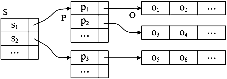
A sample of the SPO fact index.
As noted earlier, AMIE [21] and consequently AMIE+ [20], constituted a breakthrough in rule mining from RDF graph data. AMIE+ very well addresses the core of the rule mining problem – extracting an exhaustive set of rules, given RDF data and the right settings (typically user-set minimum support and confidence thresholds). At the same time, the algorithm as well as the accompanying implementation pay relatively little attention to the problems of data pre-processing, meta-parameter tuning, and post-processing; these steps are assumed to be addressed by external algorithms and software components.
Successful systems in the domain of rule mining from tabular and transactional data, such as the popular arules ecosystem [23], offer an integrated approach supporting the complete data mining life cycle: from pre-processing the input data to the selection of representative rules. Some other association rule learning packages also support automatic tuning of the rule learning meta-parameters, such as of the minimum support threshold [24].
An integrated approach is even more necessary in the linked data context as general algorithms for data pre-processing are difficult to apply to RDF datasets due to the different structure of inputs as well as outputs. For example, numerical attributes need to be discretized (quantized, binned, categorized [8]) prior to association rule mining. Discretization – as a pre-processing step – is supported in many libraries for tabular or CSV data, yet to our knowledge, there is no such tool for RDF triples.
Also, in the tabular or transactional context, it is typically computationally feasible to pre-process all available data. However, for RDF data such an non-discriminative approach to pre-processing may be prohibitively expensive. Instead, it is desirable to integrate data pre-processing (such as discretization) directly into the mining algorithm, so that only the values that can prospectively appear in the generated rules are processed.
Similar observations hold for the post-processing of results. In association rule mining from tabular or transactional data, it is sufficient for the mining algorithm to support only coarse requirements on the rules mined: it is computationally cheap to mine more rules and then apply finer requirements on the content of the mined rules within post-processing. However, the size of RDF KGs and the richer expressiveness of Horn rules make such an approach prohibitively expensive. While AMIE+ was very fast in processing synthetic benchmarks, as reported in [20], it may still be unusably slow or memory-intensive in practical tasks where – for example – the user does not know the precise minimum support threshold.
Some of the limitations described in this section do not only call for enhancing or extending the functionality of AMIE+ as a tool but also to inefficiencies we identified within the core AMIE+ algorithm. This is the case of repetitive and exhaustive calculations performed during the mining process.
Finally, some limitations relate to the lack of various features which were found useful for mining rules from transactional or tabular data. These include, such as the support for rule mining with the top-k approach or support for selection of most representative rules (by clustering or pruning). Other limitations stem from absence of features generally required from systems processing linked data, such as the support for multiple graphs.
Inability to process numerical data
Association rule learning algorithms do not work well with numerical data due to the downward closure property, which requires that not only the complete rule but also each subset of atoms composing it should meet the minimum support threshold. Since numeric attributes typically have many values, a single distinct value may not assure the required support. Such a value will thus be excluded from all generated rules.
Consider an RDF dataset with prices of public contracts. This dataset may include many facts containing a particular price of a contract. Each of these facts contains a numerical value at the object position related to a specific contract, e.g.,
An approach used to address this problem in association rule learning frameworks for transactional data, such as the arules library, is to replace multiple neighbouring distinct values of a numerical attribute with an interval of values.
Absence of the top-k approach
Decades of research in association rule learning and frequent itemset mining continuously show how difficult it is for users to set the minimum support threshold properly [7,57]. Similarly to the standard association rule learning, AMIE+ will generate all rules complying with the user-set support threshold. A too-small threshold leads to an enumeration of too many – millions and more – frequent itemsets (and consequently, rules), eventually resulting in an out-of-memory situation. In contrast, a too high threshold value may return no results.
Generating all rules already posed problems when association rule learning was executed on transactional databases like those collecting the contents of shopping baskets in a supermarket, where the analyst could still use their knowledge of the analyzed data to set these thresholds. This problem is further exacerbated when data may be very large.
In the top-k approach, the user is only returned the k rules with the highest values of the chosen measure, rather than all rules. This approach allows additional pruning strategies, alleviating or completely removing the risk of combinatorial explosion, the biggest problems of association rule mining [56,57].
Coarse rule patterns
Association rule learning tasks are in constant risk for combinatorial explosion, even on small datasets. This problem cannot be completely addressed by the top-k approach alone. Without additional guidance by the user, the top-k approach often generates rules that reflect patterns in data that are obvious or uninteresting for the user. For this reason, association rule learning frameworks provide various means for controlling the content of the generated rules. For example, in the arules library, the user can set a list of items (attribute-value pairs) that can appear in the antecedent and consequent of the generated rules. The LISp-Miner system15
AMIE+ adopts a similar approach to arules when it allows the user to provide a list of relations that should be included in (or excluded from) the body and head of the rule. In addition, there are several linked data specific settings relating to constants. The user can choose whether the constants are allowed, or even enforced, in all atoms of the generated rules. This approach, which is taken in AMIE+, does not take full advantage of the RDF data model. In particular, it is not possible to define independent, fine-grained constraints on subjects, predicates, and objects appearing in the discovered rules. For example, the user may wish to mine for rules that contain a triple with a specific value in the antecedent, such as:
During the refinement process, AMIE+ binds variables to constants in order to count the support for each fresh16
“Fresh” is a term used in [20] to denote a newly added atom.
This approach results in repetitive calculations, mainly in terms of variables binding. For example, the binding process starting from
AMIE+ first computes the value of support for each refined rule, and only afterwards it applies the pruning step based on a chosen support threshold. The same technique is used for the confidence calculation, where the algorithm first computes the confidence value and then filters the rules using confidence thresholds.
Searching of all triples instantiating the rule, which is necessary for computing the final value of confidence and support, may be very expensive. The process outlined above, used in AMIE+, can be made more efficient by terminating this counting early when it becomes clear that the final result of confidence or support will not meet the threshold.
Lack of support for multiple graphs
In Semantic Web terms, a KG identified by a specific IRI is called a named graph.17
AMIE+ does not support mining across multiple graphs such that one rule would contain resources from two or more different graphs. Also, AMIE+ is not able to resolve the owl:sameAs predicate to join resources from two different namespaces. For example, consider the following statements:
Association rule discovery can result in the generation of a high number of potentially interesting rules. Grouping – or clustering – of similar or overlapping rules can be effective for presenting the mining results in a concise manner to the end user.
Association rule learning frameworks, such as arules, provide, for this purpose, measures that express the similarity between association rules. Such support for rule clustering is not provided in the scope of AMIE+.
Another approach for addressing the problem of too many rules on the output is removal of some of the rules based on analysis of their overlap with respect to the input data. In rule learning literature, this supervised process is often called pruning [18]. While pruning may not be applicable for explorative association rule learning,18
E.g., the motto of the GUHA rule learning framework [25] is “GUHA offers everything interesting”, which translates as “all hypotheses of the given form true in the data”.
Some search strategies supported by ILP systems, such as ALEPH, are able to discover concise theories consisting of a small number of rules covering the input KG. Achieving the same coverage, AMIE+ mines all rules matching the user-specified mining thresholds without any pruning strategies, which would remove overlapping or redundant rules.
In the following, we present a collection of enhancements to AMIE+ that address the limitations summarized in the previous section.
Faster projection counting
AMIE+ recursively binds variables each time when new atoms are added. The binding process is important for finding valid connections to a rule being refined and for calculation of the support measure. However, it has a major impact on the overall mining time.
During the refinement process of a rule
The count projection query (described in Algorithm 2) binds all variables in the rule and enumerates all bound variants of the newly added atom connected to the rule with a cardinality. This process is inefficient in that it may redundantly bind variables in atoms that have already been mapped in the past (line 7 and 8).
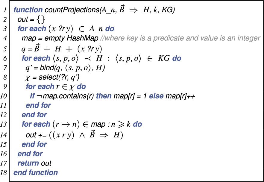
The AMIE+ count projection query
The bind function (line 7) maps all variables of atom H to constants of triple
In our approach, we try to reduce the number of calls to the binding functions (in line 6 to 12 of Algorithm 2). In the refinement process, the bindings of the head atom H should be performed only once. This process is described in Algorithm 3 within the refine function, which returns the set of atoms to be added into the rule being refined.

The RDFRules refinement process

The RDFRules bind projections query
The bindProjections function, described in Algorithm 4, is called for each instance of the head atom (lines 7 and 8). Notice that the binding is performed for all added closing and dangling atom variants together (lines 6 and 8). In each iteration, the bindProjections function returns a set of atoms
If the
The whole refinement process can be completed faster if we know that none of the found atoms in a certain moment can reach the minimum support threshold. The variable remainingSteps holds the number of iterations that still have to be done within the count projections query (lines 7 to 17). If
The bindProjections function invocation is composed of four phases. In the first phase, new atoms are divided into two sets: bound atoms
This approach eliminates a considerable number of repetitive calculations and makes AMIE+ much faster, especially for mining of rules with constants (see evaluation in Section 7).
As noted in Section 4.1, the standard solution used for handling numerical data in association rule mining is to perform the discretization (or binning) of numeric values with low frequencies into intervals. This step not only reduces the search space, but can also increase the support of some rules.
The proposed approach is performed within pre-processing, however, it is not completely decoupled from the mining phase. In order to avoid generation of intervals that are too narrow or unnecessarily broad for the purpose of the mining task, the user needs to provide the minimum head coverage threshold
Preliminaries
Data type determination As a first step, all predicates that have a numerical range have to be found. Most RDF serializations allow to directly encode data types, but it is up to the data producer to make use of this feature. Data types can also be determined from associated RDF vocabularies, which contain information about the range of the predicates.
Equal-frequency binning Equal-frequency binning is a common approach for discretizing numerical data for association rule learning, e.g., it is the default discretization method in the popular arules package. In the following, we discuss how this approach can be adapted for discretizing data in knowledge graphs.
In the context of our approach, the frequency of an interval I of predicate p is calculated as
Discretization in the rule head Let an instantiated atom
Discretization in the rule body The minimum support threshold depends on the minimum head coverage threshold and the head size of the rule; therefore, there are different minimum support thresholds for different heads. In AMIE+, the support is the number of correct predictions of the rule. Consider a rule with one atom A in the body. Such a rule predicts as many triples as is the size of this atom; therefore, if the following condition for the size of the atom A is not met, such a rule cannot reach or exceed the minimum support threshold:
Note that even if an atom does not meet the condition in Eq. (2), a rule containing this atom can still meet the minimum support threshold if this rule contains more than one atom in the body. For example, consider the following rule:
Proposed discretization heuristic
In the previous, we showed that – given the
Let P be a set of predicates occurring in the input KG that is constrained by the minimum head size threshold:
We define the upper bound of the minimum support threshold. This expresses the maximum possible atom size requirement for an atom A containing an interval I at the object position to be included in the rule with the highest head size.
Once
Tree of intervals Suppose we want to discretize the list
Data enrichment All created intervals generate new triples which are added into the input KG in the pre-processing phase before mining. For each triple

An example of the tree of intervals for some predicate where
The original data in the KG are preserved, since the newly added triples containing intervals use a different predicate (namely, one equipped with a tree-level suffix). Hence, this solution does not reduce the search space of the rule mining algorithm but rather expands it.
Discussion For any atom containing an interval with the size lower than
The lower and upper bounds reduce the number of constructed intervals and thus limit the overall increase in the size of the enrichment of the input KG generated by discretization. Nevertheless, the heuristic can incorrectly skip intervals with a low frequency, since, as previously discussed, if a body with more than one atom is considered, atoms with size lower than
Despite these limitations, the experiments (cf. Section 7.4) showed that the proposed merging of numerical values results in discovery of many new rules which contain predicates that would never appear in the output when mining directly from the original data.
Efficiently working with multiple graphs requires data structures supporting quads throughout the learning process. In AMIE+ this is not supported – the resulting rule always consists of atoms corresponding to triples.
In our approach, atoms in a rule may be extended with a fourth item that indicates the graph assignment; such an extended rule is called a graph-aware rule. This additional item is always generated as a specific graph resource and not as a variable. For instance,
The discovery of such a rule of course depends on the previously established identity of the resources across the used graphs. For instance, this condition is not met for concepts in YAGO and DBpedia, because the YAGO resource
Support for named graphs needs also to be reflected in the user-set pattern for rule learning. Before mining, the user can decide which atoms (or, how many of them) will be only based on triples from a certain graph, or whether to enable graph-aware mining at all. For example, the user can define the following pattern of a mining task where all rules have to consist of parts belonging to various graphs:
The inclusion of graph information in the rule mining process also requires an extension of fact indices, described in 3.6. These indices allow to check the affiliation to a given graph in constant time for all predicates (PG), predicate-subject pairs (PSG) and predicate-object pairs (POG), and for any predicate-subject-object triples (PSOG).
Improvements to expressiveness of rule patterns
AMIE+ only provides basic capabilities for restricting the content of the generated rules. These are generally limited to providing a list of predicates that can appear in the antecedent and consequent of the generated rules. Inspired by the LISp-Miner system, we defined a formal grammar-based pattern language (used in the RDFRules framework) for expressing more complex rule patterns in order to find desired rules for a specific task.
Consider
A rule pattern
(a rule pattern)
During the mining process, rules are pruned based on all input rule patterns. A rule pattern
Top-k approach
In the top-k mode, the result set contains at most k rules with the highest value of a chosen measure. This mining strategy alleviates the user from searching for the right mining threshold, and can also substantially reduce the mining time.
Our proposal is a variation on the top-k approach introduced by Wang et al. [56] for mining top-k frequent itemsets with the highest support from transactional data. The main mining phase includes searching for rules reaching a support threshold derived from a given head coverage threshold. If the support threshold or the head coverage is unknown we may set a k value as the maximum number of rules to be returned. For this case, the mining algorithm saves all found appropriate rules into a priority queue with fixed length k, where the head of this queue (the head rule) is the rule with the lowest head coverage. Once the capacity of the queue is reached the minimum support threshold is set to the head coverage of the head rule. Then the following rules are pruned based on this support threshold. At the moment when some new rule has its head coverage greater than the minimum, the head rule is removed from the queue, and the new rule is added. Then the minimum support threshold is modified by a next head element in the queue (see Fig. 4). The support threshold is continuously increasing during mining and the result set always contains at most k rules with the highest head coverage.

The top-k strategy using a priority queue with modification of the minimum support threshold.
The same strategy can be used for confidence calculation from a set of rules. Let k be the maximum length of the result rule set with highest confidences (standard or PCA). Once the capacity of the priority queue has been reached, the lowest confidence of the head rule is used as the minimum confidence threshold. This threshold is continuously increasing if the following rules have a higher confidence value.
Increasing the minimum confidence threshold minConf is important since it may speed up the confidence calculation. If the minConf value is set, then the following inequality must apply:
During the calculation of the body size, we can immediately stop the process as soon as the body size value is greater than the ratio between the rule support and minConf, because the rule is then guaranteed to have its confidence lower than minConf.
In order to cluster the rules, it is necessary to have some means of determining the similarity between an arbitrary pair of rules. The rule similarity can be computed from rule features, such as the content of the rule and the values of measures of significance.
Let the rules be represented with a matrix
It is straightforward to compare the measures of significance of two rules, e.g., the head coverage or the confidence values, as two numerical features. Nevertheless, in practice, for example within the arules library [23], rule clustering is mainly performed with respect to the rules content, in particular, using the similarity of atoms and their parts. Hence, for this purpose, we defined several similarity functions taking into account the content of the Horn rules.
Let an atom of a rule consist of a predicate p and of two atom items in the position of subject s and object o. These two atom items are either variables or constants. The similarity function between two atom items,
The similarity function for two predicates only tests their equality.
For the atoms
Suppose two rules U and V, where U has the length greater than or equal to the length of V,
While the generation of permutations (allowing to fit the two rules to one another) may look computationally demanding, for the rule lengths considered by RDFRules this overhead does not seriously impact the clustering performance, as witnessed by the experiments.
Rule pruning
For selection of the most representative rules from the list of mined rules we propose to adapt data coverage pruning, which is a technique that is commonly used in association rule classification [54].
This technique, described in Algorithm 5, processes input rules in the order specified in Listing 1. For each rule, the algorithm checks whether the rule correctly predicts at least one triple in the input KG (line 10). If it does, the rule is kept and the triple is discarded (for the purpose of pruning). If the rule does not classify any (remaining) triple correctly, it is discarded.

Rule data coverage pruning

Rule ranking criteria for rule pruning
In the list of rules mined by AMIE+, it is often the case that a single triple is correctly predicted by multiple rules. After data coverage pruning, many rules are removed, but it is still ensured that the reduced set of rules predicts the same set of triples as the original rule set (this is empirically evaluated in Section 7.7). Also, on transactional data, it has been empirically shown that the data coverage pruning (in combination with default rule pruning19
The well-known Classification Based on Associations (CBA) algorithm [40] essentially corresponds to data coverage pruning combined with ‘default rule pruning’. In default rule pruning, during the pruning process, we keep track of which rule led to the smallest number of misclassifications, when all rules ranked lower than this rule are replaced by a default rule assigning the most frequent class among the remaining instances.
While AMIE+ constitutes a breakthrough approach for rule learning from RDF data, the implementation accompanying the paper of Galárraga et al. [20] has several limitations in terms of practical usability compared to modern algorithmic frameworks for association rule learning from tabular datasets, such as the arules package for R [23], or Spark MLlib.20
In this section, we briefly describe a new framework for rule mining from RDF KGs called RDFRules, which is the reference implementation of the enhancements to AMIE+ described in the previous section, and is also used in our benchmarks (see Section 7).
RDFRules is freely available under the GPLv321
open-source license and is hosted on GitHub.22
Architecture of RDFRules.
The core of the reference RDFRules implementation is written in the Scala language. In addition to the Scala API, it also has a Java API, a RESTful service and a graphical user interface (GUI), which is available via a web browser. The Scala and Java APIs can be used as frameworks for extending another data mining system or application. The RESTful service is suitable for modular web-based applications and remote access. Finally, the GUI based on the RESTful service, can be used either as a standalone desktop application or as a web interface used to control the mining service deployed on a remote server. All modules are shown in Fig. 5.
Architecture
The architecture of the RDFRules core is composed of four main data structures: RDFGraph, RDFDataset, Index, and RuleSet. These structures are created in the listed order during the RDF data pre-processing and rule mining. Inspired by Apache Spark, each structure supports several operations which either transform the current structure or perform some action.
Transformations The data structures are formed in the following order:
A lazy transformation is not evaluated until a result of the transformation is required within an action.
Actions An action operation applies all pre-defined transformations on the current and previous structures and processes the (transformed) input data to create the desired output, such as rules, histograms, triples, statistics, etc. Compared to transformations, actions may load data into the memory and perform time-consuming operations. Actions are further divided into the streaming and batch ones. The streaming actions process data as small chunks (e.g., triples or rules) without large memory requirements, while the batch actions need to load all the data or a big part thereof into the memory.
Caching If several action operations are applied, e.g., with various input parameters, on the same data and with the same set of transformations, then all the defined transformations would normally be performed repeatedly for each action. This is caused by the lazy behavior of the data structures and the streaming process lacking the memory of previous steps. RDFRules eliminates those redundant and repeating calculations by caching the accomplished transformations. Each data structure has a cache method that can perform all the defined transformations immediately and store the result either into the memory or on the disk. The stored information can be reused when the already transformed data is to be further processed.
The RDFGraph structure is built once we load an RDF graph from either a file or a stream of triples or quads. For input data processing the RDFRules implementation uses modules from the Apache Jena24
framework, which supports a range of RDF formats including N-Triples, N-Quads, JSON-LD, TriG or TriX. Besides these standard formats, RDFRules also has its own native binary format for faster serialization and deserialization its data structures (like rules, triples, and indices) on/from a disk for later use. During data loading, the system creates either one or multiple RDFGraph instances. Multiple instances are created when the input data format supports and uses named graphs.An RDFGraph instance corresponds to a set of triples, on which applicable transformation operations are defined. These operations include filtering the triples using a condition, replacement of selected resources or literals, and merging numeric values using discretization algorithms. The transformed data may be exported to an RDF file. Several further operations focus on data exploration. These include the statements aggregation on histograms of triple items, the predicate ranges determination, and the triples counting.
The RDFDataset structure is created from one or more RDFGraph instances. It is composed of quads where the triples are additionally associated with a particular named graph. This data structure supports transformation of all triples/quads within a dataset, as well as in the case of a single graph, with or without regard to the graphs assignment.
Before the mining, the input dataset has to be indexed in the memory, which allows for the fast enumeration of atoms and computation of the measures of significance.
In the first phase of the indexing, each element of the triples, whether an identifier or a literal, is mapped into a unique number. This mapping is stored in a special hash map and eliminates any duplicates.
In the second phase of the indexing, the program only deals with the mapped numbers and creates the six fact indices described in Section 3.6. These indices are in one of the two modes: preserved or in-use. The preserved mode keeps the data in the memory for the whole duration of the index object, whereas the in-use mode only loads the data into the memory if the index is needed and after the use of the index, the memory is again released.
The Index instance can be created from the RDFDataset structure or loaded from the cache. The image of the fact indices can, therefore, be saved on the disk for further reuse. The Index structure contains the prepared data and has operations for rule mining using the AMIE+ algorithm.
Rule mining
RDFRules implements the extensions to the AMIE+ rule mining algorithm covered in Section 5. Besides the indexed data itself, the values of three kinds of parameters also enter the mining phase in RDFRules; these parameters are (pruning) thresholds, rule patterns, and constraints.
Pruning thresholds In addition to the thresholds defined in AMIE+, RDFRules also offers the top-k approach (see Section 5.5), and the timeout threshold, which determines the maximum mining time. All the mining thresholds are listed in Table 1. Notice that the list of thresholds does not contain any confidence measures. These additional measures of significance can only be calculated after the main mining phase within the RuleSet structure.
Available user-defined pruning thresholds used in the mining process in RDFRules
Available user-defined pruning thresholds used in the mining process in RDFRules
Rule patterns All the mined rules must match at least one pattern defined in the list of rule patterns. If the user has an idea of what kinds of atoms the mined rules should contain, this information can be defined through one or several rule patterns. The grammar of the rule pattern is described in Section 5.4. Since the process of matching the rules with patterns is performed during the mining phase, the enumeration of rules can be significantly sped-up.
We can define two types of rule pattern: exact and partial. The number of atoms in any mined rule must be the same as in the exact rule pattern. For a partial pattern, if some rule matches the pattern, all its refined extensions also match the pattern.
Constraints Finally, the last mining parameter specifies additional constraints, thus further shaping the output of the mining. Here is a list of the implemented constraints that can be used:
OnlyPredicates(x): the rules may only contain the predicates from the set x.
WithoutPredicates(x): the rules must not contain any of the predicates from the set x.
OnlyVariablesAt: restricts to rules where constants are disabled at an atom position or all atom positions.
WithoutDuplicatePredicates: disallows rules containing the same predicate in more than one atom.
GraphAwareRules: the atoms in the discovered rules will be extended with information on their graph of origin.
Mining The mining process can be run in different behavior modes, with respect to the entry thresholds and constraints. Compared to the pure AMIE+ implementation, RDFRules does not calculate the confidence while browsing the search space of possible rules, thus saving time. Additionally, it applies various extensions described in Section 5. The rule mining process is performed in parallel (see Algorithm 1) and tries to use all available cores.
The mining result is an instance of the RuleSet structure which contains all the mined rules conforming to the input restrictions.
The RuleSet is the last defined data structure in the RDFRules workflow. It implements the operations for rule analysis, calculation of additional measures of significance, rule filtering and sorting, rule clustering and pruning, and finally, an export of the discovered rules for use in other systems. Every rule in the rule set consists of the head, the body, and the values of the measures of significance. The basic measures of significance are: rule length, support, head size and head coverage. Other measures may be calculated individually on user demand within the RuleSet structure. These measures include: body size, confidence, PCA body size and PCA confidence. The rules can be filtered and sorted according to all these measures.
RDFRules supports rule clustering with the DBScan algorithm [15], using similarity functions proposed in Section 5.6. The clustering process returns an assignment to a cluster for each rule based on input parameters including selected features, a minimum number of neighbors to create a cluster, and a minimum similarity value for two rules to be in the same cluster. The user can also opt to use similarity counting to determine the top-k most similar or dissimilar rules to a selected rule.
All the mined rules are stored in the memory, but, as in the case of the previous data structures, all transformations defined in the RuleSet are lazy. Therefore, this structure also allows to cache the rules and transformations on the disk or the memory for repeated usage. The complete rule set (or its subsets) can be exported and saved into a file in a human-readable text format or in a machine-readable JSON format.
Comparison to AMIE+ implementation
In the following, we will briefly compare the features of the AMIE+ implementation by AMIE+ authors25
Feature comparison between the reference AMIE+ implementation and RDFRules
We performed two kinds of experiments. Within the first group of experiments, we compare our proposed enhancements presented in Section 5 and implemented within our RDFRules framework with the original implementation of the AMIE+ algorithm. The second group of experiments is focused on evaluation of the newly proposed enhancements and algorithms. In particular, we evaluate discretization of numerical attributes proposed in Section 5.2, mining across multiple graphs (Section 5.3), rule patterns (Section 5.4), top-k approach (Section 5.5), clustering (Section 5.6), and rules pruning (Section 5.7).
Experimental setup
For our experiments, we mainly used the YAGO2 core dataset and YAGO3 core samples of yagoLiteralFacts, yagoFacts and yagoDBpediaInstances available from the Max Planck Institute website.26
For more time consuming tasks we used DBpedia 3.8 with person data and mapping-based properties. For other experiments we used samples of mapping-based literals and mapping-based objects. The number of triples and their unique elements for each dataset are shown in Table 3.All the mining tasks are set with the minimum head size threshold 100 and maximum rule length 3. Unless explicitly mentioned, the number of used threads is set to 8. Each experiment is composed of various mining thresholds, constraints, patterns, the input dataset, and a selected framework (AMIE+ or RDFRules). Each experiment was executed 10 times. The experimental outcome consists of the average mining time together with the standard deviation and the number of found rules.
All experiments were launched on the scientific grid infrastructure of the CESNET MetaCentrum.27
This grid architecture offers up to several hundred CPUs to be used per machine. For our purpose we used from 1 to 24 cores per experiment on a machine with these parameters:CPU: 4x 14-core Intel Xeon E7-4830 v4 (2 GHz),
RAM: 512 GB,
OS: Debian 9.
A part of the implemented RDFRules framework is the Experiments module,28
within which all the experiments described below were conducted. Hence, all the reported experiments can be easily reproduced.Used datasets in experiments
In this section we compare our proposed and implemented enhancements of the AMIE+ algorithm with the original AMIE+ implementation.29
The mining runtime of AMIE+ and RDFRules with various settings
We performed two experiment types: 1) mining rules only with variables at the subject and object positions – and 2) mining rules with enabled constants. The mining process involves the computation of both types of confidence, i.e. standard confidence and PCA confidence. The results are reported for fixed standard and PCA confidence threshold 0.1 (MinConf+PCA) and a various minimum head coverage threshold (MinHC). RDFRules does not use the perfect rules pruning30
As an optional feature, AMIE+ stops refining rules as soon as confidence of the rule reaches 1.0.
The number of output rules for RDFRules may be different from AMIE+. This is because AMIE+ does not return to the output the rules whose all parents have a higher confidence measure. A parent of the rule is a rule derived from the given rule by removing any one atom from its body. RDFRules has this functionality turned off by default; therefore, it can return more rules. This filtering is performed when the output rules are returned, and thus it does not affect the reported mining runtime.
The comparative experiments were launched for the YAGO2 core dataset and the DBpedia 3.8 dataset. Some selected tasks, their settings, and results are shown in Table 4. The Diff column contains the difference between the runtimes of AMIE+ and RDFRules. The Rules column contains the number of rules returned by AMIE+ and RDFRules.
Beside the Table 4 the results for the YAGO2 core dataset are also shown in Fig. 7 for mining without constants, and in Fig. 6 for mining with constants. We observed that for more difficult tasks with lower head coverage thresholds, which generate a larger set of rules, RDFRules is faster than the original AMIE+. On the contrary, for simpler tasks lasting several seconds and without constants, both approaches are almost at the same level of mining time.

AMIE+ vs RDFRules: runtime comparison for rule mining with constants for YAGO2 core.
Our performance improvements proposed in Section 5.1 have a considerable impact on mining with constants. For instance, the mining task with constants with
The experiments also revealed that the original AMIE+ implementation assigns the individual jobs less efficiently into multiple threads when mining with constants. In our experiments, RDFRules used 99% of the CPU cores, whereas AMIE+ used only around 40%. To have a baseline, we also tried to mine rules with constants in a single thread. In this setting, RDFRules was still almost twice faster than AMIE+ (see the last row in Table 4). The degree to which the two systems scale when mining with constants is depicted in Fig. 8.

AMIE+ vs RDFRules: runtime comparison for rule mining without constants for YAGO2 core.

Scalability of RDFRules and AMIE+. Mining with constants and with
For the DBpedia 3.8 dataset, we used default settings with minimum head coverage 0.01. The maximum mining time was set to two days. Each experiment was launched only twice with regard to more time consuming processes.
For AMIE+, the task of mining rules only with variables was not completed within two days. Hence, we tried to enable the confidence approximation where the task took around 7 hours, whereas RDFRules computed it without any approximation technique in 15 minutes.
The task of rule mining with constants was not finished within two days for both AMIE+ and RDFRules. The problem is the combinatorial explosion since the number of possible rules with constants is enormous for this task and dataset. Hence, we simplified the task for RDFRules to instantiate only variables at the lower-cardinality side of the predicate (this setting is not available within AMIE+). This task was successfully completed within 27 minutes and more than 380k rules were found (see Table 4). After increasing the minimum head coverage threshold to 0.15 the mining task was completed in 18.5 hours for RDFRules where more than 1.5M rules were found. For AMIE+ (also with the approximation technique) the task was not finished in 2 days.
Evaluation of the top-k approach and rule patterns
This section reports on results of experiments of enhancements specific to RDFRules: the top-k approach, confidence calculation, and rule patterns. For the top-k approach, described in Section 5.5, we launched the same tasks as in the previous set of experiments with the difference that the result set contained just the top 100 rules with the highest head coverage. We also tried to compare confidence computation with vs. without the top-k approach. Finally, we compare the mining time with search space constrained with rule patterns with the time required to mine all rules followed by subsequent filtering by a particular pattern.

RDFRules rule mining, only with variables (logrules) and instantiated (const), with vs. without the top-k approach.
The mining runtime of the RDFRules top-k approach
Figure 9 and Table 5 show how the top-k approach improves the performance of mining if only a subset of all rules with the highest head coverage is desired by the user.
As described in Section 5.5, the top-k approach can also be used to speed-up confidence computation (standard or PCA). Table 6 contains results for confidence computation (both standard and PCA) of 100,000 rules. This is compared with searching for the top 100 rules with the highest confidence.
Runtimes of the confidence computation for 100,000 rules compared with the top-k approach. Settings are:
Another experiment was conducted to benchmark the mining with partial patterns, which were introduced in Section 5.4. We launched two tasks for two rule patterns. The first one emulates the situation when the user-specified the head of the rules to be discovered:
Mining with and without rule patterns

An example of rules mined by RDFRules with patterns
We used the proposed discretization technique (described in Section 5.2.2) based on trees of intervals for the DBpedia literals sample dataset. The minimum head size threshold and the minimum head coverage threshold, required for the calculation of
The pre-processed input KG was then used in the mining process. First, we observed the number of mined rules for both variants of mining from the input KG: with vs. without the pre-processing.
Next, we evaluated the discretization on the task of knowledge graph completion, where we again compared the results generated with and without the discretization. The output rules were filtered by the minimum PCA confidence threshold set to 0.8. Consequently, all filtered rules were used to predict triples (explained in Section 3.3).
From the predicted triples T, we only took such triples
The filtering of the output triples by the above formula assures that the Partial Completeness Assumption is preserved not only at the level of the rule (which has to satisfy the PCA confidence criterion as whole) but also at the level of the individual triples supplied to the KG.
Data size of the DBpedia literals sample dataset before and after the discretization process using trees of intervals
Output comparison of results after mining with or without the discretization phase
Table 8 summarizes the results from the various discretization processes. The header contains the number of all triples, all predicates, and all predicates that had a numerical range before the discretization process. The following rows show how many new triples and predicates were created after the discretization using the minimum head coverage threshold.
Table 9 shows that after the discretization, the system discovered many more rules (ca. 300 times more) and predicted many more new triples, even for higher thresholds, where originally no rules were found. For example, we predicted the following new triple, which is missing in the original KG:
It should be noted that the discretization does not only have benefits, but also extends the mining time due to the expansion of the hypothesis space. In the performed experiment, the mining time was up to six times longer.
RDFRules is able to merge multiple RDF KGs together, resolving their integration by the owl:sameAs predicate, which is described in Section 5.3. This linking is taken into account in the mining phase; therefore, discovered rules can contain atoms from different graphs.
We launched the rule mining process with minimum head coverage threshold 0.01 and enabled constants at the object position, separately for the YAGO3 sample and for the unified DBpedia sample (literals + objects). Subsequently, we merged the YAGO and DBpedia graphs using the yagoDBpediaInstances subset, containing the owl:sameAs linking, which is also part of the YAGO3 sample. Finally, we launched the rule mining process for the whole dataset consisting of these two different KGs.
The number of output rules from all tasks (YAGO, DBpedia, YAGO+DBpedia) is written in Table 10. For the merged YAGO+DBpedia dataset, a large number of new rules (998,240) containing atoms from both KGs were discovered. The mining time for YAGO+DBpedia is slightly longer (ca. 1.5x) than the sum of the mining times for each KG separately.
Evaluation of clustering
The goal of clustering is generally to find cluster assignment minimizing the inter-cluster similarities and maximizing the intra-cluster similarities. For our experiment, the clustering was based on the rule content similarity function described in Section 5.6. The evaluation was focused on the quality of cluster assignments.
First, we needed a set of rules as an input for the clustering process. We used the YAGO2 core KG for mining the top 10,000 rules with constants (minimum head coverage threshold 0.01). Then, for the output rules, we launched clustering with the DBScan algorithm [15] with the minimum number of neighbours (region density MinPts) fixed to 1 for all experiments. The second element of the setting was the minimum similarity threshold used as the inverse distance radius ϵ parameter of DBScan. For ϵ, we varied the threshold value.
Once the rules had been assigned to the clusters, it was possible to evaluate the quality of the assignment based on the overlap of clusters (inter-cluster similarity), and the similarities among rules inside a cluster (intra-cluster similarity). Let
The proposed QI is inspired by the average Silhouette Index [52]. The difference is that we take into account rule similarities instead of distances and the intra and inter cluster similarities are computed with the more straightforward way without having to calculate similarities among all rules across all clusters, which is very time consuming. The range of values of the QI is from
In the rest of this section we will denote the subset of the input KG containing exactly those (distinct) triples that instantiate any atom from the body or from the head of a rule as the matching subgraph of this rule.
Rules and runtimes comparison after mining for merged and separated KGs
Rules and runtimes comparison after mining for merged and separated KGs
Intra-cluster similarity Let
The weight is important since more general rules can match many more triples than more specific rules. For example, the following rule
Inter-cluster similarity Let
Results For each clustering task, beside the QI, we calculated the average intra-cluster and inter-cluster similarity. All these measures, along with clustering runtimes and the number of created clusters, are shown in Table 11.
Results of clustering for 10,000 rules by the DBScan algorithm (
The table shows that the average intra-cluster similarity is much greater than the average inter-cluster similarity, which is desired. In our experiments, the highest value of the QI was obtained for MinSim
In this section, we demonstrate the effectiveness of the pruning technique described in Section 5.7 on the YAGO2 core dataset. First, we mined top-k rules with different values of k and with the minimum standard confidence threshold set to 0.1. After that, we sorted rules by the confidence measure in descending order and applied the pruning step.
All results are summarized in Table 12. We compared the number of output rules with the number of rules after pruning. Notice that the number of rules after pruning increases logarithmically compared to the sizes of the set of rules before pruning. The table also shows that the number of all correctly predicted triples from the input KG by rules before and after pruning is still the same.
The number of rules and correctly predicted triples, before and after pruning for YAGO2 core. The Runtime column shows the time spent by pruning
The number of rules and correctly predicted triples, before and after pruning for YAGO2 core. The Runtime column shows the time spent by pruning
In this paper we have presented a set of extensions and enhancements to AMIE+, a state-of-the-art approach for mining Horn rules from RDF knowledge graphs. The primary aim of our work was to contribute to resolving the main challenge related to association rule learning (not only) from knowledge graphs – making it easy for the user to extract meaningful rules, without having to repeatedly change the mining parameters due to either a lack of results or a combinatorial explosion thereof. By giving the user the option to automatically group similar rules or to remove redundant rules, the result of rule learning remains explainable even when tens of thousands of rules are discovered. Other presented extensions allow for mining rules spanning multiple graphs, support for numerical data, and substantial performance enhancements in some special cases, such as when mining with constants or when mining with many CPU cores.
In a number of experiments, we have shown performance improvements of the individual extensions. More than an order of magnitude improvement compared to AMIE+ has been observed when mining for rare patterns, e.g., anomalies, which requires a very low head coverage threshold.
A reference implementation of the proposed approach is available as open source hosted on GitHub.33
A promising direction for extending RDFRules is that of adding support for RDF schemas and ontologies, which would involve resource types with hierarchies into the mining process. Another challenging problem is that of matching the capabilities of the new generation of ILP systems, which, for example, support predicate invention and recursion [10]. We should also carry out comparative experiments with AMIE 3 as the very recently announced AMIE+ successor (thus being a ‘close sibling’ of RDFRules). Although the system currently supports multi-threading on a single machine, we would also like to add support for distributed mining and memory scaling on multiple nodes. Finally, RDFRules produces logical rules with a possibly complex structure, which may be found difficult to understand by some users. Thus, research into the human-perceived interpretability of logical rules is urgently needed. From the usability perspective, a valuable addition could be the addition of automatic tuning of mining thresholds, possibly by adapting one of the algorithms proposed for tabular data in [34]. In terms of applications, we consider investigating to what extent RDFRules can complement the recent generation of ILP systems such as Metagol [11] or MIGO [28] in the domain of learning game strategies. Specifically, we consider using RDFRules for learning an initial set of rules, leveraging the speed of its base association rule learning approach, and then refining these rules in the established ILP frameworks.
Footnotes
Acknowledgements
We are grateful to our three reviewers for detailed feedback, which resulted in many improvements of the article. Computational resources were partly supplied by the project “‘e-Infrastruktura CZ” (e-INFRA LM2018140) provided within the program Projects of Large Research, Development and Innovations Infrastructures. TK was supported by the Prague University of Economics and Business, Faculty of Informatics and Statistics, via the long-term institutional support of research activities, and by the IGA 43/2020 project. VZ and VS were partially supported by the CSF project no. 18-23964S.