Typology-based semantic labeling of numeric tabular data

Abstract

A lot of tabular data are being published on the Web. Semantic labeling of such data may help in their understanding and exploitation. However, many challenges need to be addressed to do this automatically. With numbers, it can be even harder due to the possible difference in measurement accuracy, rounding errors, and even the frequency of their appearance. Multiple approaches have been proposed in the literature to tackle the problem of semantic labeling of numeric values in existing tabular datasets. However, they also suffer from several shortcomings: closely coupled with entity-linking, rely on table context, need to profile the knowledge graph, and require manual training of the model. Above all, however, they all treat different types of numeric values evenly. In this paper, we tackle these problems and validate our hypothesis: whether taking into account the typology of numeric data in semantic labeling yields better results.

1. Introduction

The number of structured data published on the web is constantly growing thanks to initiatives such as the Open Data movement (e.g., data.gov1

¹

https://www.data.gov/

) and more specialized platforms (e.g., Kaggle,2

²

https://www.kaggle.com/

Figshare,3

³

https://figshare.com/

data.world4

⁴

https://data.world/

). One of the most fundamental problems is enabling the understanding of the dataset content, which could be beneficial for different groups, such as researchers working on the expansion of Knowledge Bases5

⁵

In this work, we use the terms “Knowledge Base” and “Knowledge Graph” interchangeably.

(KB) [27], for data scientists who found a dataset and want to use it for their knowledge discovery task [10], or for expanding meta-data describing a dataset which could be utilized further for data search (e.g., Google Dataset Search Engine [19]).

There are several approaches focusing on the problem of understanding the semantic meaning of the content of datasets [1,6,9,17,24]. They focus on detecting semantic labels for specific dataset cells (such as [6]) or assigning semantic labels to the whole column (such as [17,24]). However, the majority of the existing efforts focused mainly on textual columns with not much attention being drawn to numerical columns present in the dataset. Recently, the research focusing on the problem of assigning semantic labels to numerical columns in a dataset started to get traction. In the work of Mitlöhnert et al. [15], it was pointed out that numerical columns are the most popular column type among datasets from several open data portals.

The approaches targeting the annotation of numerical columns need to tackle different issues than the ones developed for textual columns. It can be harder due to the possible difference in measurement accuracy, rounding errors, the frequency of their appearance, or different values being reported by different resources (e.g., population data). Multiple approaches tried to solve this problem, but they also suffer from several shortcomings: closely coupled with entity-linking (each number in the numeric columns has to match a numeric property of an entity in the knowledge graph), rely on table context (e.g., the URL of the page, the caption of the table, the surrounding text), need to profile the knowledge graph (e.g., create a model of the whole knowledge graph, build inverted index), and require of manual training of the model. Above all, they treat different types of numeric data evenly.

In this work, we expand our recent work [1], where the semantic labeling of numerical values is performed using fuzzy clustering. Our previous work shows that it is possible to semantically annotate numerical columns in tabular datasets without applying object matching or entity linking techniques. However, since all numeric data were treated uniformly, there were cases where the approach mislabeled some of the numeric columns. Hence, in this work, we expand the approach to take into account the typology of the numeric data. We hypothesize that taking into account the typology of the numeric data in the semantic labeling process results in better accuracy. We propose a typology of numbers based on the typology proposed by others [5,16,28] for the process of semantic labeling. We take different approaches to annotate each of them.

The contributions of this paper can be summarized in the following points:

• We introduce an extension of the typology of numerical values presented in the literature. This extension includes the concept of sub-type, where a type can be divided further into sub-types.

• We propose a way to detect the type of a list of numerical values based solely on its content, without external resources or context.

• We propose a new approach to label numerical columns in tabular data taking into account the type of numerical values in a column.

The rest of the paper is organized as follows. We begin by reviewing the typology of numbers in Section 2. We review the state-of-the-art in Section 3, and we explain the problem statement in Section 4. We introduce the typology of numerical values in Section 5 and show how we can detect each of the (sub-)types in Section 6. In Section 7, we show how we extract data from a knowledge graph and construct the model which we use for the semantic labeling in Section 8. We evaluate our approach in Section 9 and conclude the paper in Section 10.

2. Background: Types of numbers

Mosteller and Tukey said: “Just writing in digits does not make a number” [16]. On the other hand, Stevens [28] refers to nominals as numbers,6

⁶

More discussion on the definition of numbers is mentioned by Russell [26].

but he (along with Mosteller and Tukey [16]) agrees that numbers can carry different meanings, and hence the different types. Stevens [28] proposed four types of numbers: nominal, ordinal, interval, and ratio.

Nominal where digits are just like names, so they do not imply extra meanings such as order. For example, if we have two names, John and Adam, we cannot say that the name John is greater (or less) than the name Adam. An example of nominals are the digits printed on the shirts of football players: they only distinguish the players, but it does not have a “greater than” or “smaller than” concept to it. So, the only operation available is to compare two nominals, whether they are the same or not.

Ordinal type implies an order among a set of elements. So one appears before the other. There is the concept of greater than (or less than) between two elements. An example would be ordering the dishes in a menu from the most favorable to the least favorable, or differences in responses in satisfaction surveys between “very satisfied” and “somewhat satisfied” [11]. However, there is no regard to the difference between the two items. For example, if a person likes dark chocolate more than white chocolate ( $\mathit{dark}\mathit{chocolate}\mathrm{>}\mathit{white}\mathit{chocolate}$ ), there is nothing about the difference between their likeness of dark chocolate and white chocolate. Such an operation could be referred to as “illegal” [28].

Interval scale is used to denote the increase or expansion in some way on a scale. A classical example presented by [28] is the use of two different scales to measure the temperature. Humans use Centigrade and Fahrenheit, and we have a way to transform the temperature from one scale to the other. The intervals are the same (e.g., the difference between 10 and 20 degrees Celsius is the same as the difference between 25 and 35 degrees Celsius) [11].

Ratio scales refer to things we measure that contain a real zero such as counts, fundamental, and derived ratios. Counts represent the number of elements or occurrences (e.g., number of eggs in a basket). Fundamental ratio represents measurements taken directly (e.g., when the width of the table is taken directly using a measuring tape or a ruler). Derived ratio is the mathematical function of the magnitudes of a simple (fundamental) ratio measure (e.g., computing the speed of a car using a measured time and distance). The difference between ratio and interval is the existence of a true zero.7

⁷

Also referred to as “real” and “absolute”.

For example, when we talk about the temperature, there can be an agreement on a zero value (for example 0 in Celsius and 32 in Fahrenheit for the freezing point of water at 1 atmosphere unit), but it is not a true zero point (it does not mean a complete absence of temperature). Such a point is referred to as the “starting” point [11,16].

Some measures are not considered by Stevens, such as the cyclical measures [5]. An example of such cyclical measures is the angle; Chrisman said: “the direction 359° is as far from 0° as 1° is” [5]. The added levels presented by Chrisman are: Log-interval, extensive ratio, cyclic ratio, derived ratio, counts, and absolute.8

⁸

Chrisman suggestion is to consider them as separate types.

Log-interval is similar to the interval scale with the scaling happening on the exponent level. Extensive ratio is the same as the fundamental ratio explained by Stevens (e.g., the width of a book). Cyclic ratio is the same as the extensive ratio where it is bounded and repeat. Absolute is when a scale is predetermined and cannot be transformed while preserving the meaning.

Mosteller and Tukey have a similar categorization: names (nominal), grades and ranks9

⁹

Ranks are numbered while grades are labels (e.g., A, B,…).

(ordinal), amounts (fundamental ratio), balances10

¹⁰

It is similar to log-interval but also is a ratio, so we consider it here a derived ratio.

(derived ratio), counts, counted fractions11

¹¹

It is not exactly equal as absolute; it is more general than counted fractions, but it is enough approximation for our purpose in this paper.

(absolute). However, it lacks the following: interval,12

¹²

Even though Mosteller and Tukey warns the reader when re-expressing zeros, they do not create a separate category for it.

log-interval, and cyclical ratio.

Types of numbers are also referred to as kinds of numbers, scales of measurement, and levels of measurement [5,11,16,28]. We present a summary of the types in Table 1.

Table 1

Typology summary

Type	Description
Nominal	Numbers as names without any order among the set of elements (e.g., social security numbers)
Ordinal	Imply order among the set of elements (e.g., winners of a race)
Interval	Measurements without a real zero (e.g., temperature of a cup of tea in Celsius)
Ratio	Measurements with a real zero (e.g., length of a table in meters)
Log Interval	Similar to interval but on the exponent-level
Counts	Number of elements or occurrences (e.g., number of eggs in a basket)
Fundamental Ratio	Measurements taken directly (e.g., width of a book)
Derived Ratio	a mathematical function of the magnitudes of the fundamental ratio
Cyclic Ratio	Fundamental ratio that is bounded and repeats (e.g., angles)

3. State-of-the-art

The topic of semantic annotation for tabular data has been of interest to search engine companies as well as for the semantic web community for the last two decades. Different techniques have been used to perform this task: graphical probabilistic models [8,12,30,33], linear regression [4,21], decision trees [29], hierarchical clustering [17], and support vector machine (SVM) [12], among others.

These techniques need to be applied to computed information extracted from the data, which are referred to as “features” in machine learning. Cafarella et al. [4] use attribute correlation statistics computed from the crawled web documents and schema coherency score. Features like the number of hits on the tables [4], column types [8,12], text similarity [12,21], and the relation between columns/entities [8,12,30,32] are all used and shown to be the main drivers of high-quality annotation. Nishida et al. [18] use a long short-term memory (LSTM) network in order to obtain a semantic representation of each cell in the table. Statistical tests to compare distributions from different samples have also been adopted, especially for dealing with numerical data [9,17,21,22].

Fig. 1.

Outline of inputs and outputs of the problem tackled in this work. Light gray highlights the inputs to the semantic labeling approach.

From our review of the state-of-the-art, we can see that there are two kinds of learning sources (training sets). The first kind uses knowledge graphs such as YAGO [12] and DBpedia [17,24] to create learning sets. Others are more focused on learning from scraped web pages, which do not provide such ease to focus on a specific domain [4,8,29,32]. Despite the fact that these approaches may be automatic or semi-automatic,13

¹³

We are not referring here to the gold standards that are built manually or the semantic models that are constructed by domain experts.

some of them require manual actions (e.g., provide predefined conversion rules [24,33], a blacklist of properties [17] to improve the accuracy and abbreviations resolution [24,33] while others, such as [14], rely on experts to annotate columns to semantic properties. Approaches, such as [9,20,34], base their analysis of numerical columns on the context of the subject column – which is the column that acts as the primary key of the table [34]. We also found that they treat all numerical columns and their values in the same way, not taking into account the type of numerical values except for [20]. Oulabi et al. [20] divide numeric values into Quantity and Nominals. This is not really a typology; it is to distinguish whether to treat the values as measurements (Quantity) or as text (Nominals). Their detection algorithm of the type of numerical data (Nominal or Quantity) relies on the data in the knowledge graph.

Fig. 2.

An example of types and sub-types.

In this work, we propose a typology of numerical values. We detect the type of numerical values and then use it to improve the performance of semantic labeling without matching the exact numbers to a property of a matched entity, relying on an ontology, profiling knowledge graphs, manual elimination of properties, or tweaking of parameters (that are knowledge graph dependent).

4. Problem statement

We define a dataset as a collection of tables, and each table is composed of multiple columns. Columns in a table may consist of numerical values, textual values, or a combination of both. In this work, we focus on numerical columns and exclude any textual context, such as the header of the column or any text within column cells. This results in each numerical column being represented as a collection of numerical values. The problem statement of this work could be summarized as follows:

Given a collection of numerical values of a specific type, a class describing the content of a table and a target knowledge base, return a list of properties in the knowledge base that most likely correspond to those numerical values, ordered by likelihood scores.

Figure 1 outlines the inputs and outputs of the semantic labeling approach.

5. Typology of numerical columns

In this work, we adopt the typology presented by Stevens et al. [28] as a base, and we build on top of it. This is because it is more suitable for the detection of different types, as we explain in Section 6. We extend two of the high-level types (nominal and ratio) into sub-types. We based our work on types discussed by Tukey [31], Mosteller et al. [16], and Stevens et al. [28].

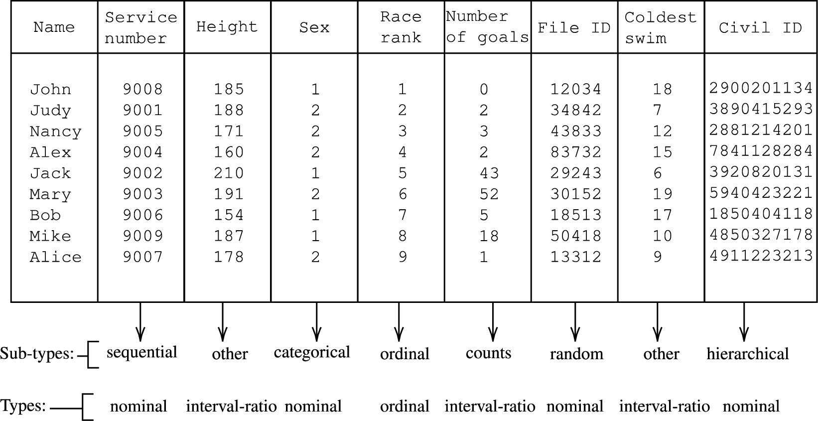
Example We present a table with numerical columns, and we assign to each column a type and a sub-type (Fig. 2). The table is about military individuals. The first column contains the first names, so it is not a numeric column. The second column represents the “service name”. Each person has a unique service name showing on their uniform. The 3rd column represents the heights in centimeters. The column after that is about the “sex” of the people, so males are denoted as 1 and 2 for females. The “Race rank” column represents the order of the winners of a race held for those people (e.g., 1 means the person came first, 2 means the person came second place). The sixth column represents the number of goals each of the players scored in a season. The 7th column contains the internal identifiers of the personal files (there is a file containing personal information about each individual). The following column contains the coldest temperature (in Celsius) of the water in which the corresponding person was able to swim. The last column represents the civil id for each person. We discuss further the construction of the civil ids later in this section.

5.1. Nominal

Nominals are labels that are composed of digits. They are used to distinguish between things represented by different labels. Such are used instead of names because it is easy to check for uniqueness compared to names as multiple people can share the same name.14

¹⁴

As the case of baseball https://en.wikipedia.org/wiki/Uniform_number_(Major_League_Baseball).

It could be impossible to know whether given numerals in a column are nominal or not without having extra context. However, understanding how these numerals are generated can give us some insights. To ensure the uniqueness, some use a sequence of natural numbers (e.g., military units). Some start from large numbers, and the sequence would be, for example, organized as (90000, 90001, 90002,…). We refer to such sets of numbers as sequential. In Fig. 2, an example of sequential sub-type is presented in the column “Service number”, where the values range from 9001 to 9009.

In other cases, the number is a combination of segments, where each segment has a meaning [13]. A segment of a number can mean the unit of the soldier (in the case of military personnel),15

¹⁵

https://en.wikipedia.org/wiki/Service_number

or the date of birth [13], sex, place of birth, and usually the last part of such nominal number ends with a random number or sequence [13]. Such numbers are referred to as hierarchical (see Fig. 3).

The third sub-type of nominal is the general case where a number represents a group, sometimes referred to as categorical. An example of such data can be seen in the column “sex” in Fig. 2, where 1 is used to represent males and 2 to represent females.

The fourth kind of nominal is something that is either randomly generated (like automatically generated ids in software), or they only make sense for the platform like addresses in memory (column “File ID” in Fig. 2).

To summarize, we identify four sub-types of nominals: 1) sequential; 2) hierarchical; 3) categorical; and 4) random.

Fig. 3.

An example of hierarchical sub-type.

5.2. Ordinal

It is the same ordinal scale we explained in Section 2. It represents a rank with no regard to the difference. For example, it is concerned with the order of the winners (1st, 2nd,…), but with no regard to how many seconds it took each of the runners to complete the race. It also has no concern about how much faster the first runner was from the 2nd (in terms of the speed difference).

5.3. Interval and ratio

We introduce two sub-types: counts and other. Following [28], we define the sub-type counts (also known as cardinal numbers) as the number of instances or occurrences of something. An example of this is the number of goals scored, as shown in Fig. 2.

In fundamental ratio, the numbers tend to have fewer digits in the fraction parts than derived ratios because they are measured, and the accuracy is bound by measurement tools while the derived ratio is a function that could produce more fractions (more digits after the decimal point). For example, if we have a circle with a radius of 0.13 (which is a fundamental ratio), and we want to calculate the area of this circle16

¹⁶

$\mathit{area}=0.5\ast 2\ast \mathit{\pi }\ast {\mathit{r}}^2$ .

(derived ratio). Even with π rounded to 3.14, the result is 0.053066. Despite this observation, it is just a matter of limitation that changes over time (as measurement tools get more advanced) and computers advance to handle such numbers. Furthermore, data published on the Web do not tend to have many digits after the decimal point, as we notice from the datasets we experiment on in this paper. It is common for people to round their numbers to a few digits after the decimal point.17

¹⁷

This observation is data source dependent and could not hold on some datasets.

Hence, we group fundamental ratio and derived ratio in a sub-type we refer to as “other”. An example of this sub-type is the human height (Fig. 2).

For the cyclical ratio, some can fall under the fundamental ratio, while others can fall under the derived ratio (e.g., whether the angle is measured by a protractor or is the output of a function). Therefore, we add the cyclical ratio to the sub-type other.

Moreover, we group ratio and interval together despite the fact that they are different conceptually. However, just looking at a zero, it is impossible to tell whether it is a “real” zero or just an agreement without extra information (which is the difference between ratio and interval). Since we cannot tell them apart, we group them together. As the counts is distinguishable from the rest, we will put the interval in the other sub-type. We show an example in Fig. 2 (column “Coldest swim” represents the coldest temperature they can swim in).

6. Typology detection

In this section, we present our approach to detect typology of numeric columns. The aim is to assign the (sub-)type of any given column. This step corresponds to the “TYPE DETECTION” box in Fig. 1.

6.1. Nominal

In general, all nominal numbers are expected to be natural numbers. Let X be the input collection of numbers, $$\begin{array}{c}\forall {\mathit{x}}_{\mathit{i}}\in \mathit{X};{\mathit{x}}_{\mathit{i}}\in \mathbb{N}\end{array}$$

Sequential nominal numbers are easier to detect if the data is complete. For example, if we have a list of numbers X which has 700 as the minimum value and 923 as the maximum value, we check if this list is of the sub-type sequential by checking if the list X equal the natural sequence [700,923]18

¹⁸

The natural sequence of [700, 923] is [700, 701, 702, 703,…, 922, 923].

(Y). It becomes tricky when we have missing values due to the selected population having something in common (e.g., sequences of soldiers for a sub-unit). The intuition that we follow is that if more than the square root of the numbers in the sequence Y are also in the original collection of numbers X, then we consider the collection of numbers as a sequential collection. So we consider a collection of numbers X sequential if the following condition is satisfied: $$\begin{array}{c}\Vert \mathit{X}\cap \mathit{Y}\Vert \mathrm{>}\sqrt{\Vert \mathit{Y}\Vert }\end{array}$$

There is nothing magical about the square root; we can use a cube root or a simple percentage (e.g., 50%). In the end, it really depends on the kind of published data that we are dealing with (e.g., how much noise is in the data). The detection of sequential type is shown in Algorithm 1. For example, in Fig. 2 in column “Service number”, the numbers have the same number of digits, 4, and range from 9001 to 9009 (no missing values in the sequence), hence we consider them sequential. If there are two missing numbers, we will still consider this column sequential as ( $7\mathrm{>}\sqrt{9}$ ).

Algorithm 1:

Detect sequential type

Hierarchical nominal numbers are more difficult to detect. They can be easily confused with another sub-type of nominal and even non-nominal numbers. They tend to include a sequence in their composition. They also have the same number of digits, but this is also the case for the sequential nominal numbers. In order to detect hierarchical data in a column, we first check the number of digits; if it is the same in all the cells, then we consider it to be hierarchical if it is not sequential. This is if the values are unique; having duplicate values is strong evidence of non-hierarchical numbers. We have to admit that this detection method is not perfect, but it is an intuitive way to detect hierarchical nominal numbers. Algorithm 2 shows the method to detect the hierarchical sub-type. In Fig. 2 in column “Civil ID”, all the numbers have the same number of digits, and they fail the sequential test; hence, they will be considered hierarchical as presented in Fig. 4.

Algorithm 2:

Detect hierarchical type

Categorical nominal numbers have some unique aspects compared to the other nominal numbers. They tend to have a large number of repetitions; the number of categories is an important signal to distinguish it from other categorical data. Another aspect of categorical numbers is that they are usually natural numbers. We consider a list of numbers X to be categorical if they are nominal and the number of unique values U is much less than the total population. $$\begin{array}{c}1\mathrm{<}\Vert \mathit{U}\Vert \mathrm{<}\sqrt{\Vert \mathit{X}\Vert }\end{array}$$

Similar to the sequential sub-type detection, other ways to interpret or execute much less is cube root or log, but they might not be suitable for smaller datasets compared to the square root. We show in example of categorical data in column “Sex” in Fig. 2. There are two distinct values ( $\mathit{U}=2$ ), so ( $1\mathrm{<}2\mathrm{<}\sqrt{9}$ ) is satisfied, and hence, the column will be considered categorical. We outline the algorithm to detect nominal categorical data in Algorithm 3.

Algorithm 3:

Detect categorical properties

In case there is only one single unique value ( $\mathit{U}=1$ ), we do not consider that categorical. We simply ignore that collection as extra knowledge would be needed to understand the meaning of this number.

Random nominal numbers are all of the remaining nominal numbers. But we have no way of detecting that, which makes sense because it is random. This kind of numbers are usually manually removed as discussed by [14,17].

6.2. Ordinal

Ordinal scale is one of the easiest scales to detect. Generally, it is just a sequence of natural numbers starting from 1 until n (while n is the number of elements in the sequence). An intuitive way to detect them is to see whether the set of numbers X (which we want to examine) is equal to the list of numbers from 1 until the size of the list. Having a set of negative numbers or floats is a sign that the list of numbers we are examining is not ordinal (Algorithm 4). For example, if we have nine elements, they are ordinals if they range from 1 to 9 (see column “Race rank” in Fig. 2).

Algorithm 4:

Detect ordinal type

6.3. Ratio and interval

The numbers in the counts sub-type are positive by nature and do not have fractions. One of the main aspects of counts is the way the distances between the numbers increase. Let us say we have a list of numbers of the sub-type counts X, if we order the numbers ascendingly, $$\begin{array}{c}\forall \mathit{x}\in \mathit{X}:{\mathit{x}}_{\mathit{i}}\mathrm{<}{\mathit{x}}_{\mathit{i}+1}\end{array}$$ the distance between one number and the following one increases rapidly $$\begin{array}{ll}\hfill & \forall \mathit{x}\in \mathit{X}:\mathrm{(}{\mathit{x}}_{\mathit{i}+1}-{\mathit{x}}_{\mathit{i}}\mathrm{)}\ll \mathrm{(}{\mathit{x}}_{\mathit{j}+1}-{\mathit{x}}_{\mathit{j}}\mathrm{)}\\ \hfill & \mathit{j}\gg \mathit{i};\mathit{j}\mathrm{,}\mathit{i}\in [0\mathrm{,}\mathit{n}-1]\end{array}$$ where n is the number of elements in X,19

¹⁹

This is inspired by the work of Tukey [31] in the analysis of counts data.

and ≪ and ≫ mean much less than and much greater than, respectively.

To check if the numbers falling under the ratio-interval umbrella are simple counts, we use the following formulae: $$\begin{array}{}\text{(1)}& \hfill & 1.5\ast \mathrm{(}{\mathit{Q}}_3-{\mathit{Q}}_1\mathrm{)}+{\mathit{Q}}_3⩽{\mathit{P}}_{95}\mathrm{,}\text{(2)}& \hfill & {\displaystyle \frac{\mathrm{(}{\mathit{P}}_{95}-{\mathit{Q}}_2\mathrm{)}}{{\mathit{Q}}_2}}⩾\mathit{\beta }\end{array}$$

${\mathit{P}}_{95}$ refers to the 95 percentile and ${\mathit{Q}}_1$ , ${\mathit{Q}}_2$ , and ${\mathit{Q}}_3$ refers to the first, second, and third quartiles, respectively. Equation (1) checks whether ${\mathit{P}}_{95}$ is considered an outlier or not. Following the intuition that counts sub-type tends to increase a lot at the end (if ordered increasingly). We pick the ${\mathit{P}}_{95}$ instead of the ${\mathit{P}}_{100}$ to avoid possible noise or outliers (which can cause it to be falsely positive). Equation (2), follows the same intuition that counts tend to have a large increase at the top (large) percentiles and here we check if it doubles ( $\mathit{\beta }=2$ ) the numbers in the middle (know as median or ${\mathit{Q}}_2$ ). Note that in some cases, the optimal value of β is greater or less than 2, but we found it to be a good balance in our preliminaries exploratory tests. If Eqs (1) and (2) are not satisfied (Algorithm 5), then we consider the column to be of the sub-type other.

Algorithm 5:

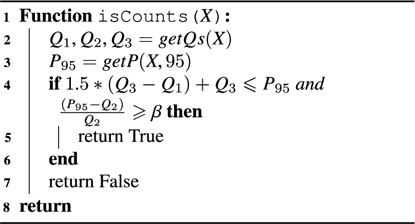
Detect counts type

6.4. The detection order

In our detection algorithm, we start by checking whether a column is ordinal because it is the most restrictive – it is the only one that checks for exact values. It tests whether the column is composed of natural numbers from 1 until n (n being the number of elements in the column).

The second step should check for equal digits (hierarchical, sequential) or categorical sub-types. However, the order here does not matter as categorical data contain a lot of duplicates, while sequential and hierarchical do not. We choose to check for categorical first. Then we check for the sequential sub-type as the hierarchical detection method checks if the numbers have the same number of digits and are not sequential. In the fourth step, we check if it is hierarchical. In the last step, we check if it is of the sub-type counts; otherwise, it will be of the sub-type other. Note that for the random sub-type, we do not have a detection method for it as mentioned earlier in this section. We show the detection order in Fig. 4.

Fig. 4.

Detection order of the numeric (sub-)types.

7. Model

In this section, we describe how we extract numeric values from a given knowledge graph. We use the extracted data to build a model that we use afterward to assign labels to numerical columns. This step (with the semantic labeling step in Section 8) corresponds to the “LABEL DETECTION” box in Fig. 1.

7.1. Data extraction

In this step, we extract the numeric values from the knowledge graph. To extract numeric properties from the knowledge graph, we use the following SPARQL query with a class URI. This will get all the properties for a given class.

Then, for each property, we check whether more than 50% of the values (which are known as objects) are numeric. If so, then we consider this property as a numeric property which will be used with its values to build the model.

7.2. Model construction

Before we build the model, we first need to detect the sub-types of the numbers for each property for the corresponding class. The model for each class is in the format shown in Table 2.

Table 2

Model features

Property URI	Numeric Type/Sub-type	Features
…/military-service-number	sequential	95000,…
…/height	other	192.4,…
…	…	…

Next, we show the different model construction methods for each numeric (sub-)type. We summarize the features for each sub-type in Table 3.

Table 3

Labeling features per sub-type

Type	Sub-type	Features
nominal	sequential	trimean, tstd
nominal	categorical	# categories∗, % categories†
ratio-interval	counts	trimean, tstd
ratio-interval	other	trimean, tstd

∗ The number of categories.

† The percentages of each category.

7.2.1. Nominal

The features used to build the model depend on whether the numbers are sequential, hierarchical, or categorical. We show how we compute features depending on different kinds of nominal numbers.

For the sequential kind, we use the trimean, which is more resistant to outliers than the mean [31]. We show the formula here: $$\begin{array}{}\text{(3)}& \mathit{trimean}={\displaystyle \frac{\mathit{Q}1+2\ast \mathit{Q}2+\mathit{Q}3}{4}}\end{array}$$

We also use the standard deviation with the trimean instead of the mean. We refer to the standard deviation with the trimean as tstd.

For the categorical sub-type, we use the number of unique numbers (the number of categories) followed by the percentages for each category ordered ascendingly.

Matching hierarchical data type with a numeric property from the knowledge graph is complex. If we know the different sections and which digits represent them, we would be able to do more,20

²⁰

E.g., treating each section differently or treating each section as a dimension.

but this is not the case, and hence we will not annotate them.

For the random sub-type, we ignore it because it is impossible to annotate such kind without extra evidence or elimination of other kinds, as it is random by definition.

7.2.2. Ordinal

This kind of data is common in tabular data, but we found that it is very limited in knowledge graphs, which makes sense as such ordering usually done with some filtering (e.g., the rank of runners in a competition A) hence, ordinal numbers are ignored.

7.2.3. Ratio and interval

We can distinguish the counts sub-type from the other sub-type as they have different aspects that can be exploited to annotate numeric columns.

Raw values of counts as-is are typically hard to understand and analyze [16,31]. Annotating such data by machines is also difficult as the probability distribution or the numbers (counts) alone does not provide enough evidence to distinguish the data [16,31]. Exact match will not be a solution as a single difference in counts (e.g., the data for the same events from a different year or reported by a different person) could be very close but not exactly the same.

Nonetheless, exploratory data analysis techniques may help us here. Although they are generally meant to be used by humans to explore the data, we intend to automate this process. So, we transform the data to help us in understanding it; exploratory data analysis experts use square root ( $\sqrt{\mathit{X}}$ ) and logs ( $log\mathit{X}$ ) to analyze the data; such transformation of data is referred to as “re-expression” of the data [16,31]. Logs generally make the results too close while square roots tend to be a good balance between the logs and the raw values [31]; hence, we transform the raw data using the square root. After that, we use the trimean Eq. (3) and the trimean-standard-deviation (tstd).

For the sub-type other, we use the trimean [31] Eq. (3) and (tstd).

The use of trimean and tstd instead of the mean and the standard deviation reduces the effects of long-tailed distributions in the input data and the values of the numeric properties in the knowledge graph.

8. Semantic labeling

In this section, we discuss the process of semantic labeling for the different types of numeric data, where we treat each type differently to maximize accuracy. We introduce different features specific to each sub-type.

For the labeling task, we use the fuzzy c-means clustering technique [3]. We can divide it into two steps: the first one is computing the centers of the clusters; the second step is the classification (to assign semantic labels). Note that in the classical fuzzy c-means, it computes the cluster centers based on the data points minimizing the total error. In our case, we compute the centers of the clusters by computing the features of the numeric properties extracted from the knowledge graph (Section 7). After that, we use the input data of the numeric column and compute the features, which is used to look for the closest cluster. As this is fuzzy clustering, it will belong to multiple clusters shown with a percentage value for each cluster.

8.1. Centroids

In contrast to classical fuzzy c-means [3], we compute the clusters centers – which are also known as centroids – using the list of features presented in Section 7. Each numeric property extracted from the knowledge graph has a separate centroid. The value of each centroid is the set of features of the corresponding numeric property.

The reason we compute the centroids that way is that we already know the clusters that correspond to the numeric properties, while in the classical fuzzy c-means, the clusters are not known and need to be discovered by the algorithm.

8.2. Classification

Given a collection of numbers as an input (a numeric column), we detect the (sub-)type. Then, we retrieve a corresponding model (a model with the same class), and we strip it to include only the numeric properties that match the detected sub-type. Next, we compute the features of the input as in Section 7.

The computed features are then used as new data points. As the features are comma-separated, each value will represent a dimension (see Table 2 and 3). For each data point – which are the features computed for a given numeric column – the membership vector is computed as in Eq. (4)21

²¹

This equation was introduced by Bezdek et al. [3] to compute the membership.

with fuzziness ( $\mathit{m}=2$ ) as suggested by Bezdek et al. [3]. We explain the variables in Table 4. The membership vector indicates the percentage of belonging of a given column to each of the clusters (numeric properties) in the model. $$\begin{array}{ll}\hfill & {\mathit{u}}_{\mathit{i}\mathit{k}}={\mathrm{\left(}{\displaystyle \sum }_{\mathit{j}=1}^{\mathit{c}}{\mathrm{\left(}{\displaystyle \frac{{\mathit{d}}_{\mathit{i}\mathit{k}}}{{\mathit{d}}_{\mathit{j}\mathit{k}}}}\mathrm{\right)}}^{2\mathrm{/}\mathrm{(}\mathit{m}-1\mathrm{)}}\mathrm{\right)}}^{-1}\\ \text{(4)}& \hfill & \forall \mathit{k}\mathrm{,}\mathit{i}:1⩽\mathit{k}⩽\mathit{N};1⩽\mathit{i}⩽\mathit{c}\end{array}$$

For example, if we have three clusters: $\mathit{dbp}\text{:}\mathit{height}$ , $\mathit{dbp}\text{:}\mathit{weight}$ , and $\mathit{dbp}\text{:}\mathit{waist}$ , a membership vector for a numeric column can be something like this $⟨0.15\mathrm{,}0.80\mathrm{,}0.05⟩$ . This means that the given column belongs 15% to $\mathit{dbp}\text{:}\mathit{height}$ cluster, 80% to $\mathit{dbp}\text{:}\mathit{weight}$ cluster, and 5% to $\mathit{dbp}\text{:}\mathit{waist}$ cluster. An output of the classification is the membership vector. For practical reasons, we order the results in descending order with the corresponding cluster and the membership vector as in Table 5. Note that the sum of the membership values for a given data point should be 1.

Table 4

Notation

Notation	Meaning
m	weighting exponent to control fuzziness
${\mathit{d}}_{\mathit{i}\mathit{k}}$	the distance between a datapoint k and a cluster center i
N	the number of data points
${\mathit{y}}_{\mathit{k}}$	the data point value at index k
c	number of clusters
${\mathit{v}}_{\mathit{i}}$	cluster at index i
${\mathit{u}}_{\mathit{i}\mathit{k}}$	the membership value of a data point at index k to cluster i

Table 5

Membership vector example

Cluster	Membership
$\mathit{dbp}:\mathit{weight}$	0.8
$\mathit{dbp}:\mathit{height}$	0.15
$\mathit{dbp}:\mathit{waist}$	0.5

9. Evaluation

In this section, we evaluate our hypothesis that detecting and treating numeric values differently based on the type of numeric values would results in a higher F1 score than using a general technique (in which different types of numbers are treated uniformly).

We define the set of experiments to evaluate our hypothesis; we describe the data we use, report the results of the experiments, and we conclude with the discussion of the results.

Table 6

Typology detection and labeling

Type	Sub-type	Detect	Label
Nominal	Sequential	yes	yes
Nominal	Hierarchical	yes	no
Nominal	Categorical	yes	yes
Nominal	Random	no	no
Ordinal	–	yes	no
Ratio-Interval	Counts	yes	yes
Ratio-Interval	Other	yes	yes

9.1. Experiment

As we are dealing with different types of numbers, we divide the input data for each (sub-)type: sequential, hierarchical, categorical, ordinal, counts, and other. We do this manually, and then we apply the detection methods we reported earlier in this paper. This is done to measure the performance of our detection methods. Then, taking into account the knowledge that we have about the (sub-)types of numbers, we apply the labeling methods and report the precision, recall, and F1 scores. The result of the detection is a type (e.g., nominal) and a sub-type (e.g., sequential). For the labeling, the output is the URI of the property matched to the numeric column that our algorithm determines to be the most probable. The source code of the experiment and the data are published [2] (also available on GitHub22

²²

https://github.com/oeg-upm/ttla

). It also includes the manual annotations and the (sub-)types for each of the numeric columns.23

²³

The manual annotation and assignment of the (sub-)types have been done by one of the authors, and the process took around two working days.

We summarize the (sub-)types that we are detecting and labeling in Table 6 with “yes” for the (sub-)types that we can detect or label and “no” for the ones we do not predict.

In order to compute precision we divide the number of correct prediction by the overall number of the predicted ones Eq. (5). For the recall, we divide the number of correctly predicted over the total number of the same type and sub-type Eq. (6). The final performance measure is the F1 score, which is calculated as shown in Eq. (7). These performance measures are used for both the detection and labeling experiments. $$\begin{array}{}\text{(5)}& \hfill & \mathit{precision}={\displaystyle \frac{\mathrm{\#}\mathit{correct}}{\mathrm{\#}\mathit{correct}+\mathrm{\#}\mathit{incorrect}}}\mathrm{,}\text{(6)}& \hfill & \mathit{recall}={\displaystyle \frac{\mathrm{\#}\mathit{correct}}{\mathrm{\#}\mathit{correct}+\mathrm{\#}\mathit{notfound}}}\mathrm{,}\text{(7)}& \hfill & \mathit{F}1={\displaystyle \frac{2\ast \mathit{precision}\ast \mathit{recall}}{\mathit{precision}+\mathit{recall}}}\end{array}$$

9.2. Data

We use the T2Dv2 dataset [25]: the only benchmark that we found in the literature that has different types of numeric columns. Ritze et al. [23] published this benchmark due to the lack of publicly annotated datasets, and the use of their benchmark started to become the de facto standard [1,7,20,23,24]. Nonetheless, we could not compare with other approaches because none of them (according to our knowledge) reported the scores of semantic labeling of numeric properties similarly. For this reason, we compare this work with our previous approach.

We use 124 numerical columns from that dataset that we were able to understand and for which we find a corresponding property in DBpedia. We show the typology found in the dataset in Table 7. We can see that the majority of columns belong to the type ratio-interval. The count type takes close to 0.4 of the total number of numerical columns. This has been reported in our previous paper [1] when talking about long-tailed distributions, which often caused by the data being condensed in one of the sides far from the mean. This was the primary cause of incorrect labeling in that work. We also notice here that we have a type called Year, which is not mentioned in the background nor in the typology that we adopt. This is due to its unique properties. The type Year is confusing as it can be thought of as a simple count from the birth of Jesus until a given moment. This could also be thought of as a nominal since it is often used to tag and name things produced, created, or occurred in a year without any regard for the counting aspect. Since it can be compared, some might argue that it is not nominal (nominal does not encompass the greater or less than operator [28]). Due to that, we will be ignoring it in our experiments.

Table 7

Typology in T2Dv2 dataset

Numeric Type	Sub-type	Percentage
Nominal	Sequential	0.008
Nominal	Hierarchical	0.0
Nominal	Categorical	0.0
Nominal	Random	0.048
Nominal	combined	0.056
Ordinal	–	0.04
Ratio-Interval	Count	0.387
Ratio-Interval	Other	0.234
Ratio-Interval	combined	0.621
Year	–	0.282

9.3. Results and discussion

9.3.1. Typology detection

We first report the scores for the detection of the typology for each of the numeric columns in Table 8. For the sequential, we found that there is only one column, and we got it wrong. The reason is the noise; the file contains multiple tables with headers located below each other, which does not make the column look like an actual sequence (it looks like a subset of different columns merged together into a single column). From the T2Dv2 benchmark, we did not find any hierarchical or categorical columns hence the N/A in the table. For the ordinal, we got high precision and recall applying a simple function. For the counts, we reached a precision score of approximately 0.8 and a similar recall. We inspected the wrongly detected ones, and we saw that they do not look like counts. Counts tend to have a high variance as the number increases (so differences increase as mentioned in Section 6), which was not the case in a couple of the columns that were wrongly detected. For the last type, it is when the data do not match any of the other sub-types, as mentioned in Section 6, so there is no specific detection algorithm for it.

Table 8

Typology detection scores

Numeric Type	Sub-type	Precision	Recall	F1
Nominal	Sequential	0.0	0.0	N/A
Nominal	Hierarchical	N/A	N/A	N/A
Nominal	Categorical	N/A	N/A	N/A
Nominal	Random	N/A	N/A	N/A
Ordinal	–	0.8	1.0	0.889
Ratio-Interval	Count	0.792	0.809	0.8
Ratio-Interval	Other	0.552	0.516	0.533

Table 9

Typology labeling scores

k	Numeric Type	Sub-type	Precision@k	Recall@k	F1@k
1	Nominal	Sequential	1.0	1.0	1.0
	Ratio-Interval	Count	0.822	0.949	0.881
	Ratio-Interval	Other	0.357	0.588	0.444
	All	–	0.649	0.842	0.733
3	Nominal	Sequential	1.0	1.0	1.0
	Ratio-Interval	Count	0.956	0.956	0.956
	Ratio-Interval	Other	0.893	0.781	0.833
	All	–	0.932	0.885	0.908
5	Nominal	Sequential	1.0	1.0	1.0
	Ratio-Interval	Count	1.0	0.957	0.978
	Ratio-Interval	Other	0.929	0.788	0.852
	All	–	0.973	0.889	0.929
10	Nominal	Sequential	1.0	1.0	1.0
	Ratio-Interval	Count	1.0	0.957	0.978
	Ratio-Interval	Other	1.0	0.8	0.889
	All	–	1.0	0.892	0.943

9.3.2. Semantic labeling

We report the precision, recall, and the F1 score for the semantic labeling experiment in Table 9. We do that for different values of k, taking the top k properties that are the most probable. For $\mathit{k}=1$ (taking into account only the top suggested property), the resulted recall is high (⩾ 0.8), while the precision is not as high ( $\mathrm{<}0.7$ ). Looking closely at the type with the lowest precision, we found that it is the other sub-type; we were not expecting the precision of it to be low.

We inspected the wrongly labeled properties and found that some are due to being labeled to knowledge graph specific/internal properties (e.g., dbo:wikiPageID) or wrong type detection. For example, the type of dbp:areaOfCatchment is wrongly detected as of sub-type counts when building the model (while it should have been other). Also, a couple of them wrongly point to properties related to years (e.g., dbp:yearLeader, dbo:eruptionYear). We found that years are one of the most difficult to work with, relying only on the values [1,30]. This could also be improved by having a better type detection, but may not prevent wrongly assigning year-related properties if the used typology does not have a (sub-)type year.

Not only the sub-type other has wrongly labeled properties, but also other types have mislabeled properties. We scrutinize and found that there are properties that are wrong in the knowledge graph. For example, the dbp:iosNumber of a dbo:Currency is labeled as dbp:width; we looked it up and found that there is nothing called the width of a currency. Looking at the values, they look similar to the values of dbp:iosNumber, so it makes sense why it was confused with it.

As the value of k increases and takes more properties into account, we notice the significant score increase, especially for the precision of the sub-type other; it rises from 0.357 to 0.893. This means that those correct properties are still in the top suggested ones for the most part, and the precision increase as we increase the value of k.

We have carefully checked the result for recall for the sub-type sequential. This may be misleading because there was only one column with that type, and the algorithm got it correctly, so the two possible outcomes were 0 or 1. We did not include results of the (sub-)types: hierarchical, categorical, random, ordinal. This is due to the lack of these types in either the input dataset or the knowledge graph. An exception to that is sub-type random; the reason is that we do not have a way to detect a such (sub-)type. As a result, the sub-type random is reported with the sub-type other (combined).

Table 10

Labeling scores of FCM and TTLA approaches

k	Approach	Precision@k	Recall@k	F1@k
1	TTLA	0.649	0.842	0.733
	FCM	0.34	1.0	0.51
	Random	0.0004	1.0*	0.0008†
3	TTLA	0.932	0.885	0.908
	FCM	0.55	1.0	0.71
	Random	0.0012	1.0*	0.0024†
5	TTLA	0.973	0.889	0.929
	FCM	0.83	1.0	0.91
	Random	0.002	1.0*	0.004†
10	TTLA	1.0	0.892	0.943
	FCM	0.91	1.0	0.95
	Random	0.004	1.0*	0.008†

∗ We assume here that all possible properties will be returned.

† The F1 score is computed under the assumption that the recall is 1.

We compare our approach with our previous work [1] as we did not find any other approach reporting the classification of numeric columns separately for the only two publicly available tabular datasets with numeric columns that we found. We denote our approach in Table 10 with TTLA (which stands for Tabular Typology-based LAbeling) and our previous approach with FCM as denoted in the other paper. We also include the scores of getting a correct property randomly from [1]. The scores of our approach (TTLA) for $\mathit{k}=1$ achieve twice the precision as the previous work (FCM). TTLA continues to out-perform FCM as we increase k. For high values of k, FCM might out-perform our typology-based semantic labeling approach as the previous FCM approach reports all possible properties. We can see a clear significant improvement of the precision of the TTLA compared to the old FCM approach. The recall is not reported in the previous work, so we put the sign − in the corresponding cell, and we report the recall to allow comparison in future work.

10. Conclusion and future work

In this paper, we introduced a typology of numeric data to improve the semantic labeling performance. We showed that taking into account this typology yields better performance for semantic labeling. We also found out that there are (sub-)types that are under-represented in the existing benchmarks (such as hierarchical and categorical).

As for the future work, we plan to extend the benchmark to include the under-represented (sub-)types. We also would like to explore the idea of having the sub-types as part of the features and use it to reduce the effect of the incorrect detection of (sub-)types.