Continuous top-k approximated join of streaming and evolving distributed data

Abstract

Continuously finding the most relevant (shortly, top-k) answer of a query that joins streaming and distributed data is getting a growing attention. In recent years, this is in particular happening in Social Media and IoT. It is well known that, in those settings, remaining reactive can be challenging, because accessing the distributed data can be highly time consuming as well as rate-limited. In this paper, we investigate the problem of continuous top-k query evaluation over a data stream joined with a distributed dataset in even a more extreme situation: the distributed data evolves. We propose the Topk+N algorithm and the AcquaTop framework. They keep up to date a local replica of the distributed dataset and guarantees reactiveness by construction, but to do so they may need to approximate the result. Therefore, we propose two maintenance policies to update the replica: the Top Selection Maintenance (AT-TSM) policy maximizes the relevancy, while the Border Selection Maintenance (AT-BSM) policy maximizes the accuracy of the top-k result. We contribute a theoretical proof of the correctness of Topk+N algorithm and we study its complexity. Moreover, we provide empirical evidence that the proposed policies within AcquaTop framework produce more relevant and accurate results than the state of the art.

1. Introduction

1.1. Motivation

Many modern applications require to combine highly dynamic data streams with distributed data, which evolves, to continuously answer queries in a reactive way.1

¹

A program is reactive if it maintains a continuous interaction with its environment, but at a speed which is determined by the environment, not by the program itself [4]. Real-time programs are reactive, but reactive programs can be non real-time as far as they provide result in time to successfully interact with the environment.

Consider the following two examples in Social Media and industrial IoT.

In social content marketing, advertisement agencies may want to continuously detect emerging influential Social Network users in order to ask them to endorse their commercials. To do so they monitor users’ mentions and number of followers in micro-posts across Social Networks. They need to select those users who are not already known to be the influencer, who are highly mentioned and whose number of followers grows fast. It is worth to note that (1) users’ mentions continuously arrive, (2) the number of followers may change in seconds, and (3) agencies have around a minute to detect them. Otherwise, the competitors may reach the emerging influencer sooner than them or the attention to the emerging influencer may drop. It is possible to formulate this information need as a continuous query of the form:

Return every minute the users who are not influencer, are mentioned the most and whose number of followers is growing the fastest.

In order to make the problem concrete, let us discuss how to implement this example using Twitter APIs. If we accessed Twitter firehose that streams all the tweets, we could obtain around 200,000 account mentions per minute. To obtain the number of followers of each mentioned account, we must use the REST service,2 ²

https://dev.twitter.com/rest/reference/get/users/lookup

which returns user descriptions for up to 100 users per request. So 2,000 requests per minute should return us the information we need to answer the query. Unfortunately, this naïve approach will fail to be reactive, as the REST service is rate limited, and each request takes around 0.1 s which is not enough to answer the query in one minute.

Let us present one more example, this time it is about manufacturing companies that use automation and instrumented their production lines with IoT sensor networks. In this setting, a production line consists of various machineries using different instruments. The companies track the usage of each instrument for maintenance purposes, and store the information in their Enterprise Resource Planning (ERP) systems that are not in the production sites. The IoT sensor networks in those companies continuously track the environmental conditions such as temperature, pressure, vibration, etc, and stream out them using IoT protocols such as MQTT.3 ³

Message Queuing Telemetry Transport (MQTT) is an extremely lightweight publish-subscribe-based messaging protocol. It is designed for connections with remote locations where a small code footprint is required and/or network bandwidth is limited.

A common usage of all this information is the reactive detection of the environmental condition that can affect the quality of the products. For example, to check (directly on the production site) the effects of vibration on the quality of the product, it is possible to formulate a continuous query such as:

Return every minute the list of products made with instruments that are the least recently maintained and are mounted on machines that show the highest vibrations.

As in the Social Media scenario, answering this query in a reactive manner is challenging since it joins thousands of observations per seconds on the MQTT stream with the information stored in the ERP. If, as it is often the case, the network between the production line and the ERP has a latency of 100 ms, it may be impossible to perform the entire join.

However, one may wonder if it is really necessary to perform the entire join to answer those two information needs introduced above. They clearly focus only on the top results. Indeed, the state of the art includes two families of partial solutions to this problem. On the one hand, the database community studied continuous top-k queries over the data streams [40] that can handle massive data streams focusing only on the top-k answer but ignoring the join with evolving distributed datasets. On the other hand, the Semantic Web community studied approximate continuous joining of RDF streams and dynamic linked data sets [10] which is reactive by design but it is not optimized for top-k queries.

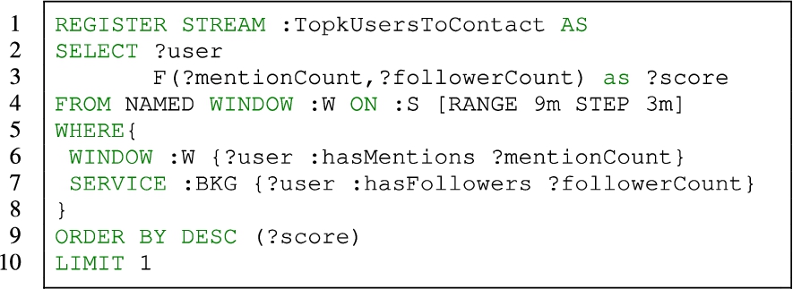
More specifically, the Semantic Web community showed that RDF Stream Processing (RSP) engines provide an adequate framework for continuous joining of the stream and the distributed data [11]. In this setting, distributed data is usually stored remotely or on the Web and accessible by using SPARQL query over SPARQL endpoints [8]. In order to access remote services, the query has to use federated SPAQRL syntax [35] which is supported by different query languages (e.g. C-SPARQL [3], SPARQL_stream [7], RSP-QL [13], and CQELS-QL [27]). For instance, Listing 1 shows a simplified version of the first example above formulated as a continuous RSP-QL top-k query using the syntax proposed in [12].

Listing 1.

Sketch of the query studied in the problem.

At each query evaluation, the WHERE clause at lines 5–8 is matched against the data in a window :W open on the data stream :S, on which the mentions of each user flows, and in the remote SPARQL service :BKG, which contains the number of followers for each user. Function F is a user-specified scoring function that computes the score of each user as the normalized sum of her mentions (?mentionCount) and her number of followers (?followerCount). The users are ordered by their scores, and the number of results is limited to 1. As a result this query returns the top-1 result for each evaluation.

Fig. 1.

The example that shows the objects in top-k result after join clause evaluation of windows ${\mathit{W}}_0$ , and ${\mathit{W}}_1$ .

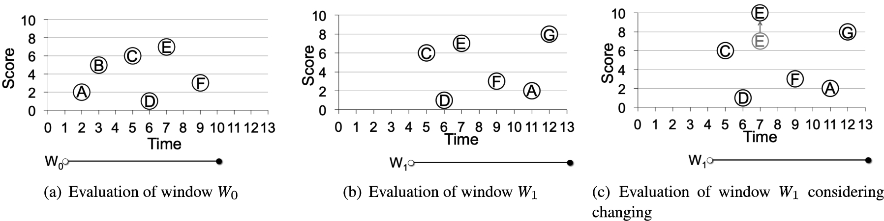
Figures 1(a), and 1(b) show a portion of a stream between time 0 and 13. The X axis shows the arriving time on the stream of the number of mentions of a certain user to the system, while the Y axis shows the score of the user computed after evaluating the join clause with the number of followers fetched from the distributed data. For the sake of clarity, we label each point in the Cartesian space with the ID of the user it refers to. This stream is observed through a window that has a length equal to 9 minutes and slides every 3 minutes. In particular, Fig. 1(a) shows the content of window ${\mathit{W}}_0$ that opens at 1 (excluded) and closes at 10. Figure 1(b) shows the next window ${\mathit{W}}_1$ after the sliding of 3 minutes. Each circle indicates the score of a user after the evaluation of the JOIN clause, but before the evaluation of the ORDER and LIMIT clauses.

During window ${\mathit{W}}_0$ users A, B, C, D, E, and F come to the system (Fig. 1(a)). When ${\mathit{W}}_0$ expired, users A and B go out of the result. Before the end of the window ${\mathit{W}}_1$ , user A arrives again and the new user G appears (Fig. 1(b)). Evaluating the query in Listing 1 gives us user E as the top-1 result for window ${\mathit{W}}_0$ and user G as top-1 result for window ${\mathit{W}}_1$ .

However, changes in the number of followers of a user in the distributed data can alter the score of a user between subsequent query evaluations, and this can affect the result. For example, in Fig. 1(c), between the evaluation time of windows ${\mathit{W}}_0$ , and ${\mathit{W}}_1$ , the score of user E changes from 7 to 10 (due to an increment in the number of followers in the distributed data). Considering the new score of user E in the evaluation of window ${\mathit{W}}_1$ , the top-1 result is no longer user G, but it is user E.

As we mention above, while RSP-QL allows encoding top-k queries, state-of-the-art RSP engines are not optimized for such a type of queries and they would recompute the result from scratch as explained in [32,34]. This put them at risk of losing reactiveness. In order to handle this situation, in this paper we investigate the following research question: How can we continuously, if needed approximately, optimize a top-k join of a stream and a distributed dataset which may change between consecutive evaluations, while guaranteeing the reactiveness of the system?

In continuous top-k query answering, it is well known that recomputing the top-k result from scratch at every evaluation is a major performance bottleneck. In 2006, Mouratidis et al. [32] were the first to solve this problem proposing an incremental query evaluation approach that uses a data structure known as k-skyband and an algorithm to precompute the future results in order to reduce the probability of recomputing the top-k results from scratch. Few years after, in 2011, Di Yang et al. [40] completely removed this performance bottleneck designing MinTopk algorithm which answers a top-k query without any recomputation of top-k results from scratch. The approach memorizes only the minimal subset of the streaming data which is necessary and efficient for query evaluation and discards the rest. The authors also showed the optimality of the proposed algorithm in both CPU and memory utilization for continuous top-k monitoring. Unfortunately, MinTopk algorithm cannot be applied to queries that join streaming data with distributed data, especially when the distributed data evolves.

A solution to this problem can be found in the RSP state-of-the-art, where a few years ago S. Dehghanzadeh et al. [10] noticed that high latency and limitation of the access rate can put the RSP engine at risk of losing reactiveness and addressed this problem, using a local replica of the distributed dataset (shortly named ACQUA in the remainder of this paper). The authors defined the notion of refresh budget to limit the number of remote accesses to the distributed dataset for updating the local replica, and guaranteeing by construction the reactiveness of the system. However, if the refresh budget is not enough to refresh all the data in the replica, some of the data items become stale, and the query result can contain errors. The authors showed that expertly designed maintenance policies can update the local replica in order to reduce the number of errors and approximate the correct result. Unfortunately, also this approach is not optimized for top-k queries.

1.2. Contributions

In this paper, we extend the state-of-the-art approach for top-k query evaluation [40], focusing on 1:1 joins,4

⁴

While restricting the contribution to 1:1 joins may appear a serious limit, the readers should notice that the two motivational examples above require exactly a 1:1 join. The social media marketing example requires to look up fully hydrated user profiles of those mentioned in the tweets. The manufacturing example requires to look up the context of each observation measured by the IoT sensors.

and considering distributed dataset that has changes during the evaluation. Our contributions are highlighted in boldface in the following paragraphs.

As a first solution, we assume that all changes are pushed from the distributed data to the engine that continuously evaluates the query. We extend the data structure proposed in [40] and introduce Super-MTK $\mathbf{+}$ N list that keeps the necessary and sufficient data for top-k query evaluation. The proposed data structure can handle changes in distributed data while minimizing the memory usage. However, MinTopk algorithm [40] assumed distinctive arrival of data, so to handle the changes pushed from the distributed dataset, we have to modify it to support indistinct arrival of data. Indeed, in the example, user E is already in the window when her number of followers changes and so does the score. The proposed Topk $\mathbf{+}$ N algorithm considers the changed data items as new arrivals with new scores. The proposed Super-MTK+N list keeps the data items that have a higher probability to appear in the result of query evaluation. Keeping N additional items in the top-k result of each evaluation in the Super-MTK+N list lets Topk+N algorithm to handle the changes in the distributed dataset, and provide a relevant answer.

This first solution works in a data center, where the entire infrastructure is under control, network latency is low and bandwidth is large, but it may not work on the Web, which is decentralized and where we can frequently experience high network latency, low bandwidth and even rate-limited access. In this setting, the engine, which continuously evaluates the query, has to pull the changes form the distributed data. Therefore, considering the architectural approach presented in [10] as a guideline, we propose a second solution, named AcquaTop framework, that keeps a local replica of the distributed data and updates a part of it according to a given refresh policy before every evaluation. Notably, when we have got enough refresh budget to update all the stale elements in the replica the proposed approach is exact, but when we have not, we might have some errors in the result.

In order to approximate as much as possible the correct answer in this extreme situation, we propose two maintenance policies to update the replica using AcquaTop algorithm. They are specifically tailored to top-k approximated join. The Top Selection Maintenance (AT-TSM) policy maximizes the relevance, i.e., minimizes the difference between the order of the answers in the approximate top-k result and the correct order. The Border Selection Maintenance (AT-BSM) policy, instead, maximizes the accuracy of the top-k result, i.e., it tries to get all the top-k answers in the result, but it may fail to order results correctly.

The remainder of the paper is organized as follows. In Section 2, we formalize the problem and introduce the relevant background information. In Section 3, we introduce state-of-the-art works. Section 4, and 5 present our proposed solutions for top-k query evaluation over stream and dynamic distributed dataset. Section 6 discusses the experimental setting and the research hypotheses, reports on the evaluation of the proposed approach, and highlights the practical insights we gathered. In Section 7, we review the related work regarding our contributions and, finally, Section 8 concludes and presents future works.

2. Problem definition

This section, first, introduces the background necessary to understand the paper (Section 2.1) and, then, proposes a formal problem statement (Section 2.2).

2.1. Preliminaries

In this section, we present two preliminary contents: RSP-QL semantics, which is important for precisely formalizing the problem in Section 2.2, and the metrics, which we use to evaluate the quality of the answers in the result.

2.1.1. RSP-QL semantic

RDF Stream Processing (RSP) [14] extends the RDF data model and query model considering the temporal dimension of data and the evolution of data over time. In the following, we introduce the definitions of RSP-QL [13].

An RSP-QL query is defined by a quadruple $⟨\mathit{\text{ET}}\mathrm{,}\mathit{\text{SDS}}\mathrm{,}\mathit{\text{SE}}\mathrm{,}\mathit{\text{QF}}⟩$ , where ET is a sequence of evaluation time instants, SDS is an RSP-QL dataset, SE is an RSP-QL algebraic expression, and QF is a query form.

In order to define SDS, we need first to introduce the concepts of time, RDF stream and window over an RDF stream that creates RDF graphs by extracting relevant portions of the stream.

Definition 2.1.

Time. The time T is an infinite, discrete, ordered sequence of time instants $\mathrm{(}{\mathit{t}}_1\mathrm{,}{\mathit{t}}_2\mathrm{,}\dots \mathrm{)}$ , where ${\mathit{t}}_{\mathit{i}}\in \mathbb{N}$ .

Definition 2.2.

Evaluation Time. The Evaluation Time $\mathit{ET}\subseteq \mathit{T}$ is a sequence of time instants at which the evaluation occurs. It is not practical to give ET explicitly, so normally ET is derived from an evaluation policy (see [13]).

Definition 2.3.

RDF Statement. An RDF statement is a triple $\mathrm{(}\mathit{s}\mathrm{,}\mathit{p}\mathrm{,}\mathit{o}\mathrm{)}\in \mathrm{(}\mathit{I}\cup \mathit{B}\mathrm{)}\times \mathrm{(}\mathit{I}\mathrm{)}\times \mathrm{(}\mathit{I}\cup \mathit{B}\cup \mathit{L}\mathrm{)}$ , where I is the set of IRIs, B is the set of blank nodes and L is the set of literals [26].

Definition 2.4.

RDF Stream. An RDF stream S is a potentially unbounded sequence of timestamped data items $\mathrm{(}{\mathit{d}}_{\mathit{i}}\mathrm{,}{\mathit{t}}_{\mathit{i}}\mathrm{)}$ : $$\begin{array}{c}\mathit{S}=\mathrm{(}{\mathit{d}}_1\mathrm{,}{\mathit{t}}_1\mathrm{)}\mathrm{,}\mathrm{(}{\mathit{d}}_2\mathrm{,}{\mathit{t}}_2\mathrm{)}\mathrm{,}\dots \mathrm{,}\mathrm{(}{\mathit{d}}_{\mathit{n}}\mathrm{,}{\mathit{t}}_{\mathit{n}}\mathrm{)}\mathrm{,}\dots \mathrm{,}\end{array}$$ where ${\mathit{d}}_{\mathit{i}}$ is an RDF statement, ${\mathit{t}}_{\mathit{i}}\in \mathit{T}$ the associated time instant, and for each data item ${\mathit{d}}_{\mathit{i}}$ , it holds ${\mathit{t}}_{\mathit{i}}⩽{\mathit{t}}_{\mathit{i}+1}$ (i.e., the time instants are non-decreasing).

Beside RDF streams, it is possible to have static or quasi-static data, which can be stored in RDF repositories or embedded in Web pages. For that data, the time dimension of SDS can be defined through the notions of time-varying and instantaneous graphs. The time-varying graph $\bar{\mathit{G}}$ is a function that maps time instants to RDF graphs and instantaneous graph $\bar{\mathit{G}}\mathrm{(}\mathit{t}\mathrm{)}$ is the value of the graph at a fixed time instant t.

Definition 2.5.

Time-based Window. A time-based window $\mathit{W}\mathrm{(}\mathit{S}\mathrm{)}$ is a set of RDF statements extracted from a stream S, and defined through opening and closing time instance (i.e., o, and c time instance) where $\mathit{W}\mathrm{(}\mathit{S}\mathrm{)}=\{\mathit{d}|\mathrm{(}\mathit{d}\mathrm{,}\mathit{t}\mathrm{)}\in \mathit{S}\mathrm{,}\mathit{t}\in \mathrm{(}\mathit{o}\mathrm{,}\mathit{c}]\}$ .

Definition 2.6.

Time-based Sliding Window. A time-based sliding window operator $\mathbb{W}$ [13], takes an RDF stream S as input and produces a time-varying graph ${\mathit{G}}_{\mathbb{W}}$ . $\mathbb{W}$ is defined through three parameters: ω – its width –, β – its slide –, and ${\mathit{t}}^0$ – the time stamp on which $\mathbb{W}$ starts to operate.

Operator $\mathbb{W}$ generates a sequence of time-based windows. Given two consecutive windows ${\mathit{W}}_{\mathit{i}}$ , ${\mathit{W}}_{\mathit{j}}$ defined in $\mathrm{(}{\mathit{o}}_{\mathit{i}}\mathrm{,}{\mathit{c}}_{\mathit{i}}]$ and $\mathrm{(}{\mathit{o}}_{\mathit{j}}\mathrm{,}{\mathit{c}}_{\mathit{j}}]$ , respectively, it holds: ${\mathit{o}}_{\mathit{i}}={\mathit{t}}_0+\mathit{i}\ast \mathit{\omega }$ , ${\mathit{c}}_{\mathit{i}}-{\mathit{o}}_{\mathit{i}}={\mathit{c}}_{\mathit{j}}-{\mathit{o}}_{\mathit{j}}=\mathit{\omega }$ , and ${\mathit{o}}_{\mathit{j}}-{\mathit{o}}_{\mathit{i}}=\mathit{\beta }$ . The sliding window could be count- or time-based [1].

Active windows are defined as all the windows that contain the current time in their duration. Current window is the window that closes in the current evaluation time. As stated in the beginning of this section, normally, evaluation times are derived from an evaluation policy. The evaluation times can be equal to the arrival times of objects, or can be equal to the closing time of each window. In this paper, we consider all the closing time of windows as evaluation times. Given current window ${\mathit{W}}_{\mathrm{cur}}$ , and next window ${\mathit{W}}_{\mathrm{nxt}}$ as two consecutive windows defined in $\mathrm{(}{\mathit{o}}_{\mathrm{cur}}\mathrm{,}{\mathit{c}}_{\mathrm{cur}}]$ and $\mathrm{(}{\mathit{o}}_{\mathrm{nxt}}\mathrm{,}{\mathit{c}}_{\mathrm{nxt}}]$ , respectively, we define current evaluation time as the closing time of current window, ${\mathit{c}}_{\mathrm{cur}}$ , and next evaluation time as the closing time of next window, ${\mathit{c}}_{\mathrm{nxt}}$ .

An RSP-QL dataset SDS is a set composed by one default time-varying graph ${\overline{\mathit{G}}}_0$ , a set of n time-varying named graphs $\{\mathrm{(}{\mathit{u}}_{\mathit{i}}\mathrm{,}{\overline{\mathit{G}}}_{\mathit{i}}\mathrm{)}\}$ , where ${\mathit{u}}_{\mathit{i}}\in \mathit{I}$ is the name of the element; and a set of m named time-varying graphs obtained by the application of time-based sliding windows over $\mathit{o}⩽\mathit{m}$ streams, $\mathrm{(}{\mathit{u}}_{\mathit{j}}\mathrm{,}{\mathbb{W}}_{\mathit{j}}\mathrm{(}{\mathit{S}}_{\mathit{k}}\mathrm{)}\mathrm{)}\}$ , where $\mathit{j}\in [1\mathrm{,}\mathit{m}]$ , and $\mathit{k}\in [1\mathrm{,}\mathit{o}]$ . It is possible to determine a set of instantaneous graphs and fixed windows for a fixed evaluation time instant, i.e. RDF graphs, and to use them as input data for the algebraic expression evaluation.

An algebraic expression SE is a streaming graph pattern which is the extension of a graph pattern expression defined by SPARQL. It is composed by operators mostly inspired by relational algebra, such as joins, unions and selections. In addition to the ones defined in SPARQL, RSP-QL adds a set of operators to transform the query result in an output stream. Considering the recursive definition of the graph pattern, streaming graph pattern expressions are recursively defined as follows [13]:

• a basic graph pattern (i.e. set of triple patterns $\mathrm{(}\mathit{s}\mathrm{,}\mathit{p}\mathrm{,}\mathit{o}\mathrm{)}\in \mathrm{(}\mathit{I}\cup \mathit{B}\cup \mathit{V}\mathrm{)}\times \mathrm{(}\mathit{I}\cup \mathit{V}\mathrm{)}\times \mathrm{(}\mathit{I}\cup \mathit{B}\cup \mathit{L}\cup \mathit{V}\mathrm{)}$ ) is a graph pattern;

• let P be a graph pattern and F a built-in condition, $\mathit{P}\mathit{\text{FILTER }}\mathit{F}$ is a graph pattern;

• let ${\mathit{P}}_1$ and ${\mathit{P}}_2$ be two graph patterns, ${\mathit{P}}_1\mathit{\text{UNION }}{\mathit{P}}_2$ , ${\mathit{P}}_1\mathit{\text{JOIN }}{\mathit{P}}_2$ and ${\mathit{P}}_1\mathit{\text{OPT }}{\mathit{P}}_2$ are graph patterns;

• let P be a graph pattern and $\mathit{u}\in \mathrm{(}\mathit{I}\cup \mathit{V}\mathrm{)}$ , the expressions $\mathit{\text{SERVICE }}\mathit{u}\mathit{P}$ , $\mathit{\text{GRAPH }}\mathit{u}\mathit{P}$ and $\mathit{\text{WINDOW }}\mathit{u}\mathit{P}$ are graph patterns.

RSP-QL query form QF is defined as in SPARQL (see Section 16 of SPARQL 1.1 W3C Recommendation5 ⁵

https://www.w3.org/TR/sparql11-query/#QueryForms

). The query form uses the solution mappings to form result sets or RDF graphs. There exist four query form: (i) SELECT which returns all or subset of the variables bound in a query pattern match, (ii) CONSTRUCT which returns an RDF graph, (iii) ASK which return a boolean that shows query pattern matches or not, and (iv) DESCRIBE which returns an RDF graph that describes the resources found.

As in SPARQL, the instantaneous evaluation of streaming graph pattern expressions produces sets of solution mappings. A solution mapping is a function that maps variables to RDF terms, i.e., $\mathit{\mu }:\mathit{V}\to \mathrm{(}\mathit{I}\cup \mathit{B}\cup \mathit{L}\mathrm{)}$ . $\mathit{\text{dom}}\mathrm{(}\mathit{\mu }\mathrm{)}$ denotes the subset of V where μ is defined. $\mathit{\mu }\mathrm{(}\mathit{x}\mathrm{)}$ indicates the RDF term resulting by applying the solution mapping to variable x [33].

Two solution mappings ${\mathit{\mu }}_1$ and ${\mathit{\mu }}_2$ are compatible ( ${\mathit{\mu }}_1\sim {\mathit{\mu }}_2$ ) if the two mappings assign the same value to each variable in $\mathit{\text{dom}}\mathrm{(}{\mathit{\mu }}_1\mathrm{)}\cap \mathit{\text{dom}}\mathrm{(}{\mathit{\mu }}_2\mathrm{)}$ (i.e., $\forall \mathit{x}\in \mathit{\text{dom}}\mathrm{(}{\mathit{\mu }}_1\mathrm{)}\cap \mathit{\text{dom}}\mathrm{(}{\mathit{\mu }}_2\mathrm{)}$ , ${\mathit{\mu }}_1\mathrm{(}\mathit{x}\mathrm{)}={\mathit{\mu }}_2\mathrm{(}\mathit{x}\mathrm{)}$ ).

Let now ${\mathrm{\Omega }}_1$ and ${\mathrm{\Omega }}_2$ be two sets of solution mappings, the join is defined as: $$\begin{array}{ll}\hfill & {\mathrm{\Omega }}_1\bowtie {\mathrm{\Omega }}_2\\ \hfill & =\{{\mathit{\mu }}_1\cup {\mathit{\mu }}_2|{\mathit{\mu }}_1\in {\mathrm{\Omega }}_1\mathrm{,}{\mathit{\mu }}_2\in {\mathrm{\Omega }}_2\mathrm{,}{\mathit{\mu }}_1\sim {\mathit{\mu }}_2\}\end{array}$$ Definition 2.7.

Top-k Continuous Query. A top-k Continuous RSP-QL query is a special type of RSP-QL query that for each evaluation time returns at most k results. Those k results are selected ordering the results of the algebraic expression SE according to a user-specified ranking function $\mathit{F}\mathrm{(}{\mathit{v}}_1\mathrm{,}\dots \mathrm{,}{\mathit{v}}_{\mathit{m}}\mathrm{)}$ , where ${\mathit{v}}_1\mathrm{,}\dots \mathrm{,}{\mathit{v}}_{\mathit{m}}$ are variables in SE. We name ${\mathit{v}}_1\mathrm{,}\dots \mathrm{,}{\mathit{v}}_{\mathit{m}}$ scoring variables. As normally done in top-k query literature, F is monotonic.

2.1.2. Metrics

Measuring the accuracy of top elements in the result is crucial for evaluating the quality of the approximation for the type of queries that we consider in this paper. Different criteria exist to measure this quality such as the precision at k, the accuracy at k, the normalized discounted cumulative gain ( $\mathit{nDCG}$ ), or the mean reciprocal rank (MRR) [5].

In the following, we introduce two metrics that we use in our experiments in order to compare the possibly approximated result of a query at time i, named $\mathit{\text{Ans}}\mathrm{(}{\mathit{Q}}_{\mathit{i}}\mathrm{)}$ , with certainly correct answers obtained from setting up an Oracle, named $\mathit{\text{Ans}}\mathrm{(}{\mathit{Oracle}}_{\mathit{i}}\mathrm{)}$ .

Discounted cumulative gain Discounted Cumulative Gain ( $\mathit{DCG}$ ) is widely used in information retrieval to measure relevancy (i.e., the quality of ranking).

There are two obvious facts in the evaluation of ranked result of a query: (i) The highly relevant items are more valuable comparing to others; and (ii) The higher the rank of a relevant item, the more valuable it is for the user [22]. The gain of each result set is computed by summing up the gains of the items in the result set, which is equal to their relevancies. In order to consider the ranked position of each item in the list, $\mathit{DCG}$ applies a discount factor, which reduces the gain of items with lower rank, as they are less valuable for user. $\mathit{DCG}$ at particular position k is defined as: $$\begin{array}{c}\mathit{DCG}@\mathit{k}={\displaystyle \sum }_{\mathit{i}=1}^{\mathit{k}}{\displaystyle \frac{2^{{\mathrm{rel}}_{\mathit{i}}}-1}{{log}_2\mathrm{(}\mathit{i}+1\mathrm{)}}}\end{array}$$ Where ${\mathrm{rel}}_{\mathit{i}}$ is the graded relevance of the result at position i.

In order to compare different result sets for various queries and positions, $\mathit{DCG}$ must be normalized across queries to do so. First, we produce the maximum possible $\mathit{DCG}$ through position k, which is called Ideal $\mathit{DCG}$ ( $\mathit{IDCG}$ ). This is done by sorting all relevant items by their relative relevance. Then, the normalized discounted cumulative gain ( $\mathit{nDCG}$ ), is computed as: $$\begin{array}{c}\mathit{nDCG}@\mathit{k}={\displaystyle \frac{\mathit{DCG}@\mathit{k}}{\mathit{IDCG}@\mathit{k}}}\end{array}$$

Precision If we focus on having all the correct answers in the result, the key feature of the top-k result is their correctness, while their ranks are less critical. In this case, we can use precision as metric. Precision in information retrieval computes the ratio between the correct instances in the result and all the retrieved instances. Considering the definition of precision as $\mathit{precision}=\frac{\mathit{t}\mathit{p}}{\mathit{t}\mathit{p}+\mathit{f}\mathit{p}}$ , where $\mathit{t}\mathit{p}$ is the number of true positive values, and $\mathit{f}\mathit{p}$ is the number of false positive ones, the precision at position k is defined as: $$\begin{array}{c}\mathit{precision}@\mathit{k}={\displaystyle \frac{\mathrm{\#}\text{positive instances in the result}}{\mathit{k}}}\end{array}$$ where the true positive value is equal to the number of positive instances in the top-k result, and the summation of true positive and false positive values are equal to k.

Fig. 2.

Algebraic expression.

To understand the difference between $\mathit{nDCG}@\mathit{k}$ and $\mathit{precision}@\mathit{k}$ , let us consider the following example. Assuming that we have got the following list of items as a correct answer of a query: $\{\mathit{A}\mathrm{,}\mathit{B}\mathrm{,}\mathit{C}\mathrm{,}\mathit{D}\mathrm{,}\mathit{E}\mathrm{,}\mathit{F}\}$ with relevancy respectively equal to $\{6\mathrm{,}5\mathrm{,}4\mathrm{,}3\mathrm{,}2\mathrm{,}1\}$ . Considering two top-3 answers: $\{\mathit{A}\mathrm{,}\mathit{D}\mathrm{,}\mathit{F}\}$ , and $\{\mathit{F}\mathrm{,}\mathit{C}\mathrm{,}\mathit{B}\}$ as case 1, and 2. In the first case, as item A with the highest relevancy is correctly ranked in the result, we expect a high value of $\mathit{nDCG}@3$ .

Considering $\{\mathit{A}\mathrm{,}\mathit{B}\mathrm{,}\mathit{C}\}$ as the correct result of the first case, the $\mathit{IDCG}$ is computed as follows: $$\begin{array}{l}\hfill \mathit{IDCG}={\displaystyle \frac{63}{1}}+{\displaystyle \frac{31}{1.585}}+{\displaystyle \frac{15}{2}}=90.06\end{array}$$ and $\mathit{nDCG}@3$ is computed as: $$\begin{array}{ll}\hfill \mathit{nDCG}@3& ={\displaystyle \frac{\mathit{DCG}}{\mathit{IDCG}}}\\ \hfill & ={\displaystyle \frac{63+4.42+0.5}{90.06}}=0.754\end{array}$$

The $\mathit{precision}@\mathit{k}$ is computed as: $$\begin{array}{l}\hfill \mathit{precision@}\mathit{3}={\displaystyle \frac{\mathit{t}\mathit{p}}{\mathit{k}}}={\displaystyle \frac{1}{3}}=0.333\end{array}$$

So, for the first case, $\mathit{nDCG}@3$ is equal to 0.754 while $\mathit{precision}@3$ is equal to 0.33, which shows that the result is more relevant and less accurate. Data item A, which is the most relevant item, is ranked in the correct place and the other answers are not the correct ones.

On the contrary, the second case contains more correct answers, so we expect a high value of $\mathit{precision}@3$ . For the second case, $\mathit{nDCG}@3$ is equal to 0.288 while $\mathit{precision}@3$ is equal to 0.667, which indicates that the result is more accurate and less relevant. There are 2 correct answers in the result, but comparing to the case 1, they are less relevant.

2.2. Problem statement

In this paper, we consider top-k continuous RSP-QL queries over a data stream $\mathcal{S}$ and a distributed dataset  $\mathcal{D}$ . We assume that: (i) there is a 1:1 join relationship between the data items in the data stream and those in the distributed dataset; (ii) the window, opened over the stream $\mathcal{S}$ , slides (i.e., $\mathit{\omega }\mathrm{>}\mathit{\beta }$ ); (iii) queries are evaluated when windows close and (iv) the distributed dataset can evolve between subsequent evaluations.

Moreover, the algebraic expression SE of this class of RSP-QL queries is defined as in Fig. 2(a), where:

• ${\mathit{P}}_{\mathcal{S}}$ , and ${\mathit{P}}_{\mathcal{D}}$ are graph patterns,

• ${\mathit{u}}_{\mathcal{S}}$ , and ${\mathit{u}}_{\mathcal{D}}$ identify the window on the RDF stream and the remote SPARQL endpoint,

• ${\mathit{\mu }}_{\mathcal{S}}$ is a solution mapping of the graph pattern $\mathit{\text{WINDOW }}{\mathit{u}}_{\mathcal{S}}{\mathit{P}}_{\mathcal{S}}$ ,

• ${\mathit{\mu }}_{\mathcal{D}}$ is a solution mapping of the graph pattern $\mathit{\text{SERVICE}}{\mathit{u}}_{\mathcal{D}}{\mathit{P}}_{\mathcal{D}}$ ,

• ${\mathit{x}}_{\mathcal{S}}$ , and ${\mathit{x}}_{\mathcal{D}}$ are scoring variables in mapping ${\mathit{\mu }}_{\mathcal{S}}$ and ${\mathit{\mu }}_{\mathcal{D}}$ ,

• ${\mathit{x}}_{\mathcal{J}}$ is a join variable in $\mathit{\text{dom}}\mathrm{(}{\mathit{\mu }}_{\mathit{S}}\mathrm{)}\cap \mathit{\text{dom}}\mathrm{(}{\mathit{\mu }}_{\mathit{D}}\mathrm{)}$ , and

• $\mathit{F}\mathrm{(}{\mathit{x}}_{\mathcal{S}}\mathrm{,}{\mathit{x}}_{\mathcal{D}}\mathrm{)}$ is a monotone scoring function, which generates the score and adds it to the solution mapping by using the EXTEND operator.6

  ⁶

  https://www.w3.org/TR/sparql11-query/#sparqlAlgebra

  For the sake of clarity, Fig. 2(b) illustrates the algebraic expression of the query in Listing 1. $?\mathit{user}$ : $\mathit{hasMentions}$   $?\mathit{mentionCount}$ , and $?\mathit{user}$ : $\mathit{hasFollowers}$   $?\mathit{followerCount}$ are the graph patterns respectively in the WINDOW and in the SERVICE clauses. $?\mathit{mentionCount}$ , and $?\mathit{followerCount}$ are the scoring variable, and $?\mathit{user}$ is the join variable. The scoring function F gets $?\mathit{mentionCount}$ , and $?\mathit{followerCount}$ as inputs and generates the score for each user. Once each solution mapping of the join is extended with a score, the solution mappings are ordered by their score and the top-k ones are reported as result.

  In the remainder of the paper, we focus our attention on the solution mappings ${\mathrm{\Omega }}_{\mathit{E}}$ of the EXTEND graph pattern where for each solution mapping ${\mathit{\mu }}_{\mathit{E}}\in {\mathrm{\Omega }}_{\mathit{E}}$ we have: $\mathit{\text{dom}}\mathrm{(}{\mathit{\mu }}_{\mathit{E}}\mathrm{)}=\mathit{\text{dom}}\mathrm{(}{\mathit{\mu }}_{\mathit{S}}\mathrm{)}\cup \mathit{\text{dom}}\mathrm{(}{\mathit{\mu }}_{\mathit{D}}\mathrm{)}\cup \{?\mathit{score}\}$ . Let us call Object O(id, score) one of such results, where the $\mathit{id}={\mathit{\mu }}_{\mathit{E}}\mathrm{(}{\mathit{x}}_{\mathcal{J}}\mathrm{)}$ , and the score $\mathit{O}.\mathit{\text{score}}$ is a real number computed by the scoring function $\mathit{F}\mathrm{(}{\mathit{\mu }}_{\mathit{E}}\mathrm{(}{\mathit{x}}_{\mathcal{S}}\mathrm{)}\mathrm{,}{\mathit{\mu }}_{\mathit{E}}\mathrm{(}{\mathit{x}}_{\mathcal{D}}\mathrm{)}\mathrm{)}$ . We denote $\mathit{O}.{\mathit{\text{score}}}_{\mathcal{S}}$ , and $\mathit{O}.{\mathit{\text{score}}}_{\mathcal{D}}$ the values coming from the streaming and the distributed data, respectively, i.e., $\mathit{O}.{\mathit{\text{score}}}_{\mathcal{S}}={\mathit{\mu }}_{\mathit{E}}\mathrm{(}{\mathit{x}}_{\mathcal{S}}\mathrm{)}$ , and $\mathit{O}.{\mathit{\text{score}}}_{\mathcal{D}}={\mathit{\mu }}_{\mathit{E}}\mathrm{(}{\mathit{x}}_{\mathcal{D}}\mathrm{)}$ .

  Let us, now, formalize the notion of changes in the distributed dataset that may occur between consecutive evaluations of the top-k query. Assuming ${\mathit{t}}^{\prime }$ and ${\mathit{t}}^{″}$ as two consecutive evaluation times (i.e. ${\mathit{t}}^{\prime }\mathrm{,}{\mathit{t}}^{″}\in \mathit{ET}$ , and $\nexists {\mathit{t}}^{‴}\in \mathit{ET}:{\mathit{t}}^{\prime }\mathrm{<}{\mathit{t}}^{‴}\mathrm{<}{\mathit{t}}^{″}$ ) the instantaneous graph ${\bar{\mathit{G}}}_{\mathit{d}}\mathrm{(}{\mathit{t}}^{\prime }\mathrm{)}$ in the distributed data differs from the instantaneous graphs ${\bar{\mathit{G}}}_{\mathit{d}}\mathrm{(}{\mathit{t}}^{″}\mathrm{)}$ .

  The changes between ${\bar{\mathit{G}}}_{\mathit{d}}\mathrm{(}{\mathit{t}}^{\prime }\mathrm{)}$ , and ${\bar{\mathit{G}}}_{\mathit{d}}\mathrm{(}{\mathit{t}}^{″}\mathrm{)}$ can affect the result of the top-k query, i.e., in the evaluation of the query at time ${\mathit{t}}^{″}$ , we cannot count on the result obtained in previous evaluation, as $\mathit{O}.{\mathit{\text{score}}}_{{\mathit{t}}^{\prime }}$ (the score of object O at the evaluation time ${\mathit{t}}^{\prime }$ ) may differ from $\mathit{O}.{\mathit{\text{score}}}_{{\mathit{t}}^{″}}$ (the one at time ${\mathit{t}}^{″}$ ) and this can give us an incorrect answer.

  For instance, in the example of Fig. 1(c), the score of object E changes from 7 to 10 between windows ${\mathit{W}}_0$ , and ${\mathit{W}}_1$ . So, the top-1 result of window ${\mathit{W}}_1$ is object E instead of object G.

  If, for every query evaluation, the join is recomputed and the score of objects is generated from scratch, we have the correct answer for all iterations. We denote the correct answer for iteration i as $\mathit{\text{Ans}}\mathrm{(}{\mathit{Oracle}}_{\mathit{i}}\mathrm{)}$ .

  For each iteration i of the query evaluation, it is possible to compute the $\mathit{nDCG}@\mathit{k}$ and $\mathit{precision}@\mathit{k}$ comparing the possibly erroneous query answer $\mathit{\text{Ans}}\mathrm{(}{\mathit{Q}}_{\mathit{i}}\mathrm{)}$ , and the correct answer $\mathit{\text{Ans}}\mathrm{(}{\mathit{Oracle}}_{\mathit{i}}\mathrm{)}$ . Let us denote the metric with M, i.e., $\mathit{M}\in \{\mathit{nDCG}@\mathit{k}\mathrm{,}\mathit{precision}@\mathit{K}\}$ , and define the error as follow: $$\begin{array}{l}\hfill \mathit{\text{error}}=1-\mathit{M}\end{array}$$ So, our goal in this paper is to minimize such error in order to provide more relevant and accurate result while evaluating top-k queries over streaming and distributed datasets.

  3. Background

  In this section, we introduce the state-of-the-art work that we base our approach on. Section 3.1 introduces top-k query monitoring over streaming data. We explain the data structure and the algorithm proposed in [40] for monitoring top-k queries. In Section 3.2, we introduce the framework and algorithms for continuous top-k approximate join of streams and dynamic linked data sets proposed in [10].

  3.1. Top-k query monitoring over the data stream

  Starting from the mid 2000s, various works addressed the problem of top-k approximate join of data stream [32,34,40] by introducing novel techniques for incremental query evaluation.

  Yang et al. [40] address the problem of recomputation bottleneck and propose an optimal solution regarding CPU and memory complexity. The Authors introduce Minimal Top-K candidate set (MTK),7

  ⁷

  Note that the notion of candidate set in MTK is different from the one presented in [10].

  which is necessary and efficient for continuous top-k query evaluation. They introduce a compact representation for predicted top-k results, named super-top-k list. They also propose MinTopk algorithm based on MTK set and finally, prove the optimality of the proposed approach.

  Going into the details of [40], let us consider a window of size w that slides every β. When an object arrives in the current window, it will also participate in all $\lfloor \mathit{w}\mathrm{/}\mathit{\beta }\rfloor$ future windows. Therefore, a subset of top-k result in the current window, which also participates in all future windows, has the potential to contribute to the top-k result in future windows. The objects in predicted top-k result constitute the MTK set.

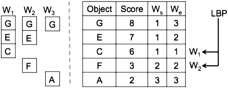
  In order to reach optimal CPU and memory complexity, they propose a single integrated data structure named super-top-k list, for representing all predicted top-k results of future windows. Objects are sorted based on their score in the super-top-k list, and each object has starting and ending window marks which show a set of windows in which the object participate in the top-k result. To efficiently handle new arrival of objects, they define a lower bound pointer ( $\mathit{lbp}$ ) for each window, which points to the object with the smallest score in the top-k list of the window. LBP set contains pointers for all the active windows.

  

  Fig. 3.

  Independent predicted top-k result vs. integrated list of our example in Section 1 at evaluation of the window ${\mathit{w}}_1$ before and after processing changes.

  Considering the example of Fig. 1, where the window length is equal to 9 and each window slides 3 time units, window ${\mathit{W}}_2$ opens at 7 (excluded) and closes at 16, and window ${\mathit{W}}_3$ opens at 10 (excluded) and closes at 19. Assuming that we want to report the top-3 object for each window, the content of super-top-k list at the evaluation of window ${\mathit{W}}_1$ is shown in Fig. 3. During the evaluation of window ${\mathit{W}}_1$ , we have to consider window ${\mathit{W}}_2$ , and ${\mathit{W}}_3$ as future windows.The left side of the picture shows the top-k result for each window. For instance, objects G, E, and C are in the top-3 result of window ${\mathit{W}}_1$ and objects G, E, and F are in the top-3 predicted result of window ${\mathit{W}}_2$ which is started at time 7. The right side shows the super-top-k list which is a compact integrated list of all top-k results. Objects are sorted based on their score. ${\mathit{W}}_{\mathit{s}}$ , and ${\mathit{W}}_{\mathit{e}}$ are window starting and ending marks, respectively. The $\mathit{lbp}$ s of ${\mathit{W}}_1$ , and ${\mathit{W}}_2$ are available, as those windows have top 3 objects in their predicted results.

  The MinTopk algorithm consists of two maintenance steps: handling the expiration of the objects at the end of each window, and handling the insertion of new arrival objects.

  For handling expiration, the top-k result of the expired window must be removed from the super-top-k list. The first k objects in the list with the highest score are the top-k result of the expired window. So, logically purging the first top-k objects of super-top-k list is sufficient for handling expiration. It is implemented by increasing the starting window mark by 1, which means that the object will not be in the top-k list of the expired window anymore. If the starting window mark becomes larger than the end window mark, the object will be removed from the list and the LBP set will be updated if any $\mathit{lbp}$ points to the removed object.

  For insertion of a new object, first the algorithm checks if the new object has the potential to become part of the current or the future top-k results. If all the predicted top-k result lists have k elements, and the score of the new object is smaller than any object in the super-top-k list, the new object will be discarded. If those lists have not reached the size of k yet, or if the score of the new object is larger than any object in the super-top-k list, the new object could be inserted in the super-top-k list based on its score. The starting and ending window marks will also be calculated for the new object. In the next step, for each window, in which the new object is inserted, the object with the lowest score, which is pointed by $\mathit{lbp}$ , will be removed from the predicted top-k result. Like for the purging process, we increase the starting window mark by 1 and if it becomes larger than ending window mark, we physically remove the object from super-top-k list and the LBP set will be updated if any $\mathit{lbp}$ points to the removed object. In order to update $\mathit{lbp}$ pointer, the algorithm simply moves it one position up in the super-top-k list.

  The CPU complexity for MinTopK algorithm is $\mathit{O}\mathrm{(}{\mathit{N}}_{\mathrm{new}}\ast \mathrm{(}log\mathrm{(}\mathit{\text{MTK.size}}\mathrm{)}\mathrm{)}$ in the general case, with $\mathit{O}\mathrm{(}{\mathit{N}}_{\mathrm{new}}\mathrm{)}$ the number of new objects that come in each window, and $\mathit{\text{MTK.size}}$ is the size of super-top-k list. The memory complexity in the general case is equal to $\mathit{O}\mathrm{(}\mathit{\text{MTK.size}}\mathrm{)}$ . In the average case, the size of super-top-k list is equal to $\mathit{O}\mathrm{(}2\mathit{k}\mathrm{)}$ . So, in the average case the CPU complexity is $\mathit{O}\mathrm{(}{\mathit{N}}_{\mathrm{new}}\ast \mathrm{(}log\mathrm{(}\mathit{k}\mathrm{)}\mathrm{)}$ and the memory complexity is $\mathit{O}\mathrm{(}\mathit{k}\mathrm{)}$ . The authors also prove the optimality of the MinTopK algorithms. The experimental studies [40] on real streaming data confirm the out-performance of MinTopK algorithms over the previous solutions.

  Although [40] present an optimal solution for top-k query answering over the data stream, it did not consider join with the distributed dataset, aggregated score, distinct arrival of items, and changes in scoring values. Therefore, MinTopk algorithm does not work properly in such cases.

  3.2. Approximate continuous query answering in RSP engine

  As mentioned in Section 1, RSP engines can join data from streams with distributed data using federated query evaluation, but the time to access and fetch the distributed data can be so high to put the RSP engine at risk of violating the reactiveness requirement.

  The state of the art addressed this problem and offered solutions for RSP engines. S. Dehghanzadeh et al. [10] started investigating Approximate Continuous Query Answering over streams and dynamic Linked datasets (ACQUA). Instead of accessing the whole background data at each evaluation, ACQUA uses a local replica of the background data, and maintenance policies that refresh only a minimum subset of the local replica. Notably [10] considers the class of queries with 1:1 join relationship between the stream and the distributed dataset, as a relevant number of queries in the stream processing context is in this class.

  A maximum number of fetches (namely a refresh budget denoted with γ) at each evaluation guarantees by construction the reactiveness of the RSP engine. If γ fetches are enough to refresh all stale data of the replica, the RSP engine gives the correct answer, otherwise some data items may become stale and it may give an approximated answer.

  The maintenance process introduced in [10] is depicted in Fig. 4, and it is composed of three elements: a proposer, a ranker and a maintainer. The Proposer selects a set of candidates8

  ⁸

  Note that the ACQUA’s candidate set is different from the Minimal Top-k one presented in [40].

  for the maintenance. The Ranker orders the candidate set and the Maintainer refreshes the top γ elements (named elected set). Finally, the join operation is performed after the maintenance of replica.

  

  Fig. 4.

  The framework proposed in [10].

  ACQUA introduces several maintenance policies for updating the local replica. The best performance is obtained combining the proposer (WSJ) and the ranker (WBM). WSJ builds the candidate set by selecting mappings from the replica which are compatible with those in the current window. WBM identifies the mappings that are going to be used in the upcoming evaluations to save future refresh. WBM uses two parameters to order the candidate set by assigning scores defined as: $$\begin{array}{c}{\mathit{score}}_{\mathit{i}}\mathrm{(}\mathit{t}\mathrm{)}=min\mathrm{(}{\mathit{L}}_{\mathit{i}}\mathrm{(}\mathit{t}\mathrm{)}\mathrm{,}{\mathit{V}}_{\mathit{i}}\mathrm{(}\mathit{t}\mathrm{)}\mathrm{)}\mathrm{,}\end{array}$$ where t is the evaluation time, ${\mathit{L}}_{\mathit{i}}\mathrm{(}\mathit{t}\mathrm{)}$ is the remaining life time, i.e. the number of future evaluations that involve the mapping, and ${\mathit{V}}_{\mathit{i}}\mathrm{(}\mathit{t}\mathrm{)}$ is the normalized renewed best before time, i.e., the renewed best before time is normalized with the sliding window parameters.

  Given a sliding window $\mathbb{W}\mathrm{(}\mathit{\omega }\mathrm{,}\mathit{\beta }\mathrm{)}$ , ${\mathit{L}}_{\mathit{i}}$ and ${\mathit{V}}_{\mathit{i}}$ are defined as: $$\begin{array}{ll}\hfill & {\mathit{L}}_{\mathit{i}}\mathrm{(}\mathit{t}\mathrm{)}=\lceil {\displaystyle \frac{{\mathit{t}}_{\mathit{i}}+\mathit{\omega }-\mathit{t}}{\mathit{\beta }}}\rceil \mathrm{,}\\ \hfill & {\mathit{V}}_{\mathit{i}}\mathrm{(}\mathit{t}\mathrm{)}=\lceil {\displaystyle \frac{{\mathit{\tau }}_{\mathit{i}}+{\mathit{I}}_{\mathit{i}}\mathrm{(}\mathit{t}\mathrm{)}-\mathit{t}}{\mathit{\beta }}}\rceil \mathrm{,}\end{array}$$ where ${\mathit{t}}_{\mathit{i}}$ is the time instant associated to the mapping ${\mathit{\mu }}_{\mathit{i}}$ , ${\mathit{\tau }}_{\mathit{i}}$ is the current best before time, and ${\mathit{I}}_{\mathit{i}}\mathrm{(}\mathit{t}\mathrm{)}$ is the change interval that captures the remaining time before the next expiration of ${\mathit{\mu }}_{\mathit{i}}$ . It is worth noting that ${\mathit{I}}_{\mathit{i}}$ is potentially unknown and could require an estimator.

  

  Fig. 5.

  The example that shows how WSJ-WBM policy works.

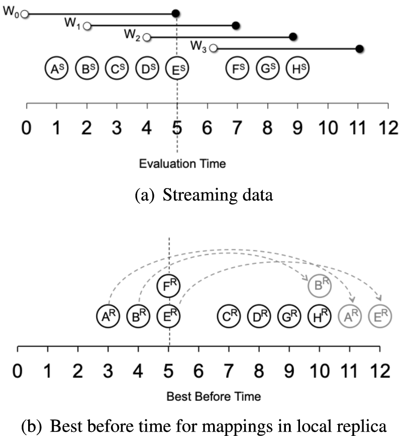
  Figure 5 shows an example that illustrates how WSJ-WBM policy works. Figure 5(a) shows the mappings that enter the window clause between time 0 and 12. Each window has a length of 5 units of time and slides every 2 units of time. For instance, window ${\mathit{W}}_0$ opens at 1 (excluded) and closes at 6. Each mapping is marked with a point and for the sake of clarity, we label each point with ${\mathit{I}}^{\mathit{S}}$ where I is the ID of the subject of mapping and S indicates that the mappings appear on the data stream. So, for example during window ${\mathit{W}}_0$ mappings ${\mathit{A}}^{\mathit{S}}$ , ${\mathit{B}}^{\mathit{S}}$ , ${\mathit{C}}^{\mathit{S}}$ , ${\mathit{D}}^{\mathit{S}}$ , and ${\mathit{E}}^{\mathit{S}}$ appear on the data stream.

  Figure 5(b) shows the mappings in the local replica. The mappings in the replica are indicated by R. The replica contains mappings ${\mathit{A}}^{\mathit{R}}\mathrm{,}{\mathit{B}}^{\mathit{R}}\mathrm{,}\dots \mathrm{,}{\mathit{H}}^{\mathit{R}}$ . The X axis shows the value of best before time for each mapping. It is worth to note that points with the same ID in Figs 5(a), and 5(b) indicates compatible mappings.

  At the end of window ${\mathit{W}}_0$ , at time 5, WSJ computes the candidate set by selecting compatible mappings with the ones in the window. The candidate set C contains mappings ${\mathit{A}}^{\mathit{R}}$ , ${\mathit{B}}^{\mathit{R}}$ , ${\mathit{C}}^{\mathit{R}}$ , ${\mathit{D}}^{\mathit{R}}$ , and ${\mathit{E}}^{\mathit{R}}$ . ${\mathit{F}}^{\mathit{R}}$ , ${\mathit{G}}^{\mathit{R}}$ , and ${\mathit{H}}^{\mathit{R}}$ are excluded from C because they are not compatible. In the next step, WSJ-WBM finds the possible stale mappings by comparing their best before time values with the current time. The possibly stale mappings are $\mathit{PS}=\{{\mathit{A}}^{\mathit{R}}\mathrm{,}{\mathit{B}}^{\mathit{R}}\mathrm{,}{\mathit{E}}^{\mathit{R}}\}$ . The best before time of other mappings are greater than the current time, so they do not need to be refreshed.

  The remaining life time shows the number of successive evaluations for each mapping. The remaining life time of mapping ${\mathit{A}}^{\mathit{R}}$ , ${\mathit{B}}^{\mathit{R}}$ , ${\mathit{E}}^{\mathit{R}}$ are 1, 1 and 3, respectively. Figure 5(b) shows the renewed best before time of the elements in $\mathit{PS}$ by the dashed light gray arrows. The renewed best before time ( ${\mathit{\tau }}_{\mathit{i}}+{\mathit{I}}_{\mathit{i}}\mathrm{(}\mathit{t}\mathrm{)}-\mathit{t}$ ) of mappings ${\mathit{A}}^{\mathit{R}}$ , ${\mathit{B}}^{\mathit{R}}$ , ${\mathit{E}}^{\mathit{R}}$ are respectively 11, 10, and 12. Therefore, considering $\mathit{t}=5$ , and $\mathit{\beta }=2$ , the normalized renewed best before time ( ${\mathit{V}}_{\mathit{i}}\mathrm{(}\mathit{t}\mathrm{)}$ ) of mappings ${\mathit{A}}^{\mathit{R}}$ , ${\mathit{B}}^{\mathit{R}}$ , ${\mathit{E}}^{\mathit{R}}$ at time 5 are respectively 3, 3 and 4. Finally, the score will be computed for each mapping at time 5: ${\mathit{score}}_{\mathit{A}}\mathrm{(}5\mathrm{)}=1$ , ${\mathit{score}}_{\mathit{B}}\mathrm{(}5\mathrm{)}=1$ , and ${\mathit{score}}_{\mathit{E}}\mathrm{(}5\mathrm{)}=3$ . Given the refresh budget γ equal to 1, the elected mapping will be ${\mathit{E}}^{\mathit{R}}$ , which has the highest score.

  Other rankers proposed in [10] are (i) LRU that, inspired by the Least-Recently Used cache replacement algorithm, orders the candidate set by the time of the last refresh of the mappings (the less recently a mapping has been refreshed in a query, the higher is its rank), and (ii) RND that randomly ranks the mappings in the candidate set.

  As already stated in the introduction, ACQUA is not optimal for top-k queries. Intuitively, WSJ-WBM policy may update mappings that do not contribute to the top-k result and can sub-optimally utilize the available refresh budget. In the next section, we elaborate on an extension that, instead, focuses on the top-k results.

  4. Topk+N solution

  In this section, we introduce the proposed solution to the problem of the top-k approximate join of streaming and evolving distributed data in the context of RSP engines. As we repeated multiple times, being reactive is the most important requirement, while we have changes in the distributed dataset. Section 4.1 shows how we extend the approach in [40] for joining streaming and evolving distributed data. Section 4.2 introduces the MTK+N data structure. In Section 4.3, we define the Super-MTK+N list. Finally, in Section 4.4, we explain the Topk+N algorithm, which is optimized for the top-k approximate join.

  4.1. MinTopk+

  As mentioned in Section 3.1, MinTopk [40] offers an optimal strategy to monitor top-k query evaluation over streaming data. In this section, we report on how to extend MinTopk to handle changes in the distributed dataset.

  Let us assume that the distributed dataset notifies changes to the engine that has to answer the query. First of all, it is important to note that MinTopk assumes distinct arrivals, so, it cannot be applied if the changed object has been already processed in the current window. The first contribution of this paper is, therefore, an extension of MinTopk algorithm to consider indistinct arrival of objects. We name this algorithm MinTopk $\mathbf{+}$ .

  If the changed object exists in the super-top-k list, we removed the old object from the super-top-k list, and we add the object with the new score to the super-top-k list. If the changed object is not in the list of top-k predicted results, we have to consider it as a new arrival object and check if, with the new score, it could be inserted in the top-k list. This second case is not feasible in practice, as it requires to store the value of the scoring variable ${\mathit{x}}_{\mathcal{S}}$ for all the streaming data that entered the current window, while the goal of MinTopk is to discard all streaming data that does not fit in the predicted top-k results of the active windows.

  As a work around, we propose: (1) to keep the minimum value of the scoring variable ${\mathit{x}}_{\mathcal{S}}$ that has been seen while processing the current window. Let us denote it as $\mathit{\text{min}}.{\mathit{\text{score}}}_{\mathcal{S}}$ . (2) to generate an approximated score for the changed object using $\mathit{\text{min}}.{\mathit{\text{score}}}_{\mathcal{S}}$ as the streaming score of the changed object. As the scoring variable ${\mathit{x}}_{\mathcal{S}}$ of the changed object cannot be lower than $\mathit{\text{min}}.{\mathit{\text{score}}}_{\mathcal{S}}$ , the generated new score is a lower bound for the real new score.

  As we don’t need to keep the scoring variable of all arrival objects in the current window, MinTopk+ (as MinTopk) is not depended on the size of the data in the window, and a subset of data is enough for top-k approximated join. We further elaborate on this idea in Sections 4.4 and 5.3 where we, respectively, formalize how the $\mathit{\text{min}}.{\mathit{\text{score}}}_{\mathcal{S}}$ is computed and where we study the memory and time complexity of a generalized version of this algorithm.

  4.2. Updating minimal Top-K+N candidate list

  Considering the changes in the distributed dataset, which affect the top-k result, in this section, we propose an approach that gives the correct answer in the current window in most of the cases and, in some cases, may give an approximated answer.

  The authors in [40] proposed MTK set which is necessary and sufficient for evaluating continuous top-k query. We extend the MTK set by considering changes of the objects and keeping N additional objects, and introduce Minimal Top-K $\mathbf{+}$ N Candidate list (MTK $\mathbf{+}$ N list). MTK+N list keeps K+N ordered objects that are necessary to generate top-k result. The following analysis shows that MTK+N list is also sufficient for generating the correct result in the current window for most of the cases.

  Assume that we have N changes per evaluation in the distributed dataset, and we keep K+N objects for each window in the predicted result. Each MTK+N list consists of two areas. Let us name them K-list and N-list. Therefore, each object can be placed in 3 different areas: K-list, N-list, and outside (i.e. outside the MTK+N list). For example, assuming k is equal to 2, and N is equal to 1, in Fig. 3, the MTK+N list of window ${\mathit{W}}_1$ contains objects G, and E in the k-list, and object C in the N-list.

  It is worth to note that each object can be placed in different areas in different MTK+N lists. The position of the object can change between those areas due to changes to the values assumed by the scoring variables ${\mathit{x}}_{\mathcal{D}}$ in the distributed dataset. Depending on the initial and the destination areas of each object, we may have exact or approximated result in each window. The following theorems analyze different scenarios for each window separately, and assuming that (i) the previous results are correct,9

  ⁹

  The approximated results in previous evaluations lead to approximated result in the current window.

  (ii) we have N changes per evaluation in the distributed dataset, and (iii) we keep K+N objects for each window in the predicted result.

  Theorem 1.

  If the changed object is in the K-list, or the N-list and remains in one of them, or if the changed object is initially outside of the MTK + N list and remains outside, we can report the correct top-k result for the corresponding window (current, or future).

  Proof.

  If the changed object exists in the MTK+N list, we have got the previous score of the object. The new score can only change the place of the object in the list. If the changed object is outside of the list and remains outside, we do not modify the MTK+N list. In both cases, we have the correct result.  □

  Theorem 2.

  If the changed object was in the K-list, or the N-list, and the new score removes it from MTK + N list, we can report the correct top-k result for the corresponding window.

  Proof.

  If the changed object o exists in the MTK+N list, but the new score is less than the lowest score in the MTK+N list, we have to remove the object from MTK+N list. As all the objects in the K-list are placed correctly, we have the exact result for the current window. However, after removing it, we have one empty position in MTK+N list. If we do not have any other objects in the MTK+N lists of future windows, which fit into the current MTK+N list, we can only add o back with the new score. In previous evaluations, we may have another object with higher score comparing to the new one of o, but it did not satisfy the constraints to be in the MTK+N list at that point in time, and we discarded it. When that happens, the forgotten object is misplaced by object o. If during the evaluation of the window, the misplaced object o comes up in the K-list, we do not have the correct result.  □

  Theorem 3.

  If the changed object initially is outside the MTK + N list, and, after the changes, it moves in the MTK + N list, we may have approximated result for the corresponding window.

  Proof.

  When the changed object o is not in the MTK+N list, we cannot access to the previous information of the object in the data stream, we do not know if it appeared in the streaming data or not, and if yes, what was the value of scoring variable ${\mathit{x}}_{\mathcal{S}}$ . To solve this problem two different approaches can be considered: first, we can just ignore the changed objects o which are not in the MTK+N list, second, we can keep pointers to the objects come in the streaming data in each window and also keep the minimum score of them as $\mathit{\text{min}}.{\mathit{\text{score}}}_{\mathcal{S}}$ .

  Table 1

  Summary of scenarios in handling changes

  		Initial Area
  		K-list	N-list	Outside
  Destination Area	K-list	V	V	${\mathit{V}}^{\mathit{precision}@\mathit{k}}$ , ${\approx }^{\mathit{nDCG}@\mathit{k}}$
  	N-list	V	V	≈
  	Outside	V, ≈	V, ≈	V

  Focusing on the second approach, we are able to generate an approximated score for o. The new approximated score of object o can be generated using $\mathit{F}\mathrm{(}\mathit{\text{min}}.{\mathit{\text{score}}}_{\mathcal{S}}\mathrm{,}\mathit{o}.{\mathit{\text{score}}}_{\mathcal{D}}\mathrm{)}$ and the changed value of scoring variable in the distributed dataset, which is the minimum threshold for the real score. The changed object may fit in different areas:

  If it moves in the K-list, as the new score is a minimum threshold for real score, the real score of the object will also put it in the K-list. However, being the approximated score a lower bound, the real score may position it in a higher ranked place. So, considering $\mathit{precision}@\mathit{k}$ , we have the exact result, while considering $\mathit{nDCG}@\mathit{k}$ , we may have an approximated result.

  If it moves in the N-list, as the new score is a minimum threshold, the real score of the object may put it in the K-list, so we have approximated result for the window.  □

  Table 1 summarizes all the explained scenarios. Assuming that we have exact result up to current time, each cell shows the correctness of the top-k result as a function of the initial and destination areas of the changed object. The exact result is indicated by V, while the approximation in the result is showed by ≈. $\mathit{precision}@\mathit{k}$ and $\mathit{nDCG}@\mathit{k}$ shows the metrics used for comparing the real result with the correct one.

  Theoretically, introducing another area, between N and the outside areas, can increase the correctness of the result and avoid approximation for the upcoming future windows. Considering the size of this new area equal to N, the result of the next window will also be correct for all scenarios. But, practically, the result of the experiments in Section 6 shows that keeping K+N objects in MTK+N list is often enough.

  4.3. Super-MTK+N list

  When a query expressed on a sliding window, the predicted top-k results of the current and future windows have partial overlaps. So we have objects which are repeated in the MTK+N lists of the current and future windows. In order to minimize the memory usage, a single integrated list for all active windows can be used instead of various MTK+N lists.

  Therefore, we define the Super-MTK $\mathbf{+}$ N list that consists of several MTK+N lists of all active window (current and future). The objects in Super-MTK+N list are ordered based on their scores. In order to distinguish the top-k result of each window, for each object we define starting and ending window marks. The marks of each object show the period in which it is in the predicted top-k result.

  Table 2

  List of symbols used in the algorithms

  Symbol	Description
  MTK+N	Minimal Top-K+N list of objects
  Super-MTK+N	Compact representation for MTK+N lists of objects for all active windows
  ${\mathit{O}}_{\mathit{i}}$	An arriving object
  ${\mathit{O}}_{\mathit{i}}.\mathit{t}$	Arriving time of object ${\mathit{O}}_{\mathit{i}}$
  ${\mathit{O}}_{\mathit{i}}.\mathit{w}.\mathit{\text{start}}$	Starting window mark of ${\mathit{O}}_{\mathit{i}}$
  ${\mathit{O}}_{\mathit{i}}.\mathit{w}.\mathit{\text{end}}$	Ending window mark of ${\mathit{O}}_{\mathit{i}}$
  ${\mathit{O}}_{\mathit{i}}.\mathit{\text{score}}$	Score of object ${\mathit{O}}_{\mathit{i}}$
  ${\mathit{w}}_{\mathit{i}}.\mathit{l}\mathit{b}\mathit{p}$	The lower bound pointer of ${\mathit{w}}_{\mathit{i}}$ which points to the object with smallest score in the window ${\mathit{w}}_{\mathit{i}}$
  $\mathit{LBP}$	Set of lower bound pointers for all windows that have top k objects in Super-MTK+N list
  ${\mathit{O}}_{{\mathit{w}}_{\mathit{i}}.\mathit{\text{lbp}}}$	Object pointed by ${\mathit{w}}_{\mathit{i}}.\mathit{l}\mathit{b}\mathit{p}$
  ${\mathit{w}}_{\mathit{i}}.\mathit{\text{tkc}}$	The number of items in top-k result of window ${\mathit{w}}_{\mathit{i}}$
  ${\mathit{W}}_{\mathrm{act}}$	List of active windows which contain current time in their duration
  ${\mathit{O}}_{\mathrm{minScore}}$	The object with smallest score in the Super-MTK+N list
  $\mathit{MTK}+\mathit{N}.\mathit{\text{size}}$	Size of MTK+N list which is equal to K+N
  ${\mathit{w}}_{max}$	Maximum number of windows
  ${\mathit{w}}_{exp}$	The window just expired
  $\mathit{\text{min}}.{\mathit{\text{score}}}_{\mathcal{S}}$	Minimum value of scoring variable ${\mathit{x}}_{\mathcal{S}}$ seen on the data stream while processing the current window

  4.4. Topk+N algorithm

  As mentioned in the previous section, we extend the integrated data structure MTK list from [40] and introduce Super-MTK+N list to handle changes in the distributed dataset. In this section, we describe the Topk $\mathbf{+}$ N algorithm that evaluates top-k queries over streaming and evolving distributed data. Table 2 contains the description of symbols used in Algorithms 1, 2, 3, 4, and 5.

  The evaluation of a continuous top-k query over a sliding window needs to handle the arrival of new objects in the stream and removal of old objects in the expired window. In addition to the state-of-the-art approach [40], in this problem setting we have changes in the distributed dataset. So, we have to also handle those changes during query processing. The proposed algorithm consists of three main steps: expiration handling, insertion handling, and change handling.

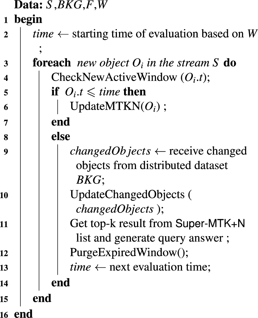
  Algorithm 1 shows the pseudo-code of Topk+N algorithm which gets in input the data stream S, the distributed data $\mathit{BKG}$ , the scoring function F, and the window W and generates the top-k result for each window. In the beginning, the evaluation time is initialized. For every new arrival object ${\mathit{O}}_{\mathit{i}}$ , in the first step, it checks if any new window has to be added to the active window list (Line 4). The algorithm keeps all the active windows in a list named ${\mathit{W}}_{\mathrm{act}}$ . In the next step, it checks if the time of arrival is less than the next evaluation time (i.e., the ending time of the current window), and it updates the Super-MTK+N list if the condition is satisfied (Lines 5–7).

  Otherwise, at the end of the current window, it checks for the received changes from the distributed dataset (Line 9). Function UpdateChangedObjects (Line 10) gets the set changedObjects and updates Super-MTK+N list based on changes. This function is the main contribution of the Topk+N Algorithm comparing to the MinTopk algorithm [40]. Getting the top-k result from Super-MTK+N list, the algorithm generates the query result (Line 11). Finally, it purges the expired window and goes to the next window processing (Lines 12–13).

  
  Algorithm 1:

  The pseudo-code of Topk+N algorithm

  4.4.1. Expiration handling

  When a window expires, we have to remove the corresponding top-k result from the Super-MTK+N list. We cannot simply remove the objects, as we have integrated view of the top-k results in Super-MTK+N list, and some of the top-k objects may be also in the top-k results of the future windows. We can implement removing of these object from the list by updating their window marks and increasing the starting window marks by 1 for all the objects in the top-k result of the expired window.

  Function PurgeExpiredWindow (Line 1) in Algorithm 2 shows the pseudo-code of expiration handling. It gets the first top-k objects from Super-MTK+N list, whose starting window mark is equal to the expired window and increases their starting window mark by 1 (Line 5). If the starting window mark becomes larger than the end window mark, the object is removed from Super-MTK+N list. The LBP set is updated if any pointer to the deleted object exists (Lines 8–11). Finally, the expired window is removed from the Active Windows list and LBP set (Lines 16–17), and the value of $\mathit{\text{min}}.{\mathit{\text{score}}}_{\mathcal{S}}$ is reset (Lines 18).

  
  Algorithm 2:

  The pseudo-code of expiration handling

  
  Fig. 6.

  Super-MTK+N list content related to the example of Section 1 in different evaluation times.

  Consider the example of Fig. 1, where window ${\mathit{W}}_0$ opens at 1 (excluded) and closes at 10. Assume that we are at time 10, when window ${\mathit{W}}_0$ is expired, and we want to report the top-3 objects as result. Figure 6(a) shows the content of Super-MTK+N list. For window expiration, the starting window marks of the objects E, C, and B have to be increased by 1. Object B is removed from the list, as its starting window mark becomes larger than the end window mark. The $\mathit{lbp}$ s of ${\mathit{W}}_0$ is also removed from the LBP set. Figure 6(b) shows the Super-MTK+N list after expiration handling of window ${\mathit{W}}_0$ .

  4.4.2. Handling new arrivals and changes

  When a new object arrives in the stream, we have to check if it can be added to the top-k result of current and future windows or not, so its score should be compared with the minimum score in the Super-MTK+N list and if all the predefined conditions are satisfied we can insert it to the Super-MTK+N list. We treat the changed object as a new arrival object and we check if it can be added to the Super-MTK+N list. If the changed object exists in the Super-MTK+N list, it should be replaced with the old one.

  Topk+N algorithm (see Algorithm 3 for the pseudo-code) updates Super-MTK+N list based on new arriving objects on the stream S. For every object ${\mathit{O}}_{\mathit{i}}$ in the stream, function UpdateMTKN checks if the object ${\mathit{O}}_{\mathit{i}}$ can be inserted in the Super-MTK+N list or not. At the first step, if the streaming score of the object is less than the value of $\mathit{\text{min}}.{\mathit{\text{score}}}_{\mathcal{S}}$ , the minimum score should be updated (Lines 2–4). Keeping the minimum score let us approximate the score for changed objects as discussed in Section 4.1. Then, it checks if the object ${\mathit{O}}_{\mathit{i}}$ is present in the Super-MTK+N list, since Topk+N algorithm supports indistinct arrivals (different from state of the art [40]). If the Super-MTK+N list contains a stale version of ${\mathit{O}}_{\mathit{i}}$ , it is replaced with the fresh one. As the score of the replaced object ${\mathit{O}}_{\mathit{i}}$ changed, its position in Super-MTK+N list can change too and it may move up or down in the list. Changing position in the Super-MTK+N list could affect the top-k results of some of the active windows, thus the LBP set needs to be refreshed. Otherwise, when the object is not present in the Super-MTK+N list, the algorithm (1) computes the score, the starting window mark, and the ending window marks; (2) it inserts the object in the Super-MTK+N list; and (3) updates the LBP set.

  
  Algorithm 3:

  The pseudo-code for updating Super-MTK+N list

  Algorithm 3 shows in more details the pseudo-code for handling insertion of new arriving objects through the update of the Super-MTK+N list. If a stale version of the arriving object exists in Super-MTK+N list, the algorithm replaces it with the fresh one with new values i.e., its score, and its starting/ending window marks (Line 6). Then, we have to refresh the LBP set based on the changes occurred in Super-MTK+N list (Line 7). As the new values of the arriving object could change the order of objects in the Super-MTK+N list, the LBP set is recomputed. In case the object is not in the Super-MTK+N list, it computes the score, and adds the new object in the list (Line 16). If the object is a new arrival, computing the score from the values of the scoring variables is straightforward, but if object ${\mathit{O}}_{\mathit{i}}$ is a changed object, the new score is computed getting the value of $\mathit{\text{min}}.{\mathit{\text{score}}}_{\mathcal{S}}$ and the scoring value in the replica (Line 11), as we did not keep the scoring value of all the objects, but only of those that entered the Super-MTK+N list (see also Section 4.1, where we present this idea).

  Function InsertInToMTKN handles object insertion to the Super-MTK+N list. If the score of the object ${\mathit{O}}_{\mathit{i}}$ is smaller than the minimum score in the Super-MTK+N list, and all active windows contain k objects as top-k result, then the arriving object is discarded (Lines 19–21). Otherwise, the future windows, in which the object can be in the top-k result, are defined by computing the starting and the ending window marks (Lines 23–24). In the next step, the object is inserted into the Super-MTK+N list and the LBP set is updated (Line 26).

  Function UpdateChangedObjects is used for updating Super-MTK+N list for a set of objects, and gets the Objects set as input. For each object in the Objects set, it updates the Super-MTK+N list by refreshing the stale object in the Super-MTK+N list (Line 31).

  4.4.3. Updating lower bound pointers

  As mentioned in Section 3.1, LBP is a set of pointers to the top-k objects with the smallest scores for all active windows that have k objects as top-k result. When a new object arrives, we need to compare its score with those of the objects pointed by LBP for each window. If the size of any predicted top-k result for future windows is less than the size of MTK+N list (i.e. K+N), or the new object has a higher score comparing to the objects that have $\mathit{lbp}$ s, the new object can be inserted in the Super-MTK+N list.

  After inserting the new object, the LBP set needs to be updated; in particular, those pointers that relate to the windows between the starting and the ending window marks of the inserted object. For those windows that have not got any pointer in the LBP set, the size of the top-k result is increased by 1. If the size becomes equal to k, the pointer is created for the window and added to the LBP set.

  
  Algorithm 4:

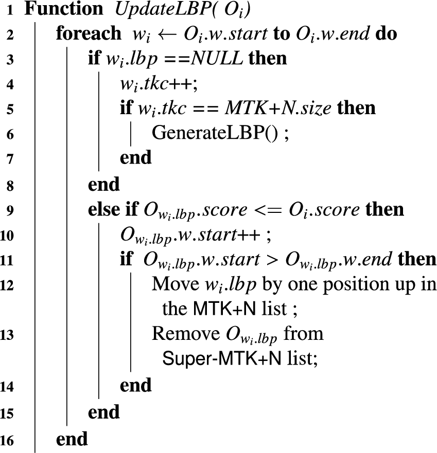
  The pseudo-code for updating LBP list

  If the window has got a pointer in LBP set and the score of the inserted object is less than the score of the pointed object, then the last top-k object in the predicted result is removed from the list, so we have to increment the starting window mark by 1. If the starting window mark becomes greater than the ending window mark for any object, the pointer moves up by one position in the Super-MTK+N list and the object is removed from Super-MTK+N list.

  Algorithm 4 shows the pseudo-code for updating the LBP set after inserting the new object to the Super-MTK+N list. For all the affected windows from the starting to the ending window marks of the inserted object, if the window does not have any $\mathit{lbp}$ , we increment the cardinality of top-k result by 1 (Line 4). If the cardinality of top-k result of a window reaches the K+N, Function GenerateLBP generates the pointer to the last top-k object of that window and adds it to the LBP set (Line 6).

  If the window has a pointer in LBP set, we compare the score of the inserted object with the score of the pointed object (i.e. the last object in top-k result with lowest score). If the inserted object has higher score, we remove the last object in top-k result by increasing the starting window mark by 1 (Line 10). If the starting window mark of the object becomes greater than ending window mark, we move the lbp one position up in the Super-MTK+N list and remove the object from Super-MTK+N list (Lines 11–14).

  Let us consider our example in Fig. 1 at time 11. Figure 6(b) shows the content of Super-MTK+N list after the expiration of window ${\mathit{W}}_0$ . At time 11, object A comes to the system, and based on its score it is inserted to the Super-MTK+N list with starting window mark equal to 2 and ending window mark equal to 3. As now we have 3 objects in window ${\mathit{W}}_2$ , the $\mathit{lbp}$ of the window is added to the LBP set. Figure 6(b) shows the changes applied on the Super-MTK+N list.

  At time 12, object G comes to the system, and inserted at the top of the Super-MTK+N list. As Windows ${\mathit{W}}_1$ , and ${\mathit{W}}_2$ have 3 objects in their top-3 result, we have to remove the last object of each window. So the starting window marks of objects C and F need to be increased by one, and $\mathit{lbp}$ of Windows ${\mathit{W}}_1$ , and ${\mathit{W}}_2$ should be modified. Object F was the last object in the result of window ${\mathit{W}}_1$ , and after inserting object G, object C becomes the last object and $\mathit{lbp}$ of Windows ${\mathit{W}}_1$ points to it. For window ${\mathit{W}}_2$ , the last object changes from object A to object F, and the $\mathit{lbp}$ moves one position up accordingly.

  
  Fig. 7.

  Independent predicted top-k result vs. integrated list of our example in Section 1 at evaluation of window ${\mathit{w}}_1$ after processing changes.

  
  Fig. 8.

  The AcquaTop framework.

  Figure 7 shows how handling changes could affect the content of the Super-MTK+N list and of the top-k query result. At the evaluation time of ${\mathit{W}}_1$ , after handling new arrivals of window ${\mathit{W}}_1$ , the content of the Super-MTK+N list is as in Fig. 3. As the score of object E changes from 7 to 10 (Fig. 1(c)), it is considered as an arriving object with a new score, so, it is placed in the Super-MTK+N list above object G. The LBP set does not change in this case. As we mentioned in Section 4.2, each object can be placed in different areas in different MTK+N lists. For example, in Fig. 7, assuming K = 1, and N = 2, object G is in the N-list of windows ${\mathit{W}}_1$ , and ${\mathit{W}}_2$ , but it is placed in the k-list of window ${\mathit{W}}_3$ .

  Comparing to the MinTopk algorithm [40], the Topk+N algorithm has the following additional futures: (i) it computes the minimum score on the streaming side to approximate score of changed objects, (ii) it handles distinctive arrival of objects, and (iii) it handles changed objects.

  5. AcquaTop solution

  Using Super-MTK+N list and Topk+N algorithm, we are able to process continuous top-k query over streaming and distributed data while getting notification of changes from the distributed dataset. As we anticipated in Section 1, this solution works in a data center, where the entire infrastructure is under control, but it does not when we may have high latency, low bandwidth and even rate-limited access as in the two examples of Section 1. In those cases the engine, which continuously evaluates the query, has to pull the changes from the distributed dataset and, thus, the reactiveness requirement can be violated.

  In this section, we present AcquaTop solution to address this problem. Section 5.1 introduces the AcquaTop Framework. In Section 5.2, we present the details of the AcquaTop algorithm, and two new maintenance policies. Finally, Section 5.3 presents a cost analysis of AcquaTop algorithm.

  5.1. AcquaTop framework

  As mentioned in Section 3.2, ACQUA [10] addresses this problem by keeping a local replica of the distributed data and using several maintenance policies to refresh such a replica. Considering the architectural approach presented in [10] as a guideline, we propose a second solution to our problem, named AcquaTop framework. It keeps a local replica of the distributed data and updates the part of it that affects the most the current and future top-k answer after every evaluation.

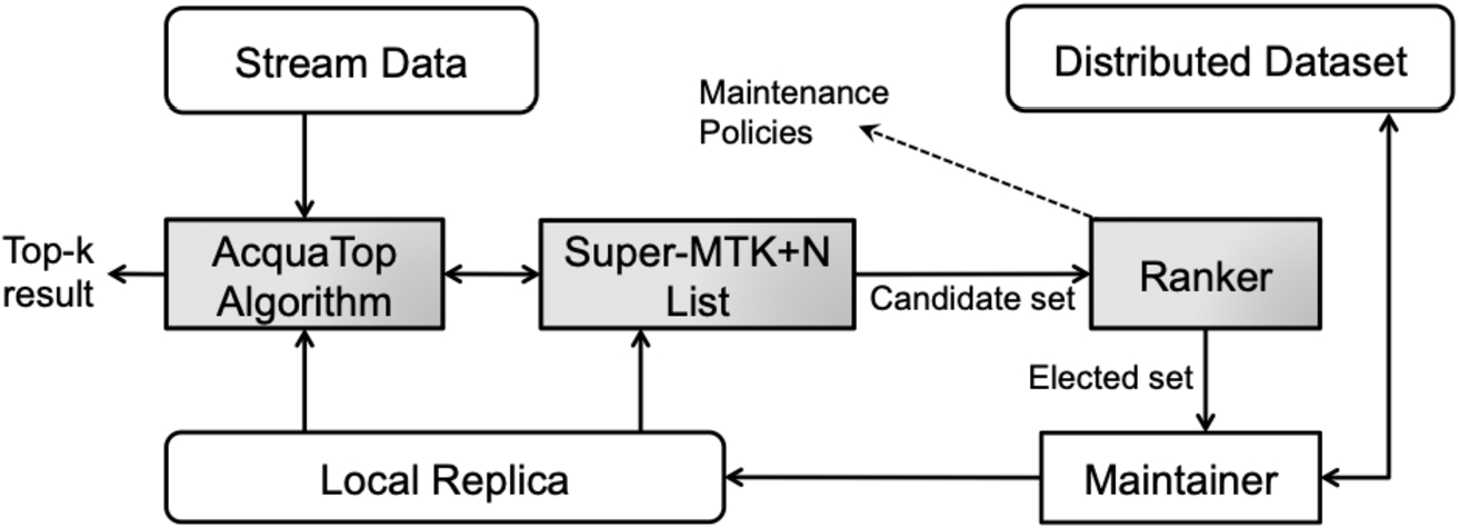
  Figure 8 shows the architecture of AcquaTop framework. AcquaTop gets data from the stream and the local replica and, using Super-MTK+N list structure, it evaluates continuous top-k query at the end of each window. The Super-MTK+N list provides the Candidate set for updating. Notably, such a set is a small subset of the objects that logically should be stored in the window since our approach discards objects that do not enter in the predicted top-k results when they arrive. The Ranker gets the Candidate set and orders them based on the criteria of the different maintenance policies. The maintainer get the top γ elements, namely the Elected set, where γ is the refresh budget for updating the local replica.

  When the refresh budget is not enough to update all the stale elements in the replica, we might have some errors in the result. Therefore, as in ACQUA, we propose different maintenance policies for updating the replica, in order to approximate as much as possible the correct result. In the following, we introduce AcquaTop algorithm and the proposed maintenance policies.

  
  Algorithm 5:

  The pseudo-code of AcquaTop algorithm

  5.2. AcquaTop algorithm

  In top-k query evaluation, after processing the new arrivals of each window, we prepare the set of objects which have been updated in the local replica by fetching a fresher version from the distributed dataset. Algorithm 5 shows the pseudo-code of AcquaTop Algorithm for handling changes in the local replica in addition to handling insertion of new arrival objects.

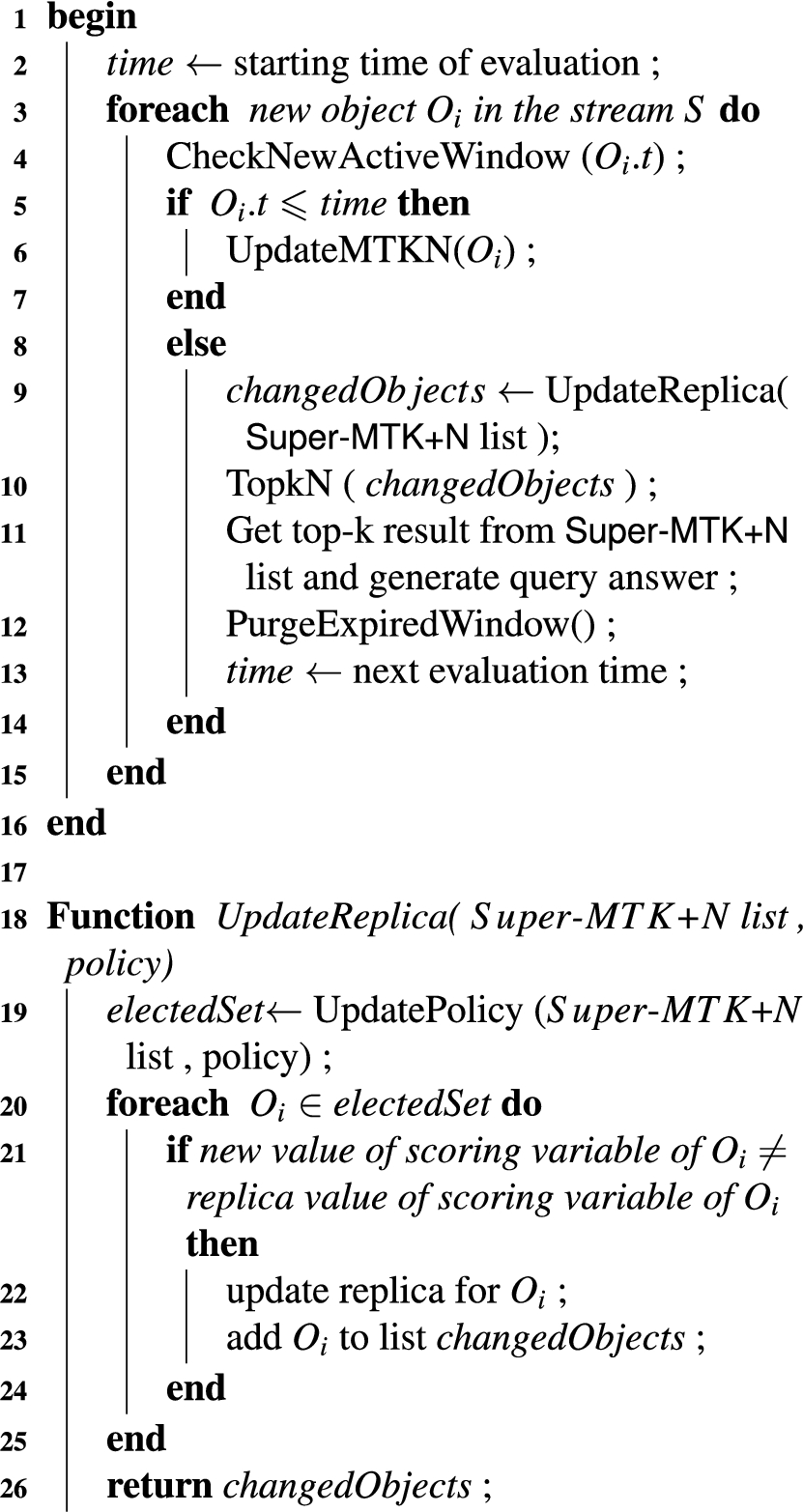
  In the first step, the evaluation time is initialized. Then, for every new arriving objects, it checks if any new window has to be added to the active window list (Line 4). If the time of arrival is less than the next evaluation time (i.e., the ending time of the current window), it updates the Super-MTK+N list (Lines 5–7).

  At the end of the current window, Function UpdateReplica gets the Super-MTK+N list and returns the set of changed objects in the replica (Line 9). Then, Function TopkN (Line 10) gets the set changedObjects and updates Super-MTK+N list based on changes. The algorithm considers changed objects as new arriving objects with different scores. It removes the stale version of the object from the Super-MTK+N list and reinserts it if the constraints are satisfied. Then, getting the top-k result from Super-MTK+N list, the algorithm returns the query answer (Line 11). Finally, it purges the expired window and goes to the next window processing (Lines 12–13).

  Function UpdateReplica in Algorithm 5 updates the replica getting the Super-MTK+N list and the $\mathit{policy}$ as inputs. Function UpdatePolicy (Line 19) gets the Super-MTK+N list and the $\mathit{policy}$ . Then based on different maintenance policies, it returns the electedSet of objects for updating. For every object in the electedSet, if the new value of the scoring variable ${\mathit{x}}_{\mathcal{D}}$ and the one in replica are not the same, it updates the replica and puts the object in the set changedObjects (Lines 20–25). Finally, Function UpdateReplica returns the set changedObjects.

  In the following sections, we propose different maintenance policies. Function UpdatePolicy gets one of them as input and generates the electedSet of objects for updating the local replica. The following four sections detail our maintenance policies.

  5.2.1. Top selection maintenance policy (AT-TSM)

  Maintenance policies specific for top-k query evaluation are the key contributions of this paper. The intuition for these policies is straightforward: since AcquaTop algorithm makes it possible to predict the top-k result of the future windows, updating the replica for those predicted objects catches the opportunity to generate more accurate results. As a consequence, the rest of the data in the replica has less priority for updating.

  The predicted top-k results of future windows are kept in the Super-MTK+N list. Based on AcquaTop algorithm, as we have got a sliding window, the top-k objects of the current window have high probabilities to be in the top-k result of future windows. Therefore, updating the top-k objects can affect the relevance of the result of future windows more than updating objects far from the first top-k. Based on this intuition, The Top Selection Maintenance (AT-TSM) policy selects objects from the top of the Super-MTK+N list for updating the local replica. The proposed policy gives priority to the object with higher rank, as it focuses on more relevant result. Our hypothesis is that comparing to the other policies, AT-TSM can have higher value of $\mathit{nDCG}@\mathit{k}$ .

  For Example, let us assume that k is equal to 3, N is equal to 1, and γ is equal to 2, considering the example introduced in Section 1, and the Super-MTK+N list showed in Fig. 6(d), at the end of window ${\mathit{W}}_1$ , AT-TSM policy selects object G and E for updating from the top of the Super-MTK+N list.

  5.2.2. Border selection maintenance policy (AT-BSM)

  Super-MTK+N list contains K+N objects for each window, and each object in the predicted result is placed in one of the following areas: the K-list, which contains the top-k objects with the highest rank; or the N-list, which contains the next N items after top-k ones. The Border Selection Maintenance (AT-BSM) policy focuses on the objects around the border of those two lists and selects objects for updating around the border.

  The intuition behind AT-BSM is that objects around the border have higher chances to move between the K- and the N-list [42]. Indeed, updating those objects may affect the top-k result of future window. The policy concentrates on the objects that may be inserted in or removed from top-k result and can generate more accurate results. So, our hypothesis is that comparing with other policies, AT-BSM policy has higher value of $\mathit{precision}@\mathit{k}$ .

  For example, considering Fig. 6(d), and assuming that k is equal to 3, N is equal to 1, and γ is equal to 2, AT-BSM policy selects objects C and F for updating from the border of the K- and the N-list in the Super-MTK+N list.

  5.2.3. All selection maintenance policy (AT-ASM)

  The upper bound accuracy and relevancy of AcquaTop is the case when there is no limit for the refresh budget, i.e. we can update all the elements in the Super-MTK+N list. We name this policy All Selection Maintenance (AT-ASM) policy. Our hypothesis is that AT-ASM policy has the maximum accuracy and relevancy as it has no constraint on the number of accesses to the distributed dataset, and updates all the objects in the predicted top-k results. The only reason why it approximates result are the cases presented in Table 1 referring to Theorems 1, 2, and 3. However, AT-ASM policy is not a feasible solution in practice, as it does not consider the limitation on the number of accesses to the distributed dataset, and can put the system at the risk of losing reactiveness. We only use AT-ASM policy to verify the correctness of the experiments reported in Section 6. In our example of Fig. 6(d), AT-ASM policy updates all the objects in the Super-MTK+N list.

  5.2.4. AT-LRU and AT-WBM policies

  As an alternative to previous three policies, we can use AcquaTop algorithm and Super-MTK+N list to evaluate the top-k query, while applying state-of-the-art maintenance policies from ACQUA [10] for updating the local replica. ACQUA shows that WSJ-WBM and WSJ-LRU policies perform better than others while processing join query. We combine those policies with AcquaTop algorithm and propose the following policies: AT-LRU, and AT-WBM. Our hypothesis is that AT-LRU works when most recently used objects appear in the top-k result of future windows. AT-WBM policy works when we have a correlation between being in the top-k result and staying longer in the sliding window.

  5.3. Cost analysis

  The memory size required for each object ${\mathit{o}}_{\mathit{i}}$ in the Super-MTK+N list is equal to $\mathrm{(}\mathit{\text{Object}}.\mathit{\text{size}}+2\ast \mathit{\text{Reference}}.\mathit{\text{size}}\mathrm{)}$ , as we keep the object and its two window marks in the Super-MTK+N list. Based on the analysis in [40], in the average case, the size of the super-top-k list is equal to $2\mathit{K}$ (K is the size of MTK set). Therefore, in the average case, the size of the Super-MTK+N list is equal to $2\ast \mathit{MTK}+\mathit{N}.\mathit{\text{size}}=2\ast \mathrm{(}\mathit{K}+\mathit{N}\mathrm{)}$ . Notably, the memory complexity of our Super-MTK + N list is constant, as the values of K and N are fixed. It depends neither on the volume of data that comes from the stream, nor on the size of the distributed dataset.

  The CPU complexity of the proposed algorithm is computed as follows. The complexity of handling object expiration is equal to $\mathit{O}\mathrm{(}\mathit{MTK}+\mathit{N}.\mathit{\text{size}}\mathrm{)}$ , as we need to go through the MTK+N list to find the first k objects of the just expired window.

  For handling the new arrival object, the cost for each object is: $$\begin{array}{ll}\hfill & \mathit{P}\ast \mathrm{(}log\mathrm{(}\mathit{\text{MTK}}+\mathit{N}.\mathit{\text{size}}\mathrm{)}+{\mathit{W}}_{\mathrm{act}}.\mathit{\text{size}}+{\mathit{C}}_{\mathrm{aaw}}\\ \hfill & +{\mathit{C}}_{\mathrm{albp}}\mathrm{)}+\mathrm{(}1-\mathit{P}\mathrm{)}\ast \mathrm{(}1+{\mathit{W}}_{\mathrm{act}}.\mathit{\text{size}}\mathrm{)}\mathrm{,}\end{array}$$ where P is the probability that object ${\mathit{o}}_{\mathit{i}}$ will be inserted in the Super-MTK+N list, ${\mathit{C}}_{\mathrm{aaw}}$ is the number of affected active window, ${\mathit{C}}_{\mathrm{albp}}$ is the number of affected pointers in LBP set, and ${\mathit{W}}_{\mathrm{act}}.\mathit{\text{size}}$ is the size of active window list.

  If the probability of inserting object ${\mathit{o}}_{\mathit{i}}$ in the Super-MTK+N list is P, the cost for positioning it in the Super-MTK+N list is equal to $log\mathrm{(}\mathit{MTK}+\mathit{N}.\mathit{\text{size}}\mathrm{)}$ by using tree-based structure for storing the Super-MTK+N list. The cost of computing the starting window marks is equal to ${\mathit{W}}_{\mathrm{act}}.\mathit{\text{size}}$ , as all the active windows must be checked as a candidate. The cost of updating the counters of all affected active windows is ${\mathit{C}}_{\mathrm{aaw}}$ , and the cost of updating all affected pointers in LBP set is ${\mathit{C}}_{\mathrm{albp}}$ .

  With probability $\mathrm{(}1-\mathit{P}\mathrm{)}$ , we discard the object with the cost of one single check with the lowest score in Super-MTK+N list and ${\mathit{W}}_{\mathrm{act}}.\mathit{\text{size}}$ checks of active window counters.

  For handling the changed object, the cost for each object is: $$\begin{array}{l}\hfill 2\ast log\mathrm{(}\mathit{\text{MTK}}+\mathit{N}.\mathit{\text{size}}\mathrm{)}+\mathit{O}\mathrm{(}\mathit{\text{MTK}}+\mathit{N}.\mathit{\text{size}}\mathrm{)}\mathrm{,}\end{array}$$ where $2\ast log\mathrm{(}\mathit{MTK}+\mathit{N}.\mathit{\text{size}}\mathrm{)}$ is the cost of removing the old object and inserting it with the new score, and $\mathit{O}\mathrm{(}\mathit{MTK}+\mathit{N}.\mathit{\text{size}}\mathrm{)}$ is the cost of refreshing the LBP set.

  Therefore, in the average case the CPU complexity of the proposed algorithm is $\mathit{O}\mathrm{(}{\mathit{N}}_{\mathrm{new}}\ast \mathrm{(}log\mathrm{(}\mathit{K}+\mathit{N}\mathrm{)}+{\mathit{W}}_{\mathrm{act}}.\mathit{\text{size}}\mathrm{)}+{\mathit{N}}_{\mathrm{changes}}\ast \mathrm{(}\mathit{K}+\mathit{N}\mathrm{)}\mathrm{)}$ . The analysis shows that the most important factors, in CPU cost of AcquaTop algorithm, are the size of MTK+N list and the number of active windows (i.e. ${\mathit{W}}_{\mathrm{act}}.\mathit{\text{size}}$ ). Both of them are fixed during the query evaluation. Therefore, the CPU cost is constant as it is independent of the size of the distributed dataset and the rate of arrival objects in the data stream.

  Based on these cost computations, the proposed approach can be compared with the state-of-the-art ones. Comparing to MinTopk algorithm, AcquaTop has memory overhead equal to $\mathit{O}\mathrm{(}\mathit{N}\mathrm{)}$ , but N can be set to 0 if the distributed data does not change. As we stated before, the computational cost of AcquaTop algorithm is equal to $2\ast log\mathrm{(}\mathit{MTK}+\mathit{N}.\mathit{\text{size}}\mathrm{)}+\mathit{O}\mathrm{(}\mathit{MTK}+\mathit{N}.\mathit{\text{size}}\mathrm{)}$ , while for the MinTopk algorithm, the cost is equal to $2\ast log\mathrm{(}\mathit{\text{MTK.size}}\mathrm{)}$ . So even when $\mathit{N}=0$ , AcquaTop still has a small constant overhead in the worst case. Therefore if there is no join to perform or if the join is with a static distributed dataset, it is better to use MinTopk.

  Comparing to ACQUA, AcquaTop’s memory cost is equal to $\mathit{O}\mathrm{(}\mathit{MTK}+\mathit{N}.\mathit{\text{size}}\mathrm{)}$ , while ACQUA has to keep all data items that come in the window to compute the top-k result of the window. Moreover, the state-of-the-art [40] shows that using materialization-then-sort approach (like ACQUA) has higher computational overhead comparing to the incremental approaches (MinTopk and AcquaTop). So for top-k continuous RSP-QL query AcquaTop is already better than ACQUA.

  6. Evaluation

  In this section, we report the results of the experiments that we carried on to evaluate the proposed policies. Section 6.1 introduces our experimental setting. Section 6.2 shows the result of the preliminary experiment. In Section 6.3, we formulate our research hypotheses. The rest of the sections report on the evaluation of the research hypotheses.

  6.1. Experimental setting

  As experimental environment, we use an Intel i7@1.7 GHz with 8 GB memory and a SSD disk. The operating system is Mac OS X 10.13.2 and Java 1.8.0_91 is installed on the machine. We carry out our experiments by extending the experimental setting of [10].

  The experimental data are composed of streaming and distributed datasets. The streaming data contains tweets mentioning 400 verified users of Twitter. The data is collected by using the streaming API of Twitter for around three hours of tweets (9462 seconds). As one can expect, the number of mentions per user during the evaluation has a long-tail distribution, in which few users have high number of mentions, and most of the users have little mentions. The profiling of the number of mentions per window shows $min=26$ , $\mathrm{median}=38$ , and $max=59$ . Figure 9(a) shows the distribution of the number of mentions, and Fig. 9(b) shows the number of mentions per window.

  For generating the distributed dataset, every minute for each user we fetched the number of followers from twitter’s REST APIs. Differently from the example in Listing 1, to better resemble the problem presented in Section 1, for each user u and each minute i, we added to the distributed dataset the difference between the number of followers at i ( ${\mathit{nf}}_{\mathit{i}}$ ) and that at the previous minute $\mathit{i}-1$ ( ${\mathit{nf}}_{\mathit{i}-1}$ ). Let us denote such a difference with ${\mathit{dfc}}_{\mathit{i}}$ . It holds that ${\mathit{dfc}}_{\mathit{i}}={\mathit{nf}}_{\mathit{i}}-{\mathit{nf}}_{\mathit{i}-1}$ .

  
  Fig. 9.

  Data stream characteristics.

  
  Fig. 10.

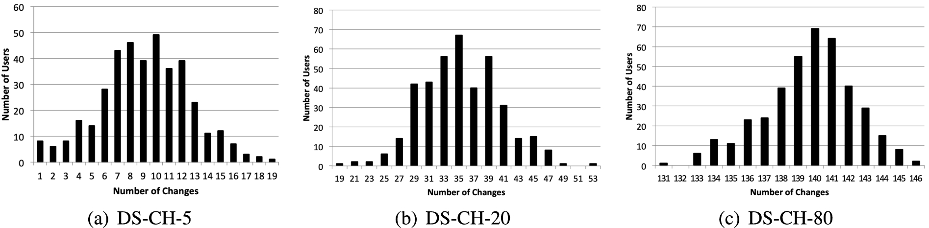
  Distribution of number of users per number of changes.

  As top-k query, we use the one presented in Section 1. We set the length of the window equal to 100 seconds, and the slide equal to 60 seconds. We run 150 iterations of the query evaluation (i.e. we have 150 slided windows for the recorded period of data from twitter) to compare different maintenance policies. The scoring function for each user is a linear combination of the number of mentions (named mn) in the streaming data and the value of $\mathit{dfc}$ in the distributed dataset. Notably the values of mn, and $\mathit{dfc}$ increase or decrease during the iterations, but the selected linear scoring function is monotonic as assumed in top-k query literature. The scoring function computes the score as follows: $$\begin{array}{ll}\hfill \mathit{\text{score}}& =\mathit{F}\mathrm{(}\mathit{m}\mathit{n}\mathrm{,}\mathit{dfc}\mathrm{)}\\ \hfill & ={\mathit{w}}_{\mathit{s}}\ast \mathit{\text{norm}}\mathrm{(}\mathit{m}\mathit{n}\mathrm{)}+{\mathit{w}}_{\mathit{d}}\ast \mathit{\text{norm}}\mathrm{(}\mathit{dfc}\mathrm{)}\mathrm{,}\end{array}$$ where, $\mathit{norm}$ is a function that computes the normalized value of its input, considering the minimum and maximum value in the input range, ${\mathit{w}}_{\mathit{s}}$ is the weight used for the number of mentions, and ${\mathit{w}}_{\mathit{d}}$ in the weight used for the number of followers.

  For experimental evaluation, we need to control the average number of changes in the distributed dataset. Before controlling it, we need to explore the distribution of changes in the recorded data. Notably, Twitter APIs allow asking for the profile of a maximum of 100 users per invocation,10 ¹⁰

  Twitter API returns the information of up to 100 users per request, https://developer.twitter.com/en/docs/accounts-and-users/follow-search-get-users/api-reference/get-users-lookup.

  thus multiple invocations are needed per minutes to get the number of followers and compute the dfc for each of the 400 users. In total, we run 702 invocations to collect the data used over the 150 iterations.

  Exploring the characteristic of the obtained distributed dataset considering dfc, we found that on average, in every invocation of Twitter API, 80 users have changes in dfc.

  Now that we know this information, we generate datasets with a decreased number of changes by sampling the real dataset and randomly decreasing the average number of changes in dfc. To decrease the average number of changes, for each invocation, we randomly select users who have changes in $\mathit{dfc}$ , and set it to the previous value to reach the target average number of changes per invocation.

  We also find that, doing so, we introduce many ties in the scores, which as known in top-k query answering literature simplifies the problem. In order to keep the problem as hard as possible, we alter the changes in dfc by adding random noise.

  Applying those methods, we generate five datasets in which there are on average 5, 10, 20, 40, and 80 changes in each invocation. The value 80 is the maximum number of changes in each invocation for the dataset. So, the dataset with 80 changes in each invocation is the extreme test case that we have in our evaluations. We tested that each generated dataset has normal distribution of the number of changes. We have different mean value for each dataset, but there is not any significant difference between variances. Figure 10 shows the distribution for three of those datasets.

  In order to reduce the risk of bias in synthetic data generation, for each number of changes, we produce a test case that contains 5 different datasets for each number of changes. In the remainder of the paper, we use the notation DS-CH-x to refer collectively to the five datasets whose average number of changes per invocation is equal to x. Table 3 shows the characteristics of the generated datasets. The streaming and distributed datasets, and the implemented experiments are available on GitHub.11 ¹¹

  https://github.com/shima-zahmatkesh/AcquaTop

  Table 3

  Summary of characteristics of distributed datasets which reports the statistic related to the number of changes per invocation

  Dataset	Average	Median	1st Quartile	3rd Quartile
  DS-CH-80	79.97	94	77	96
  DS-CH-40	40.33	47	40	48
  DS-CH-20	20.45	23	20.5	24
  DS-CH-10	10.33	12	10	12
  DS-CH-5	5.53	6	5	6

  6.2. Preliminary experiment

  In this experiment, we check the relevancy and accuracy of the top-k result for all the maintenance policies over 150 iterations. We select DS-CH-20 test case for this experiment. In the first step, we check the total result in each iteration and we found that on average we have got 30 items in the query result. Therefore, we set K equal to 5, which is around 15% of the average size of the total result. We put refresh budget equal to 7, so, theoretically, we have got enough budget to refresh all the answers of the top-k query.

  In order to set parameter N, we have to analyze the distributed datasets. As we say in Section 6.1, during 9462 seconds of recording data from Twitter API, we have 702 invocations. Therefore, on average we have 7.42 invocations per window with 100 seconds length ( $702÷9462\times 100=7.42$ ). We know that in DS-CH-20 test case, we have 20 changes per invocation on average. So, the average number of changes per window is equal to $7.42\times 20=148.4$ . Considering that we have 400 users in total and 30 users on average in the result set, we have 11.13 changes per window ( $\frac{148.4}{400}\times 30=11.13$ ). So, we set the value of N equal to 10 for the MTK+N list.

  In order to investigate our hypotheses, we set up an Oracle that, at each iteration, certainly provides correct answers. Then, we compare the correct answers at iteration i, $\mathit{\text{Ans}}\mathrm{(}{\mathit{Oracle}}_{\mathit{i}}\mathrm{)}$ , with the possibly erroneous ones of the query, $\mathit{\text{Ans}}\mathrm{(}{\mathit{Q}}_{\mathit{i}}\mathrm{)}$ , considering different maintenance policies. Given that the answers are ordered lists of the users’ IDs, we use the metrics presented in Section 2.1.2 to compare the query result with the Oracle one.

  In our experiments, we compute the $\mathit{nDCG}@\mathit{k}$ and $\mathit{precision}@\mathit{k}$ for each iteration of the query evaluation. We also introduce the cumulated $\mathit{nDCG}@\mathit{k}$ ( $\mathit{precision}@\mathit{k}$ ) at the Jth iteration as following: $$\begin{array}{ll}\hfill & \mathit{nDCG}@{\mathit{k}}^{\mathit{C}}\mathrm{(}\mathit{J}\mathrm{)}\\ \hfill & ={\displaystyle \sum }_{\mathit{i}=1}^{\mathit{J}}\mathit{nDCG}@\mathit{k}\mathrm{(}\mathit{\text{Ans}}\mathrm{(}{\mathit{Q}}_{\mathit{i}}\mathrm{)}\mathrm{,}\mathit{\text{Ans}}\mathrm{(}{\mathit{\text{Oracle}}}_{\mathit{i}}\mathrm{)}\mathrm{)}\\ \hfill & \mathit{\text{precision}}@{\mathit{K}}^{\mathit{C}}\mathrm{(}\mathit{J}\mathrm{)}\\ \hfill & ={\displaystyle \sum }_{\mathit{i}=1}^{\mathit{J}}\mathit{\text{precision}}@\mathit{K}\mathrm{(}\mathit{\text{Ans}}\mathrm{(}{\mathit{Q}}_{\mathit{i}}\mathrm{)}\mathrm{,}\mathit{\text{Ans}}\mathrm{(}{\mathit{\text{Oracle}}}_{\mathit{i}}\mathrm{)}\mathrm{)}\end{array}$$ where the $\mathit{nDCG}@\mathit{k}$ of the iteration i is denoted as $\mathit{nDCG}@\mathit{k}\mathrm{(}\mathit{\text{Ans}}\mathrm{(}{\mathit{Q}}_{\mathit{i}}\mathrm{)}\mathrm{,}\mathit{\text{Ans}}\mathrm{(}{\mathit{Oracle}}_{\mathit{i}}\mathrm{)}\mathrm{)}$ and the $\mathit{precision}@\mathit{k}$ of the iteration i as $\mathit{precision}@\mathit{k}\mathrm{(}\mathit{\text{Ans}}\mathrm{(}{\mathit{Q}}_{\mathit{i}}\mathrm{)}\mathrm{,}\mathit{\text{Ans}}\mathrm{(}{\mathit{Oracle}}_{\mathit{i}}\mathrm{)}\mathrm{)}$ . Higher value of $\mathit{nDCG}@\mathit{k}$ and $\mathit{precision}@\mathit{k}$ show more relevancy and accuracy of the result set, respectively.

  
  Fig. 11.

  Result of preliminary experiment.

  We run 150 iterations of query evaluation for each policy and compute the cumulative error related to $\mathit{nDCG}@\mathit{k}$ and $\mathit{precision}@\mathit{k}$ metrics for every iteration. Figure 11 shows the result of the experiment. WST policy has the highest cumulative errors comparing to other policies, which is expected when there is no update in the replica. AT-ASM policy has the lowest error as it updates all the objects in the MTK+N list without considering the limitation of refresh budget. For other policies, in the beginning (iteration 1 to 50) it is difficult to identify policies with better performance, but while the iteration number increases, distinct lines become detectable and comparison between different policies becomes easier. Therefore, for the rest of the experiment, we consider $\mathit{nDCG}@{\mathit{k}}^{\mathit{C}}\mathrm{(}150\mathrm{)}$ , or $\mathit{precision}@{\mathit{k}}^{\mathit{C}}\mathrm{(}150\mathrm{)}$ for comparing the relevancy and accuracy of different policies. Abusing notation, in the rest of the paper, we refer to them using $\mathit{nDCG}@\mathit{k}$ , or $\mathit{precision}@\mathit{k}$ .

  Table 4

  Parameter grid

  Parameter	(Default) Values	Description
  CH	(20) $\{5\mathrm{,}10\mathrm{,}20\mathrm{,}40\mathrm{,}80\}$	Average Number of changes per invocation
  B	(7) $\{1\mathrm{,}3\mathrm{,}5\mathrm{,}7\mathrm{,}10\mathrm{,}15\mathrm{,}20\mathrm{,}25\mathrm{,}30\}$	Refresh budget
  K	(5) $\{5\mathrm{,}7\mathrm{,}10\mathrm{,}15\mathrm{,}20\mathrm{,}30\}$	Number of top-k result
  N	(10) $\{0\mathrm{,}10\mathrm{,}20\mathrm{,}30\mathrm{,}40\}$	Number of additional elements in MTK+N list

  6.3. Research hypotheses

  The space, in which we formulate our hypothesis, has got various dimensions. Table 4 describes them and shows the values for each parameter that we used in the experiments.

  We introduce two baseline maintenance policies (WST, and WSJ-RND) to compare proposed policies with. In WST maintenance policy, we do not have any update of the local replica, so WST policy is a lower bound w.r.t. the comparison in terms of accuracy and relevancy with the Oracle in our experiments.

  WSJ-RND (from [10]) randomly selects objects for updating from the Candidate set. We expect that our proposed policies outperform WSJ-RND policy. As we stated in Section 5.2.3, we also introduce AT-ASM policy as an upper bound. We expect all policies to show worse accuracy and relevancy than AT-ASM w.r.t. Oracle.

  In addition to the baseline policies, we consider WSJ-LRU, and WSJ-WBM policies from ACQUA [10] in order to compare them with our proposed policies. Moreover, as mentioned in Section 5.2.4, we also introduce AT-LRU, and AT-WBM, which use AcquaTop algorithm and Super-MTK+N list, while applying state-of-the-art maintenance policies from ACQUA [10] for updating the local replica.

  In general, we formulate the hypothesis that our proposed policies outperform the state-of-the-art policies within the setting of this paper. As AcquaTop algorithm only keeps the objects which can participate in the top-k result and discards the rest of the data stream, even comparable results with the state-of-the-art policies (WSJ-WBM, and WSJ-LRU) are good. Indeed, AcquaTop algorithm has significant optimization in memory usage, while ACQUA’s memory complexity depends on the amount of data in the window, AcquaTop framework’s memory only depends on K, and N.

  We formulate our hypothesis as follows: