Building relatedness explanations from knowledge graphs

Abstract

Knowledge graphs (KGs) are a key ingredient to complement search results, discover entities and their relations and support several knowledge discovery tasks. We face the problem of building relatedness explanations, that is, graphs that can explain how a pair of entities is related in a KG. Explanations can be used in a variety of tasks; from exploratory search to query answering. We formalize the notion of explanation and present two algorithms. The first, E4D (Explanations from Data), assembles explanations starting from all paths interlinking the source and target entity in the data. The second algorithm E4S (Explanations from Schema) builds explanations focused on a specific relatedness perspective expressed by providing a predicate. E4S first generates candidate explanation patterns at the level of schema; then, it assembles explanations by proceeding to their verification in the data. Given a set of paths, found by E4D or E4S, we describe different criteria to build explanations based on information-theory, diversity, and their combination. As a concrete use-case of relatedness explanations, we introduce relatedness-based KG querying, which revisits the query-by-example paradigm from the perspective of relatedness explanations. We implemented all the machinery in the RECAP tool, which is based on RDF and SPARQL. We discuss an evaluation of the explanation building algorithms and a comparison of RECAP with related systems on real-world data.

Fig. 1.

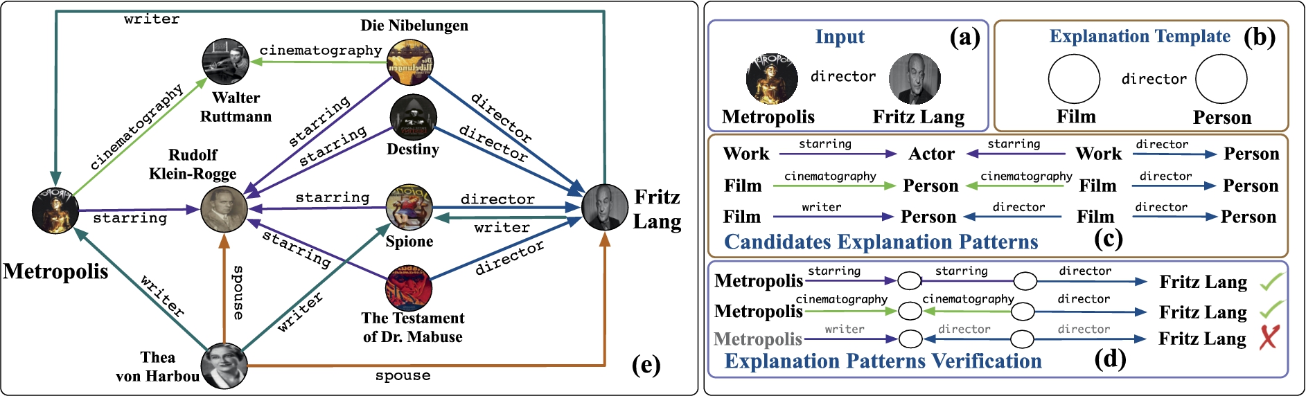
An excerpt of an explanation from the DBpedia KG (left). Overview of the E4S algorithm (right).

1. Introduction

Knowledge graphs (KGs) storing structured data about entities are becoming common support for browsing, searching and knowledge discovery activities [45]. Search engines like Google, Yahoo!, and Bing complement the classical search results with facts about entities in their KGs. An even larger number and variety of KGs, based on the Resource Description Framework (RDF) data format, stem from the Linked Open Data project [23]. DBpedia, Freebase, DBLP, and Yago are just a few examples that witness the popularity and spread of open KGs. KGs are a type of heterogeneous information network [46] where nodes represent entities and edges different types of relationships. Using knowledge from KGs has applications in many domains including information retrieval [28], radicalization detection [43], Twitter analysis [53], recommendation [35], clustering [42], entity resolution [27], and generic exploratory search [39]. One common need for many classes of knowledge discovery tasks is that of explaining the relatedness between entities. The availability of (visual) explanations helps in understanding why entities are related while at the same time allowing to discover/browse other entities of interest. The availability of explanations is useful in several areas including: terrorist networks, to uncover the connections between two suspected terrorists [44]; co-author networks, to discover interlinks between researchers [14]; bioinformatics, to discover relationships between biomedical terms [49]; generic exploratory search [39]. Figure 1(e) shows an excerpt of explanation for the pair of entities (Metropolis, F. Lang) obtained from the DBpedia KG. The explanation includes relationships among entities of different types (e.g., Film, Actors, Cinematographer). We can see that R. Klein-Rogge starred in Metropolis and other films (e.g., Destiny, Spione) all directed by F. Lang. We can also see that T. von Harbou has been married to both R. Klein-Rogge and F.Lang and that she has written some films with the latter. We can also notice that W. Ruttmann has been the cinematographer for both Metropolis and Die Nibelungen. The computation of relatedness explanations is usually tackled by first discovering paths that link entities in the data and then filtering them (e.g., [13,24,29,32,41,47]). Our first explanation-building algorithm called Explanations From the Data (E4D presented in Section 3) [39] follows the same philosophy. However, to guarantee more generality and scalability E4D is SPARQL-based. It reduces the problem of finding paths to that of evaluating a set of (automatically generated) SPARQL queries; thus, it can leverage any SPARQL-enabled (remote) KG. However, working directly at the data level may have some shortcomings. In fact, E4D and related research (e.g., [10,24,47]) do not allow to build focused explanations, that is, explanations concerning a particular relatedness perspective. For pairs of entities interlinked by a larger and semantically diverse number of paths, it can be difficult to identify a precise subset of them that concerns a specific knowledge domain; for instance, explaining the relatedness between a pair of entities by focusing on the domain of movies. Specifying a knowledge domain via one or more target predicates can drive the explanation building process toward data that concern these (and semantically related aspects) only.

To meet these needs, we introduce a second algorithm called Explanations from the Schema (E4S presented in Section 4). The goal is the same as E4D, that is, explaining relatedness between entities with the difference that E4S starts from the KG schema. E4S builds explanation templates given an input target predicate and the entity types of the input pair. This allows building explanations focused on the knowledge domain expressed by the predicate and the entity types. Figure 1(b) shows the explanation template for the entity pair (Metropolis, F. Lang) when considering director as a target predicate. The explanation template is then used to generate candidate explanation patterns, that is, schema-compliant paths having as endpoints entity types (e.g., Film, Person) instead of entity instances (e.g., Metropolis, F. Lang). As the search space for candidate patterns can be very large, E4S leverages a predicate relatedness measure to isolate the portion of the schema that is most related to the target predicate. Figure 1(c) shows some candidate explanation patterns of length 3. These are all plausible ways to link the input pair. We can see for instance, that a Work (Metropolis is a Film, which is a subclassOf Work) has some Actor starring in it. The same Actor starred other Works whose director is a Person. Nevertheless, not all explanation patterns will have a counterpart in the data; they need to be verified to extract knowledge useful to build an explanation. Figure 1(d) shows that only the first two patterns are verified in the data. This can be seen by looking at Fig. 1(e) where we notice that the first pattern leads from Metropolis to F. Lang via R. Klein-Rogge and Spione or Destiny or The Testament of Dr. Mabuse. As for the second pattern, it leads from Metropolis to F. Lang via W. Rotmann and Die Nibelungen. The separation between candidate explanation pattern generation and verification allows choosing only those patterns that are of most interest and proceed to their verification according to some ranking (e.g., average relatedness between predicates in the pattern and target predicate). Focusing on the most interesting explanations first offers a significant advantage wrt related research.

We note that E4D and E4S look at the problem of building explanations from different perspectives. The former builds general explanations by considering all possible paths interlinking a pair of entities while the latter allows building focused explanations by setting a precise relatedness perspective via the input predicate. We are not aware of any previous work that starts from the KG schema to build relatedness explanations.

Contributions. We contribute: (i) a SPARQL-based algorithm called E4D, which starting from a pair of entities can retrieve paths interlinking them directly looking at the data; (ii) a KG-schema-based algorithm E4S, which traverses the schema to build candidate explanation patterns and an algorithm for their verification in the data; (iii) different ways to rank paths (found by E4D or E4S) based on informativeness, diversity and combinations of them; (iv) a (visual) tool called RECAP; (v) an approach to query KGs by relatedness; (vi) an experimental evaluation.

A preliminary version of this work, which does not include the E4S algorithm, appeared in ISWC2015 [39].

Outline. The remainder of the paper is organized as follows. We introduce the problem along with the necessary background in Section 2. Section 3 introduces the E4D algorithm. Section 4 introduces our second algorithm E4S, which builds explanations starting from the KG schema. Section 5 describes different strategies to rank/combine paths in order to build explanations. We describe the RECAP tool implementing our algorithms in Section 6. Section 7 discusses the experimental evaluation. Related Work is treated in Section 8. We conclude in Section 9.

2. Background and problem description

We now introduce the notions of KG and knowledge base. Although there are several KGs today available (e.g., Yahoo!, Google) we will focus on those encoded in RDF1

¹

A list is available at http://lod-cloud.net.

widely and openly accessible on the Web for querying via the standard SPARQL language [22].

Let $\mathcal{U}$ (URIs) and $\mathcal{L}$ (literals) be countably disjoint infinite sets. An RDF triple is a tuple of the form $\mathcal{U}\times \mathcal{U}\times \mathrm{(}\mathcal{U}\cup \mathcal{L}\mathrm{)}$ whose elements are referred to as subject, predicate, and object, respectively. As we are interested in discovering explanations in terms of nodes and edges carrying semantic meaning for the user, we do not consider blank nodes. We also assume an infinite set $\mathcal{V}$ of variables disjoint from the sets $\mathcal{U}$ and  $\mathcal{L}$ . In the SPARQL language, variables in $\mathcal{V}$ are prefixed with a question mark (e.g., $?\mathit{x}$ is a variable).

Definition 1 (Triple and Graph Pattern).

A triple pattern τ is a tuple $\mathrm{(}{\mathit{x}}_{\mathit{s}}\mathrm{,}{\mathit{y}}_{\mathit{p}}\mathrm{,}{\mathit{z}}_{\mathit{o}}\mathrm{)}\in \mathrm{(}\mathcal{U}\cup \mathcal{V}\mathrm{)}Ö\mathrm{(}\mathcal{U}\cup \mathcal{V}\mathrm{)}Ö\mathrm{(}\mathcal{U}\cup \mathcal{L}\cup \mathcal{V}\mathrm{)}$ . We denote by $var\mathrm{(}\mathit{\tau }\mathrm{)}$ the variables in τ. A graph pattern of length k is a set of triple patterns ${\mathit{\tau }}_1\mathrm{,}\dots \mathrm{,}{\mathit{\tau }}_{\mathit{k}}$ where $\mathrm{(}var\mathrm{(}{\mathit{\tau }}_{\mathit{i}}\mathrm{)}\cap var\mathrm{(}{\mathit{\tau }}_{\mathit{i}+1}\mathrm{)}\ne \varnothing \mathrm{)}$ , $\mathit{i}\in [1\mathrm{,}\mathit{k}-1]$ .

A Knowledge Graph (KG) is a node and edge directed labeled multi-graph $\mathit{G}=\mathrm{(}\mathit{V}\mathrm{,}\mathcal{E}\mathrm{,}\mathit{T}\mathrm{)}$ where V is a set of uniquely identified vertices representing entities (e.g., D. Lynch), $\mathcal{E}$ a set of predicates (e.g., director) and T a set of triples of the form (s, p, o) representing directed labeled edges, where s, o $\in \mathit{V}$ and p $\in \mathcal{E}$ .

Fig. 2.

A KG schema (a) and its corresponding schema graph (b).

To structure knowledge, KGs can resort to an underlying schema S, which can be seen as a set of triples defined by using some ontology vocabulary (e.g., RDFS, OWL). In this paper, we focus on RDFS and specifically on entity types (and their hierarchy) and domain and range of predicates. We denote by type(e) the set of types of an entity e and by $\mathit{domain}\mathrm{(}\mathit{p}\mathrm{)}$ (resp., $\mathit{range}\mathrm{(}\mathit{p}\mathrm{)}$ ) the set of nodes (i.e., entity types) in G having an outgoing (resp., incoming) edge labeled with p. Our approach leverages RDFS inference rules to construct the RDFS closure of the KG schema [20,33]. From the closure of the schema, we build the corresponding schema graph.

Definition 2 (Schema Graph).

Given a KG, its schema graph is defined as ${\mathit{G}}_{\mathit{s}}=\mathrm{(}{\mathit{V}}_{\mathit{s}}\mathrm{,}{\mathcal{E}}_{\mathit{s}}\mathrm{,}{\mathit{T}}_{\mathit{s}}\mathrm{)}$ , where each ${\mathit{v}}_{\mathit{i}}\in {\mathit{V}}_{\mathit{s}}$ is a node denoting an entity type, each ${\mathit{p}}_{\mathit{i}}\in {\mathcal{E}}_{\mathit{s}}$ denotes a predicate and each $\mathrm{(}{\mathit{v}}_{\mathit{s}}\mathrm{,}{\mathit{p}}_{\mathit{i}}\mathrm{,}{\mathit{v}}_{\mathit{t}}\mathrm{)}\in {\mathit{T}}_{\mathit{s}}$ is a triple where ${\mathit{v}}_{\mathit{i}}$ (resp., ${\mathit{v}}_{\mathit{t}}$ ) is the domain (resp., range) of the predicate ${\mathit{p}}_{\mathit{i}}$ .

Figure 2(a) shows an excerpt of the DBpedia schema; the figure also shows one of the triples that can be inferred via RDFS reasoning. Fig. 2(b) shows an excerpt of the corresponding schema graph; here, dashed lines represent inferred triples. For instance, the previous triple (Work, director, Person) is inferred from (Film, subclassOf, Work) and (Film, director, Person).

Definition 3 (Knowledge Base).

A knowledge base is a tuple of the form $\mathit{K}=⟨\mathit{G}\mathrm{,}{\mathit{G}}_{\mathit{s}}\mathrm{,}\mathit{A}⟩$ where G is a knowledge graph, ${\mathit{G}}_{\mathit{s}}$ is the schema graph and A is a query endpoint used to access data in G.

2.1. Problem description

Motivation. The high-level objective of this paper is to tackle the problem of explaining relatedness in KGs. In particular, we face the problem of building relatedness explanations, that is, graphs that can shed light on how a pair of entities is interlinked in a KG. This is an important problem in several contexts; for instance, a doctor can be interested in understanding the relationship between a symptom and a disease or a pair of genes; a financial analyst can be interested in finding how a pair of companies is related or to explain the association of a company and supply-chain materials.

The need for relatedness explanations as a knowledge discovery tool also emerged in the context of the SENSE4US FP7 project,2

²

http://www.sense4us.eu

which aimed at creating a toolkit to support information gathering, analysis, and policy modeling. Here, relatedness explanations were useful to investigate and show to the user the topic and entity connectivity. In particular, starting from a set of topics and entities extracted from policy documents, the purpose of explanations was to show to the policy maker how these were connected. As an example, given the entities Renewable energy and Germany, one of the explanations enabled to discover intermediate entities like Senvion, Aleo Solar and Wirsol. The benefit to the policy maker was the possibility to find out previously unknown information (viz., specific German companies in the field of renewable energy) that was of relevance, understand how it was of relevance, and navigate it (e.g., to find details about the company Senvion).

Input. The input of our problem is a pair $\mathrm{(}{\mathit{w}}_{\mathit{s}}\mathrm{,}{\mathit{w}}_{\mathit{t}}\mathrm{)}$ of entities defined in some knowledge base $\mathit{K}=⟨\mathit{G}\mathrm{,}{\mathit{G}}_{\mathit{s}}\mathrm{,}\mathit{A}⟩$ .

Output. Given $\mathit{K}=⟨\mathit{G}\mathrm{,}{\mathit{G}}_{\mathit{s}}\mathrm{,}\mathit{A}⟩$ and a pair of entities $\mathrm{(}{\mathit{w}}_{\mathit{s}}\mathrm{,}{\mathit{w}}_{\mathit{t}}\mathrm{)}$ , the output is a graph ${\mathit{G}}_{\mathit{e}}\subseteq \mathit{G}$ ; we call such a graph the relatedness explanation between ${\mathit{w}}_{\mathit{s}}$ and ${\mathit{w}}_{\mathit{t}}$ .

Challenges. The problem that we tackle in this paper, the algorithmic solutions and their implementation pose several challenges, among which:

how to meaningfully capture the notion of explanation between entities? How to control the size of an explanation? Which kind of information in G is useful for building an explanation?

what role can the KG schema ${\mathit{G}}_{\mathit{s}}$ have?

how to make available the machinery discussed in the paper in a variety of KGs?

2.2. Basic definitions

Before further delving into the discussion of the solutions to the above challenges, we introduce some definitions.

Definition 4 (Explanation).

Given a knowledge graph G and a pair of entities $\mathrm{(}{\mathit{w}}_{\mathit{s}}\mathrm{,}{\mathit{w}}_{\mathit{t}}\mathrm{)}$ where ${\mathit{w}}_{\mathit{s}}\mathrm{,}{\mathit{w}}_{\mathit{t}}\in \mathit{G}$ , an explanation is a tuple of the form $\mathit{E}=\mathrm{(}{\mathit{w}}_{\mathit{s}}\mathrm{,}{\mathit{w}}_{\mathit{t}}\mathrm{,}{\mathit{G}}_{\mathit{e}}\mathrm{)}$ where ${\mathit{w}}_{\mathit{s}}\mathrm{,}{\mathit{w}}_{\mathit{t}}\in {\mathit{G}}_{\mathit{e}}$ and ${\mathit{G}}_{\mathit{e}}\subseteq \mathit{G}$ .

This definition is very general; it only states that two entities are connected via nodes and edges in a graph ${\mathit{G}}_{\mathit{e}}$ , which is a subgraph of the knowledge graph G and has an arbitrary structure. The challenging aspect that we face concerns how to uncover the structure of ${\mathit{G}}_{\mathit{e}}$ . To tackle this challenge, we shall characterize the desired properties of ${\mathit{G}}_{\mathit{e}}$ . Consider the explanation shown in Fig. 3(a); ${\mathit{G}}_{\mathit{e}}$ contains two types of nodes: nodes such as ${\mathit{n}}_1$ , ${\mathit{n}}_3$ , ${\mathit{n}}_4$ that belong to some path between ${\mathit{w}}_{\mathit{s}}$ and ${\mathit{w}}_{\mathit{t}}$ and others (e.g., ${\mathit{n}}_2$ ) that do not.

Fig. 3.

An explanation (a) and a minimal explanation (b).

Although the edge $\mathrm{(}{\mathit{n}}_2\mathrm{,}{\mathit{p}}_1\mathrm{,}{\mathit{n}}_3\mathrm{)}$ can contribute to better characterize ${\mathit{n}}_3$ , such edge is in a sense non-necessary as it does not directly contribute to explain how ${\mathit{w}}_{\mathit{s}}$ and ${\mathit{w}}_{\mathit{t}}$ are related. Hence, we introduce the notion of a necessary edge.

Definition 5 (Necessary Edge).

An edge $\mathrm{(}{\mathit{n}}_{\mathit{i}}\mathrm{,}{\mathit{p}}_{\mathit{k}}\mathrm{,}{\mathit{n}}_{\mathit{j}}\mathrm{)}\in \mathit{G}$ is necessary for an explanation $\mathit{E}=\mathrm{(}{\mathit{w}}_{\mathit{s}}\mathrm{,}{\mathit{w}}_{\mathit{t}}\mathrm{,}{\mathit{G}}_{\mathit{e}}\mathrm{)}$ if it belongs to a simple path (no node repetitions) between ${\mathit{w}}_{\mathit{s}}$ and ${\mathit{w}}_{\mathit{t}}$ .

The necessary edge property enables to refine the notion of explanation into that of minimal explanation.

Definition 6 (Minimal Explanation).

Given a knowledge graph G and a pair of entities $\mathrm{(}{\mathit{w}}_{\mathit{s}}\mathrm{,}{\mathit{w}}_{\mathit{t}}\mathrm{)}$ where ${\mathit{w}}_{\mathit{s}}\mathrm{,}{\mathit{w}}_{\mathit{t}}\in \mathit{G}$ , a minimal explanation is an explanation $\mathit{E}=\mathrm{(}{\mathit{w}}_{\mathit{s}}\mathrm{,}{\mathit{w}}_{\mathit{t}}\mathrm{,}{\mathit{G}}_{\mathit{e}}\mathrm{)}$ where ${\mathit{G}}_{\mathit{e}}$ is obtained as the merge of all simple paths between ${\mathit{w}}_{\mathit{s}}$ and ${\mathit{w}}_{\mathit{t}}$ .

Figure 3(b) shows a minimal explanation. Minimal explanations enable to focus only on nodes and edges that are in some path between ${\mathit{w}}_{\mathit{s}}$ and ${\mathit{w}}_{\mathit{t}}$ ; hence, minimal explanations preserve reachability information only. Representing explanations as graphs enables users to have (visual) insights of why/how two entities are related and discover/browse other entities. An investigation of the usefulness of graph visualization supports is out of the scope of this paper; the reader can refer to Herman et al. [26] for a comprehensive discussion about the topic. We are now ready to introduce our first algorithm, which discovers paths useful to build different kinds of relatedness explanations by directly looking at the KG data.

3. Explaining relatedness from the data (E4D)

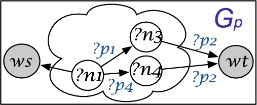
Relatedness explanations are graphs that provide a (concise) representation of the relatedness between a pair of entities in a KG in terms of predicates (carrying a semantic meaning) and other entities. The challenging question is how to retrieve explanations. Consider the minimal explanation shown in Fig. 3(b); it could be retrieved by matching the pattern graph ${\mathit{G}}_{\mathit{p}}$ shown in Fig. 4 (nodes and edges are query variables) against G. Hence, if the structure of ${\mathit{G}}_{\mathit{p}}$ were available one could easily find ${\mathit{G}}_{\mathit{e}}$ ; however, such structure, that is, the right way of joining query variables representing nodes and edges in ${\mathit{G}}_{\mathit{p}}$ is unknown before knowing ${\mathit{G}}_{\mathit{e}}$ . Nevertheless, since minimal explanations are built by considering (simple) paths in the data between ${\mathit{w}}_{\mathit{s}}$ and ${\mathit{w}}_{\mathit{t}}$ , the retrieval of such paths is the first step toward building explanations via the E4D (Explanations from the Data) algorithm.

Fig. 4.

The pattern graph for the minimal explanation in Fig. 3(b).

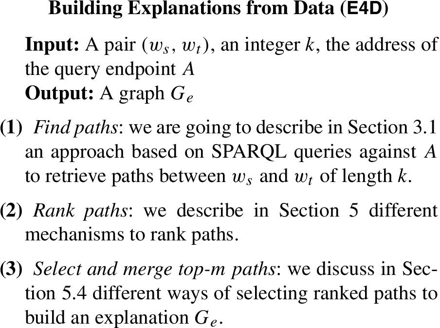
Generally speaking, paths between entities can have an arbitrary length; in practice, it has been shown that for KGs like Facebook the average distance between entities is bound by a value [50]. The choice of considering paths of length k in our approach is reasonable on the light of the fact that we focus on providing explanations of manageable size that can be visualized and interpreted by the user. Figure 5 outlines our first explanation building approach.

Fig. 5.

Building explanations from the data.

We now describe step (1); step (2) and (3) will be described in Section 5.

3.1. Finding paths from the data

A path is a sequence of edges (RDF triples) bound by a length value k. The underlying assumption of the E4D algorithm is to query data via the query endpoint A only. This allows to work on top of any SPARQL-enabled KG thus making the approach readily usable in a variety of domains and without the need to set up custom infrastructures in terms of storage and computing power.

Definition 7 (k-connectivity Pattern).

Given a knowledge graph G, a pair of entities $\mathrm{(}{\mathit{w}}_{\mathit{s}}\mathrm{,}{\mathit{w}}_{\mathit{t}}\mathrm{)}$ where ${\mathit{w}}_{\mathit{s}}\mathrm{,}{\mathit{w}}_{\mathit{t}}\in \mathit{G}$ and an integer k, a k-connectivity pattern is a tuple of the form $\mathrm{\Xi }=⟨{\mathit{w}}_{\mathit{s}}\mathrm{,}{\mathit{w}}_{\mathit{t}}\mathrm{,}\mathcal{T}\mathrm{,}\mathit{k}⟩$ where $\mathcal{T}$ is a graph pattern of length k.

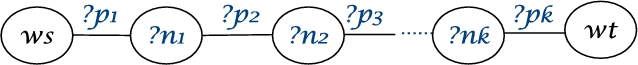
An example of graph pattern $\mathcal{T}$ is shown in Fig. 6. Here, both nodes (but ${\mathit{w}}_{\mathit{s}}$ and ${\mathit{w}}_{\mathit{t}}$ ) and edges represent query variables. Note that in the figure, edge directions are not reported; each edge has to be considered both as incoming and outgoing, which corresponds to join triple patterns in all possible ways. Indeed, by joining each of the k triple patterns in Fig. 6 in all different ways it is possible to obtain a set of $2^{\mathit{k}}$ graph patterns. These patterns are used to generate SPARQL queries.

Fig. 6.

Structure of a query to find paths of length k.

Example 8 (Example of k-connectivity Pattern).

The 2-connectivity pattern between Metropolis (:Mt) and F. Lang (:FL) allows generating the following set of 4 queries:

As we are going to discuss in the following, these queries are executed in parallel (by using multithreading) by E4D thus significantly speeding up the retrieval of paths. Note that SPARQL 1.1 supports property paths (PPs) [19,22], that is, a way to discover routes between nodes in an RDF graph. However, since variables cannot be used as part of the path specification itself, PPs are not suitable for our purpose; we need information about all the constituent elements of a path (both nodes and edges) to build explanations.

Definition 9 (Path).

Given a graph G and a pair of entities $\mathrm{(}{\mathit{w}}_{\mathit{s}}\mathrm{,}{\mathit{w}}_{\mathit{t}}\mathrm{)}$ , a path ξ is a set of edges (i.e., RDF triples): $\mathit{\xi }\mathrm{(}{\mathit{w}}_{\mathit{s}}\mathrm{,}{\mathit{w}}_{\mathit{t}}\mathrm{)}={\mathit{w}}_{\mathit{s}}\stackrel{{\mathit{p}}_1}{-}{\mathit{n}}_1\stackrel{{\mathit{p}}_2}{-}{\mathit{n}}_2\stackrel{{\mathit{p}}_3}{-}{\mathit{n}}_3..{\mathit{n}}_{\mathit{d}}\stackrel{{\mathit{p}}_{\mathit{k}}}{-}{\mathit{w}}_{\mathit{t}}$ , ${\mathit{n}}_{\mathit{i}}\in \mathit{G}$ $\forall \mathit{i}\in [1\mathrm{,}\mathit{d}]$ , ${\mathit{p}}_{\mathit{j}}\in \mathit{G}$ $\forall \mathit{j}\in [1\mathrm{,}\mathit{k}]$ and $-\in \{\leftarrow \mathrm{,}\to \}$ .

In the above definition, the symbol − models the fact that in a path we may have edges pointing in different directions. We denote by Lab(ξ) the set of labels (RDF predicates) in ξ.

Fig. 7.

An example of path between Metropolis and F. Lang.

Fig. 8.

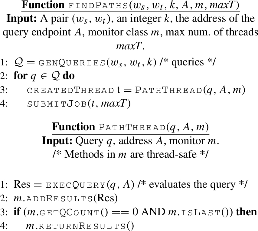
Finding paths: an overview.

Practically speaking, paths are obtained by evaluating queries deriving from a k-connectivity pattern; hence, ${\mathit{n}}_{\mathit{i}}$ and ${\mathit{p}}_{\mathit{j}}$ are solutions (variable bindings) obtained from some query evaluated on A. While in a k-connectivity pattern all edges and nodes (but ${\mathit{w}}_{\mathit{s}}$ and ${\mathit{w}}_{\mathit{t}}$ ) are variables, in a path, there are no variables. Fig. 7 shows an example of path ξ where Lab(ξ) = {writer, spouse}. We want to stress the fact that the set of queries to retrieve paths are automatically generated and evaluated on the (remote) query endpoint A. A sketch of the multithread algorithm to find paths is shown in Fig. 8. The algorithm leverages a monitor class (not reported here); an instance of such class is denoted with m in the pseudocode. This class controls: (i) the concurrent access to the shared data structures by the threads (e.g., to add paths retrieved by queries); (ii) the termination of the algorithm that will happen when no more queries have to be executed and no thread is active (see lines 3–4 PathThread). Moreover, the method submitJob (not reported here) takes care of submitting threads for the executions to an executor service, which can be configured to create a maxT number of threads. This enables to control the degree of concurrency.

We now move to the description of the E4S algorithm, which adopts a different philosophy; instead of starting from the evaluation of queries directly in the KG data to obtain all paths between ${\mathit{w}}_{\mathit{s}}$ and ${\mathit{w}}_{\mathit{t}}$ , it leverages the schema to filter paths according to a specific relatedness perspective.

4. Explaining relatedness from the schema (E4S)

E4D can lead to a potentially large and semantically varied number of paths. In some contexts, one may be interested in the generation of explanations focused on a specific relatedness perspective. As an example, when explaining the relatedness between the film Metropolis and F. Lang one could focus on explanations in the domain of movies.

To meet this requirement, we now introduce the E4S (Explaining Relatedness from the Schema) algorithm, which builds domain-driven explanations. The target domain is expressed by using predicates available in the KG schema. For instance, explanations in the domain of movies can be sought by giving as input predicates like director, actor or writer. From an algorithmic point of view, E4S leverages the domain-specific input predicate to restrict the portion of the KG accessed.

Definition 10 (Explanation Template).

Given a knowledge base $\mathit{K}=⟨\mathit{G}\mathrm{,}{\mathit{G}}_{\mathit{s}}\mathrm{,}\mathit{A}⟩$ , a source entity ${\mathit{w}}_{\mathit{s}}\in \mathit{G}$ , a target entity ${\mathit{w}}_{\mathit{t}}\in \mathit{G}$ , a schema graph ${\mathit{G}}_{\mathit{s}}=\mathrm{(}{\mathit{V}}_{\mathit{s}}\mathrm{,}{\mathcal{E}}_{\mathit{s}}\mathrm{,}{\mathit{T}}_{\mathit{s}}\mathrm{)}$ and a target predicate ${\mathit{p}}^{\ast }\in {\mathcal{E}}_{\mathit{s}}$ , an explanation template is a triple $\mathrm{(}\mathit{x}\mathrm{,}{\mathit{p}}^{\ast }\mathrm{,}\mathit{z}\mathrm{)}$ where $\mathit{x}\in \mathit{domain}\mathrm{(}{\mathit{p}}^{\ast }\mathrm{)}$ and $\mathit{z}\in \mathit{range}\mathrm{(}{\mathit{p}}^{\ast }\mathrm{)}$ .

Explanation templates are the building blocks of explanation patterns.

Definition 11 (Explanation Pattern).

Given a schema graph ${\mathit{G}}_{\mathit{s}}=\mathrm{(}{\mathit{V}}_{\mathit{s}}\mathrm{,}{\mathcal{E}}_{\mathit{s}}\mathrm{,}{\mathit{T}}_{\mathit{s}}\mathrm{)}$ , an explanation template $\mathrm{(}{\mathit{x}}_1\mathrm{,}{\mathit{p}}^{\ast }\mathrm{,}{\mathit{x}}_{\mathit{d}}\mathrm{)}$ and an integer d, an explanation pattern is $\mathbf{T}\mathrm{(}{\mathit{p}}^{\ast }\mathrm{)}={\mathit{x}}_1\stackrel{{\mathit{p}}_1}{-}{\mathit{x}}_2\stackrel{{\mathit{p}}_2}{-}{\mathit{x}}_3\stackrel{{\mathit{p}}_3}{-}{\mathit{x}}_3..{\mathit{x}}_{\mathit{d}}\stackrel{{\mathit{p}}_{\mathit{d}}}{-}{\mathit{x}}_{\mathit{d}+1}$ where ${\mathit{x}}_{\mathit{i}}\in {\mathit{V}}_{\mathit{s}}$ $\forall \mathit{i}\in [1\mathrm{,}\mathit{d}+1]$ , ${\mathit{p}}_{\mathit{j}}\in {\mathcal{E}}_{\mathit{s}}$ $\forall \mathit{j}\in [1\mathrm{,}\mathit{d}]$ and $-\in \{\leftarrow \mathrm{,}\to \}$ .

By looking at Fig. 2(b), an example of explanation pattern is T(director) = Work $\stackrel{\mathsf{\text{starring}}}{\to }$ Actor $\stackrel{\mathsf{\text{starring}}}{\leftarrow }$ Work  $\stackrel{\mathsf{\text{director}}}{\leftarrow }$ Person). As it can be noted, this explanation pattern only contains predicates that are semantically related to the target predicate, that is, director. Figure 9 gives an overview of the step performed by the E4S algorithm to build relatedness explanations. Note that while E4D builds explanations by considering all possible relatedness perspectives (all paths), E4S sets a precise relatedness perspective via the input predicate.

Fig. 9.

Building explanations from the schema.

Table 1

Examples of related predicates in DBpedia

director	writer	spouse	influenced	birthPlace
writer	producer	child	influencedBy	deathPlace
producer	director	relative	author	residence
musicComposer	musicComposer	parent	notableWork	country
executiveProducer	composer	relation	spouse	restingPlace
starring	author	starring	child	hometown

4.1. Predicate relatedness

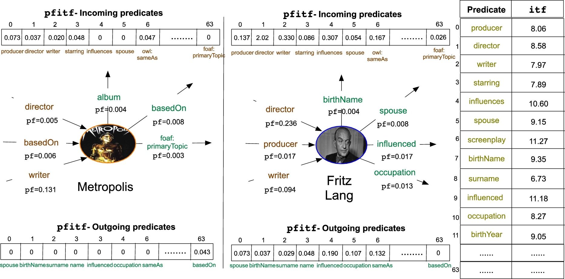
The first ingredient of the E4S algorithm is a predicate relatedness measure, which given a target predicate ${\mathit{p}}^{\ast }$ allows focusing on the part of the schema most related to ${\mathit{p}}^{\ast }$ during the candidate explanation generation, and thus of the data during candidate verification. Given a knowledge graph $\mathit{G}=\mathrm{(}\mathit{V}\mathrm{,}\mathcal{E}\mathrm{,}\mathit{T}\mathrm{)}$ and a pair of predicates $\mathrm{(}{\mathit{p}}_{\mathit{i}}\mathrm{,}{\mathit{p}}_{\mathit{j}}\mathrm{)}\in \mathcal{E}$ , the relatedness measure takes into account the co-occurrence of ${\mathit{p}}_{\mathit{i}}$ and ${\mathit{p}}_{\mathit{j}}$ in the set of triples T and weights it by the predicate popularity [18,38]. This approach resembles the TF-ITF method used in information retrieval to weight the importance of words in documents. We now introduce the building blocks of the predicated relatedness measure, starting from the Term Frequency $TF\mathrm{(}{\mathit{p}}_{\mathit{i}}\mathrm{,}{\mathit{p}}_{\mathit{j}}\mathrm{)}$ . $$\begin{array}{}\text{(1)}& TF\mathrm{(}{\mathit{p}}_{\mathit{i}}\mathrm{,}{\mathit{p}}_{\mathit{j}}\mathrm{)}=log\mathrm{(}1+{\mathit{C}}_{\mathit{i}\mathrm{,}\mathit{j}}\mathrm{)}\end{array}$$ In the above formula, ${\mathit{C}}_{\mathit{i}\mathrm{,}\mathit{j}}$ counts the number of subjects (s) and objects (o) in triples of the form $\mathrm{(}\mathit{s}\mathrm{,}{\mathit{p}}_{\mathit{i}}\mathrm{,}\mathit{o}\mathrm{)}$ , and $\mathrm{(}\mathit{s}\mathrm{,}{\mathit{p}}_{\mathit{j}}\mathrm{,}\mathit{o}\mathrm{)}$ or $\mathrm{(}\mathit{o}\mathrm{,}{\mathit{p}}_{\mathit{i}}\mathrm{,}\mathit{s}\mathrm{)}$ and $\mathrm{(}\mathit{o}\mathrm{,}{\mathit{p}}_{\mathit{j}}\mathrm{,}\mathit{s}\mathrm{)}$ . The Inverse Term Frequency (ITF) is defined as follows: $$\begin{array}{}\text{(2)}& ITF\mathrm{(}{\mathit{p}}_{\mathit{j}}\mathrm{,}\mathcal{E}\mathrm{)}=log{\displaystyle \frac{|\mathcal{E}|}{|\{{\mathit{p}}_{\mathit{i}}:{\mathit{C}}_{\mathit{i}\mathrm{,}\mathit{j}}\mathrm{>}0\}|}}\end{array}$$ Having co-occurrences for each pair $\mathrm{(}{\mathit{p}}_{\mathit{i}}\mathrm{,}{\mathit{p}}_{\mathit{j}}\mathrm{)}$ weighted by the ITF allows to build a co-occurrence matrix with entries defined as follows: $$\begin{array}{}\text{(3)}& {\mathit{w}}_{\mathit{i}\mathrm{,}\mathit{j}}\mathrm{(}{\mathit{p}}_{\mathit{i}}\mathrm{,}{\mathit{p}}_{\mathit{j}}\mathrm{,}\mathcal{E}\mathrm{)}=TF\mathrm{(}{\mathit{p}}_{\mathit{i}}\mathrm{,}{\mathit{p}}_{\mathit{j}}\mathrm{)}\times ITF\mathrm{(}{\mathit{p}}_{\mathit{j}}\mathrm{,}\mathcal{E}\mathrm{)}\end{array}$$ At this point, the relatedness between ${\mathit{p}}_{\mathit{i}}$ and ${\mathit{p}}_{\mathit{j}}$ can be computed by looking at their relative rows as: $$\begin{array}{}\text{(4)}& Rel\mathrm{(}{\mathit{p}}_{\mathit{i}}\mathrm{,}{\mathit{p}}_{\mathit{j}}\mathrm{)}=Cosine\mathrm{(}{\mathit{W}}_{\mathit{i}}\mathrm{,}{\mathit{W}}_{\mathit{j}}\mathrm{)}\end{array}$$ where ${\mathit{W}}_{\mathit{i}}$ (resp., ${\mathit{W}}_{\mathit{j}}$ ) is the row of ${\mathit{p}}_{\mathit{i}}$ (resp., ${\mathit{p}}_{\mathit{j}}$ ).

To give some hint about the results obtained by the predicate relatedness measure, Table 1 shows the top-5 most related predicates when giving as input some predicates (in bold) defined in the DBpedia ontology. We can see, for instance, that director is very related to writer and producer; that spouse is very related to child and relative and so forth. The predicate relatedness measure seems to reasonably output semantically related predicates given a target predicate.

4.2. Finding candidate explanation patterns

We now describe how the E4S algorithm generates candidate explanation patterns. This process is handled via Algorithm 1, which takes as input a schema graph, a target predicate ${\mathit{p}}^{\ast }$ , an integer d to restrict the length of the pattern, an integer k to pick the top-k most related predicates to ${\mathit{p}}^{\ast }$ , and uses a priority queue to store candidate explanation patterns ranked by their relatedness wrt the target predicate ${\mathit{p}}^{\ast }$ .

Algorithm 1:

findCandidateExplPatterns

The algorithm for each of the most related predicates (line 4) runs in parallel a traversal of the schema graph by checking that predicate ${\mathit{p}}_{\mathit{i}}$ and predicate ${\mathit{p}}^{\ast }$ both have as source node ${\mathit{t}}_{\mathit{r}}$ (line 7) (resp., ${\mathit{t}}_{\mathit{s}}$ (line 13)); this allows building length-1 explanation patterns that are added to the results if they allow to reach the same node ${\mathit{t}}_{\mathit{s}}$ (line 9) (resp., ${\mathit{t}}_{\mathit{r}}$ (line 15)). Length-1 explanation patterns are possibly expanded; the algorithm takes a q-length (partial) pattern (with $\mathit{q}\mathrm{<}\mathit{d}$ ) and expands it by only considering the top-k most related predicates to ${\mathit{p}}^{\ast }$ (lines 22 and 24). The expansion is done both in forward and reverse direction as the schema graph is treated as undirected. Candidate explanation patterns of at most length d are added to the results (line 34) after checking that the pattern starts from one of the nodes in $\mathit{domain}\mathrm{(}{\mathit{p}}^{\ast }\mathrm{)}$ and ends in one of the nodes in $\mathit{range}\mathrm{(}{\mathit{p}}^{\ast }\mathrm{)}$ (line 33). The algorithm runs (in parallel) a d-step traversal of the graph and at each step at most $|{\mathit{E}}_{\mathit{s}}|$ edges (note that the algorithm in practice considers a subset R of all predicates) can be visited. checkTypes can be done in constant time by hashing domain(s) and range(s) of predicates.

4.3. Verifying explanation patterns

Candidate explanation patterns found via Algorithm 1 represent schema-compliant ways in which type( ${\mathit{w}}_{\mathit{s}}$ ) (viz., $\mathit{domain}\mathrm{(}{\mathit{p}}^{\ast }\mathrm{)}$ ) and type( ${\mathit{w}}_{\mathit{s}}$ ) (viz., $\mathit{range}\mathrm{(}{\mathit{p}}^{\ast }\mathrm{)}$ ) could be connected in the underlying data.

To understand which explanation patterns actually contribute to build a relatedness explanation there is the need to verify them. A pattern is verified if starting from ${\mathit{w}}_{\mathit{s}}$ it is possible to reach ${\mathit{w}}_{\mathit{t}}$ by traversing the sequence of edges in it. In other words, to verify a pattern we need to instantiate its endpoints with ${\mathit{w}}_{\mathit{s}}$ and ${\mathit{w}}_{\mathit{t}}$ and then check if it has a solution in the data.

As an example, by instantiating the first explanation pattern in Fig. 1(c), we obtain the explanation pattern in Fig. 1(d). This pattern is actually verified as can be seen in Fig. 1(e). On the other hand, the last one is not verified. We now outline our approach for candidate patterns verification, which builds upon the notion of path pattern.

Definition 12 (Path Pattern).

Given a source entity ${\mathit{w}}_{\mathit{s}}$ a target entity ${\mathit{w}}_{\mathit{t}}$ and a candidate explanation pattern $\mathbf{T}\mathrm{(}{\mathit{p}}^{\ast }\mathrm{)}={\mathit{x}}_1\stackrel{{\mathit{p}}_1}{-}{\mathit{x}}_2\stackrel{{\mathit{p}}_2}{-}{\mathit{x}}_3\stackrel{{\mathit{p}}_3}{-}{\mathit{x}}_3..{\mathit{x}}_{\mathit{d}}\stackrel{{\mathit{p}}_{\mathit{d}}}{-}{\mathit{x}}_{\mathit{d}+1}$ , its corresponding path pattern is: $\mathrm{\Pi }\mathrm{(}{\mathit{w}}_{\mathit{s}}\mathrm{,}{\mathit{w}}_{\mathit{t}}\mathrm{,}\mathbf{T}\mathrm{(}{\mathit{p}}^{\ast }\mathrm{)}\mathrm{)}={\mathit{\tau }}_1.{\mathit{\tau }}_2\mathrm{,}\dots \mathrm{,}{\mathit{\tau }}_{\mathit{d}}$ where ${\mathit{\tau }}_1={\mathit{w}}_{\mathit{s}}{\mathit{p}}_1?{\mathit{v}}_2$ (resp., $?{\mathit{v}}_2{\mathit{p}}_1{\mathit{w}}_{\mathit{s}}$ ) if $\stackrel{{\mathit{p}}_1}{-}=\stackrel{{\mathit{p}}_1}{\to }$ (resp., $\stackrel{{\mathit{p}}_1}{-}=\stackrel{{\mathit{p}}_1}{\leftarrow }$ ), ${\mathit{\tau }}_{\mathit{i}}=?{\mathit{v}}_{\mathit{i}}{\mathit{p}}_{\mathit{i}}?{\mathit{v}}_{\mathit{i}+1}$ (resp., $?{\mathit{v}}_{\mathit{i}+1}{\mathit{p}}_{\mathit{i}}?{\mathit{v}}_{\mathit{i}}$ ) if $\stackrel{{\mathit{p}}_{\mathit{i}}}{-}=\stackrel{{\mathit{p}}_{\mathit{i}}}{\to }$ (resp., $\stackrel{{\mathit{p}}_{\mathit{i}}}{-}=\stackrel{{\mathit{p}}_{\mathit{i}}}{\leftarrow }$ ) for $2\mathrm{<}\mathit{i}\mathrm{<}\mathit{d}$ , ${\mathit{\tau }}_{\mathit{d}}=?{\mathit{v}}_{\mathit{d}}{\mathit{p}}_{\mathit{d}}{\mathit{w}}_{\mathit{t}}$ (resp., ${\mathit{w}}_{\mathit{t}}{\mathit{p}}_{\mathit{d}}?{\mathit{v}}_{\mathit{d}}$ ) if $\stackrel{{\mathit{p}}_{\mathit{d}}}{-}=\stackrel{{\mathit{p}}_{\mathit{d}}}{\to }$ (resp., $\stackrel{{\mathit{p}}_{\mathit{d}}}{-}=\stackrel{{\mathit{p}}_{\mathit{d}}}{\leftarrow }$ ); here, $?{\mathit{v}}_{\mathit{i}}$ are query variables and . denote the join operator.

A path pattern basically transforms a candidate explanation pattern into a SPARQL graph pattern [37] where individual triple patterns are joined (via.) thanks to shared variables, and the endpoints are replaced with the source ( ${\mathit{w}}_{\mathit{s}}$ ) and target entity ( ${\mathit{w}}_{\mathit{t}}$ ). Note that an additional triple pattern can be used to check that, for each triple pattern, the bindings (viz. entities in the KG) of the variable $?{\mathit{v}}_{\mathit{i}}$ are of the right type. As an example, given the pair (Metropolis, F. Lang) and the candidate explanation pattern T(director) = Work $\stackrel{\mathsf{\text{starring}}}{\to }$ Actor $\stackrel{\mathsf{\text{starring}}}{\leftarrow }$ Work $\stackrel{\mathsf{\text{director}}}{\leftarrow }$ Person), by enforcing the type constraint we obtain the path pattern Π(Metropolis, F. Lang, T(director)) = Metropolis starring $?{\mathit{v}}_1$ . $?{\mathit{v}}_1$ type Actor. $?{\mathit{v}}_2$ starring $?\mathit{v}1$ . $?{\mathit{v}}_2$ type Work. $?\mathit{v}2$ directorF. Lang.

4.3.1. Building a SPARQL query for the verification

At this point, from a path pattern, we can build a SPARQL query whose evaluation allows checking whether the original candidate explanation pattern is verified and, if so, to get a set of paths that conform to it. The prototypical SPARQL query has the form:

As an example, the SPARQL query obtained from the path pattern Π(Metropolis, F. Lang, T(director)) when also enforcing intermediate type constraints, is:

E4S has the advantage of requiring the evaluation of SPARQL queries more specific than those required by E4D as predicates are fixed (i.e., there are no variables in the predicate position of triple patterns) and the bindings of variables can be forced to be of specific types. Moreover, note that since candidate explanation patterns work at the level of schema, they do not need to be generated from scratch; they can be reused when the target predicate is the same.

5. Ranking paths to build explanations

We have described two different algorithms to find paths connecting two entities ${\mathit{w}}_{\mathit{s}}$ and ${\mathit{w}}_{\mathit{t}}$ in a KG. In both cases, we may have that the number of such paths can be prohibitively large, which can hinder the process of making sense of an explanation. As an example, considering the merge of all paths, as done in minimal explanations (see Definition 6) may be an obstacle toward providing concise explanations to the users. To cope with this issue, we are going to introduce different criteria to rank paths. Having a rank among paths gives flexibility in choosing the set of paths that will form an explanation. Cheng et al. provide an overview of the topic [9].

Fig. 10.

An example of pfitf computation.

5.1. Path informativeness

The first approach to rank paths leverages the notion of informativeness. Given a graph G, the informativeness of a path connecting a pair of entities $\mathrm{(}{\mathit{w}}_{\mathit{s}}\mathrm{,}{\mathit{w}}_{\mathit{t}}\mathrm{)}\in \mathit{G}$ is estimated by investigating the informativeness of its constituent RDF predicates. This reasoning is analogous to that of associating relative importance to words in a document [6] contained in a set of documents. We leverage the notion of Predicate Frequency Inverse Triple Frequency (pfitf) [38].

Definition 13 (Predicate Frequency).

Given a knowledge graph $\mathit{G}=\mathrm{(}\mathit{V}\mathrm{,}\mathcal{E}\mathrm{,}\mathit{T}\mathrm{)}$ , an entity $\mathit{w}\in \mathit{V}$ and a predicate $\mathit{p}\in \mathcal{E}$ appearing in some triple involving w, the Predicate Frequency ( $\mathtt{\text{pf}}$ ) quantifies the informativeness of p wrt w.

We distinguish between incoming ${\mathtt{\text{pf}}}_{\mathit{i}}^{\mathit{w}}\mathrm{(}\mathit{p}\mathrm{)}$ and outgoing ${\mathtt{\text{pf}}}_{\mathit{o}}^{\mathit{w}}\mathrm{(}\mathit{p}\mathrm{)}$ : $$\begin{array}{}\text{(5)}& {\mathtt{\text{pf}}}_{\mathit{i}}^{\mathit{w}}\mathrm{(}\mathit{p}\mathrm{,}\mathit{G}\mathrm{)}={\displaystyle \frac{|{\mathit{T}}_{\mathit{i}}{|}_{|\mathit{p}}}{|{\mathit{T}}_{\mathit{i}}|}}\text{(6)}& {\mathtt{\text{pf}}}_{\mathit{o}}^{\mathit{w}}\mathrm{(}\mathit{p}\mathrm{,}\mathit{G}\mathrm{)}={\displaystyle \frac{|{\mathit{T}}_{\mathit{o}}{|}_{|\mathit{p}}}{|{\mathit{T}}_{\mathit{o}}|}}\end{array}$$ where $|{\mathit{T}}_{\mathit{i}}{|}_{|\mathit{p}}$ (resp., $|{\mathit{T}}_0{|}_{|\mathit{p}}$ ) is the number of triples in G where the predicate p is incoming (resp., outgoing) in w and $|{\mathit{T}}_{\mathit{i}}|$ (resp., $|{\mathit{T}}_{\mathit{o}}|$ ) is the total number of incoming (resp., outgoing) triples in which w is involved.

Definition 14 (Inverse Triple Frequency).

Given $\mathit{G}=\mathrm{(}\mathit{V}\mathrm{,}\mathcal{E}\mathrm{,}\mathit{T}\mathrm{)}$ and a predicate $\mathit{p}\in \mathcal{E}$ , the inverse triple frequency of p, denoted by $\mathtt{\text{itf}}\mathrm{(}\mathit{p}\mathrm{)}$ , is defined as: $$\begin{array}{}\text{(7)}& \mathtt{\text{itf}}\mathrm{(}\mathit{p}\mathrm{,}\mathit{G}\mathrm{)}=log{\displaystyle \frac{|\mathit{T}|}{|\mathit{T}{|}_{|\mathit{p}}}}\end{array}$$ where $|\mathit{T}|$ is the total number of triples in G and $|\mathit{T}{|}_{|\mathit{p}}$ the total number of triples containing p.

Definition 15 (Predicate Frequency Inverse Triple Frequency).

The Predicate Frequency Inverse Triple Frequency is defined as $\mathtt{\text{pfitf}}\mathrm{(}\mathit{p}\mathrm{,}\mathit{G}\mathrm{)}=\mathtt{\text{pf}}\times \mathtt{\text{itf}}$ . One can consider the incoming ${\mathtt{\text{pfitf}}}_{\mathit{i}}\mathrm{(}\mathit{p}\mathrm{,}\mathit{G}\mathrm{)}={\mathtt{\text{pf}}}_{\mathit{i}}\times \mathtt{\text{itf}}$ and outgoing ${\mathtt{\text{pfitf}}}_{\mathit{o}}\mathrm{(}\mathit{p}\mathrm{,}\mathit{G}\mathrm{)}={\mathtt{\text{pf}}}_{\mathit{i}}\times \mathtt{\text{itf}}$ case.

An example of pfitf computation is shown in Fig. 10. Having a way to assess the relative informativeness of a predicate wrt to an entity in a path, we can now define the informativeness of a path.

Definition 16 (Path Informativeness).

Consider a path $\mathit{\xi }={\mathit{w}}_{\mathit{s}}\stackrel{{\mathit{p}}_1}{-}{\mathit{e}}_1\stackrel{{\mathit{p}}_2}{-}{\mathit{e}}_2\stackrel{{\mathit{p}}_3}{-}{\mathit{e}}_3..{\mathit{e}}_{\mathit{d}}\stackrel{{\mathit{p}}_{\mathit{k}}}{-}{\mathit{w}}_{\mathit{t}}\dots$ of length k.

For $\mathit{k}=1$ , the informativeness of ξ is: $$\begin{array}{}\text{(8)}& \mathit{I}\mathrm{(}\mathit{\xi }\mathrm{,}\mathit{G}\mathrm{)}=[{\mathtt{\text{pfitf}}}_{\mathit{o}}^{{\mathit{w}}_{\mathit{s}}}\mathrm{(}{\mathit{p}}_1\mathrm{)}+{\mathtt{\text{pfitf}}}_{\mathit{i}}^{{\mathit{e}}_1}\mathrm{(}{\mathit{p}}_1\mathrm{)}]\mathrm{/}2\end{array}$$ It considers the predicate ${\mathit{p}}_1$ as outgoing from ${\mathit{w}}_1$ and incoming to ${\mathit{e}}_1$ . The second case for $\mathit{k}=1$ is $\mathit{\xi }\mathrm{(}{\mathit{w}}_1\mathrm{,}{\mathit{e}}_1\mathrm{)}={\mathit{w}}_1\stackrel{\mathit{p}}{⟵}{\mathit{e}}_1$ where ${\mathit{p}}_1$ is an incoming edge for ${\mathit{w}}_1$ and outgoing from ${\mathit{e}}_1$ and can be treated in a similar way. For paths of length $\mathit{k}\mathrm{>}1$ , the informativeness is computed as follows: $$\begin{array}{}\text{(9)}& \mathit{I}\mathrm{(}\mathit{\xi }\mathrm{,}\mathit{G}\mathrm{)}={\displaystyle \frac{\mathit{I}\mathrm{(}\mathit{\xi }\mathrm{(}{\mathit{w}}_1\mathrm{,}{\mathit{e}}_1\mathrm{)}\mathrm{)}+\cdots +\mathit{I}\mathrm{(}\mathit{\xi }\mathrm{(}{\mathit{w}}_{\mathit{k}}\mathrm{,}{\mathit{e}}_{\mathit{k}}\mathrm{)}\mathrm{)}}{\mathit{k}}}\end{array}$$

5.2. Explanation pattern informativeness

We have discussed a method to compute path informativeness based on pfitf values obtained by considering nodes (entities), edges (predicates) and their directions in a path. We now introduce a way of assessing informativeness using patterns. Intuitively, a pattern summarizes, via variables, all paths that conform to a specific sequence of predicates (according to their directions.) As an example, the pattern (Metropolis  $\stackrel{\mathsf{\text{starring}}}{\to }$ Actor $\stackrel{\mathsf{\text{starring}}}{\leftarrow }$ Work $\stackrel{\mathsf{\text{director}}}{\leftarrow }$ F. Lang) captures different paths where actors (e.g., R. Klein-Rogge) starred other films directed by F. Lang besides Metropolis. According to DBpedia there are 10 such paths that involve actors like A. Abel and B. Helm. In the case of E4D, a set of paths having the same set of edges along with their directions and a different set of nodes can be abstracted into a path pattern by replacing nodes with variables. In the case of E4S, path patterns are verified candidate patterns. We now define path pattern informativeness.

Definition 17 (Path Pattern Informativeness).

Let P be the set of path patterns and G a KG. The informativeness of a path pattern $\mathrm{\Pi }\in \mathit{P}$ is defined as: $$\begin{array}{}\text{(10)}& \mathit{I}\mathrm{(}\mathrm{\Pi }\mathrm{,}\mathit{G}\mathrm{)}=log{\displaystyle \frac{|\mathit{P}|}{|\mathrm{(}\mathrm{\Pi }\mathrm{,}\mathit{G}\mathrm{)}|}}\end{array}$$ where $|\mathrm{(}\mathrm{\Pi }\mathrm{,}\mathit{G}\mathrm{)}|$ is the number of paths sharing Π in a graph G. In other words, $|\mathrm{(}\mathrm{\Pi }\mathrm{,}\mathit{G}\mathrm{)}|$ is the number of different bindings in the solutions to the SPARQL query used to verify Π. The usage of path patterns enables to abstract information to be included into an explanation by only focusing on specific patterns.

5.3. Path diversity

We have discussed two approaches for ranking paths based on informativeness. We now introduce a different approach, which takes into account the variety of predicates in a set of paths. As an example, paths of length 3 between Metropolis and F. Lang often include predicates related to the fact that there are actors that (besides Metropolis) starred in other films directed by F.Lang; this will potentially rule out other predicates that appear in some paths if the informativeness of such paths is lower.

Definition 18 (Path Diversity).

Given a source entity ${\mathit{w}}_{\mathit{s}}$ , a target entity ${\mathit{w}}_{\mathit{t}}$ and two paths ${\mathit{\xi }}_1\mathrm{(}{\mathit{w}}_{\mathit{s}}\mathrm{,}{\mathit{w}}_{\mathit{t}}\mathrm{)}$ and ${\mathit{\xi }}_2\mathrm{(}{\mathit{w}}_{\mathit{s}}\mathrm{,}{\mathit{w}}_{\mathit{t}}\mathrm{)}$ we define path diversity as: $$\begin{array}{}\text{(11)}& \mathit{\delta }\mathrm{(}{\mathit{\xi }}_1\mathrm{,}{\mathit{\xi }}_2\mathrm{)}=1-{\displaystyle \frac{|\mathtt{\text{Lab}}\mathrm{(}{\mathit{\xi }}_1\mathrm{)}\cap \mathtt{\text{Lab}}\mathrm{(}{\mathit{\xi }}_2\mathrm{)}|}{|\mathtt{\text{Lab}}\mathrm{(}{\mathit{\xi }}_1\mathrm{)}\cup \mathtt{\text{Lab}}\mathrm{(}{\mathit{\xi }}_2\mathrm{)}|}}\end{array}$$ where Lab(ξ) is the set of labels (predicates) in ξ. The above equation computes the Jaccard index between paths in terms of their constituent RDF predicates. The above definition is used to compute the pairwise diversity of a set of paths $\mathcal{P}$ . This, in general, requires $\mathit{O}\mathrm{(}|\mathcal{P}{|}^2\mathrm{)}$ computations. To avoid pairwise computations, one can use min-wise hashing [11].

5.3.1. Path ranking strategies: An example

Consider the entity pair (Metropolis, F. Lang) and the graph G shown in Fig. 1(e), which includes a set of paths some of which resulting from the verification of the candidate explanation patterns in Fig. 1(d). In some cases, presenting such a set of paths altogether may hinder the interpretation of the explanation by the user. Hence, the ranking of paths is very useful.

Fig. 11.

Path ranking examples: (a) most informative paths; (b) least informative path patterns; (c) most diverse path.

Figure 11 shows paths obtained according to the ranking strategies introduced before. In particular, Fig. 11(a) shows the two most informative paths according to the pfitf (see Section 5.1). For $\mathit{k}=1$ the path involves the predicate director while for $\mathit{k}=2$ , the informativeness takes into account the fact that Metropolis has been written by T. von Harbour who was married to F. Lang. Figure 11(b) shows two path patterns. The first pattern involves the predicates producer with intermediate nodes representing entities of type People and Film. Information about the 6 movies produced by E. Pommer and directed by F. Lang is abstracted by the pattern plus the type of entity abstracted, which enables to reduce the size of the explanation shown to the user. The second pattern allows abstracting the fact that 11 movies have been co-written by T. von Harbour and F. Lang.

Figure 11(c) shows the most diverse path, which includes the predicates basedOn and author that were discarded when considering path informativeness. The three strategies for path ranking give great flexibility in selecting the set of paths to form an explanation.

5.4. Selecting and merging paths

Table 2 summarizes different strategies for building explanations. The six strategies reported in the table (but ${\mathit{E}}^{\cup }$ ), given a value m, select a subset of paths (pattern) according to one of the three strategies described in Section 5. Moreover, two strategies combine path (pattern) informativeness and diversity. The last line in Table 2 refers to all paths without merging them. The merge of paths considers all entities sharing the same identifier as the same node in the explanation graph ${\mathit{G}}_{\mathit{e}}$ .

Table 2

Path selection strategies

Symbol	Meaning
${\mathit{E}}^{\cup }$	Merge all of the paths without any pruning
${\mathit{E}}_{\mathit{m}}^{\mathit{\xi }}$	Merge the top-m most informative paths
${\mathit{E}}_{\mathit{m}}^{\bar{\mathit{\xi }}}$	Merge paths belonging to the top-m most informative path patterns
${\mathit{E}}^{\mathit{\delta }}$	Merge pairs of paths whose value of diversity falls in $[\mathrm{(}max-\mathit{r}\mathrm{)}\mathrm{,}max]$ where max is the max diversity value over all pairs of paths and r is a % value.
${\mathit{E}}^{\mathit{\xi }\mathrm{,}\mathit{\delta }}$	Merge the results of ${\mathit{E}}_{\mathit{m}}^{\mathit{\xi }}$ and ${\mathit{E}}^{\mathit{\delta }}$
${\mathit{E}}^{\bar{\mathit{\xi }}\mathrm{,}\mathit{\delta }}$	Merge the results of ${\mathit{E}}_{\mathit{m}}^{\bar{\mathit{\xi }}}$ and ${\mathit{E}}^{\mathit{\delta }}$
$\mathcal{P}$	Set of all paths (without merge)

6. The RECAP tool and its application for querying knowledge graphs by relatedness

We now outline the implementation of our explanation framework (Section 6.1) and then describe a concrete application of explanations for querying KGs (Section 6.2).

6.1. Implementation

We have implemented our explanation framework in Java in a tool called RECAP [15,40], which leverages the Jena3

³

http://jena.apache.org

framework to handle RDF data and SPARQL to access KGs via their endpoints. As previously described, our explanation algorithms make usage of queries with the SELECT query form for path finding and candidate explanation pattern verification; SPARQL queries with COUNT are used for path ranking. The tool along with all the datasets are available online.4

⁴

https://relwod.wordpress.com

Fig. 12 gives an overview of the architecture of the system.

Fig. 12.

The RECAP architecture.

Fig. 13.

The RECAP tool.

The architecture consists of three main components. The E4D component implements the E4D algorithm (Section 3) and is responsible for both generating and executing (in parallel) queries to retrieve paths. Note that the implementation of E4D discards predicates related to the schema (e.g., rdf:type); this allows speeding up the path retrieval process by focusing on relations that interlink pairs of entities only. The E4S component implements the E4S algorithm (Section 4). The verification of candidate patterns is done (in parallel) via SPARQL and allows to retrieve a set of paths.

The choice of the algorithm depends on the specific scenario. If one is interested in discovering explanations that consider all paths interlinking the input pair, then E4D can be useful. On the other hand, if one wants to reduce the search space and focus on specific relatedness perspectives, then E4S can be of help. Both algorithms assemble a set of paths although E4S (as we will show in Section 7) retrieves fewer paths.

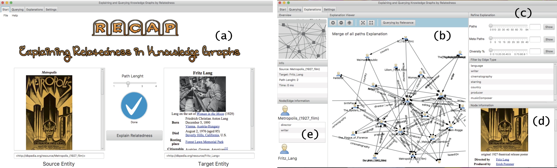
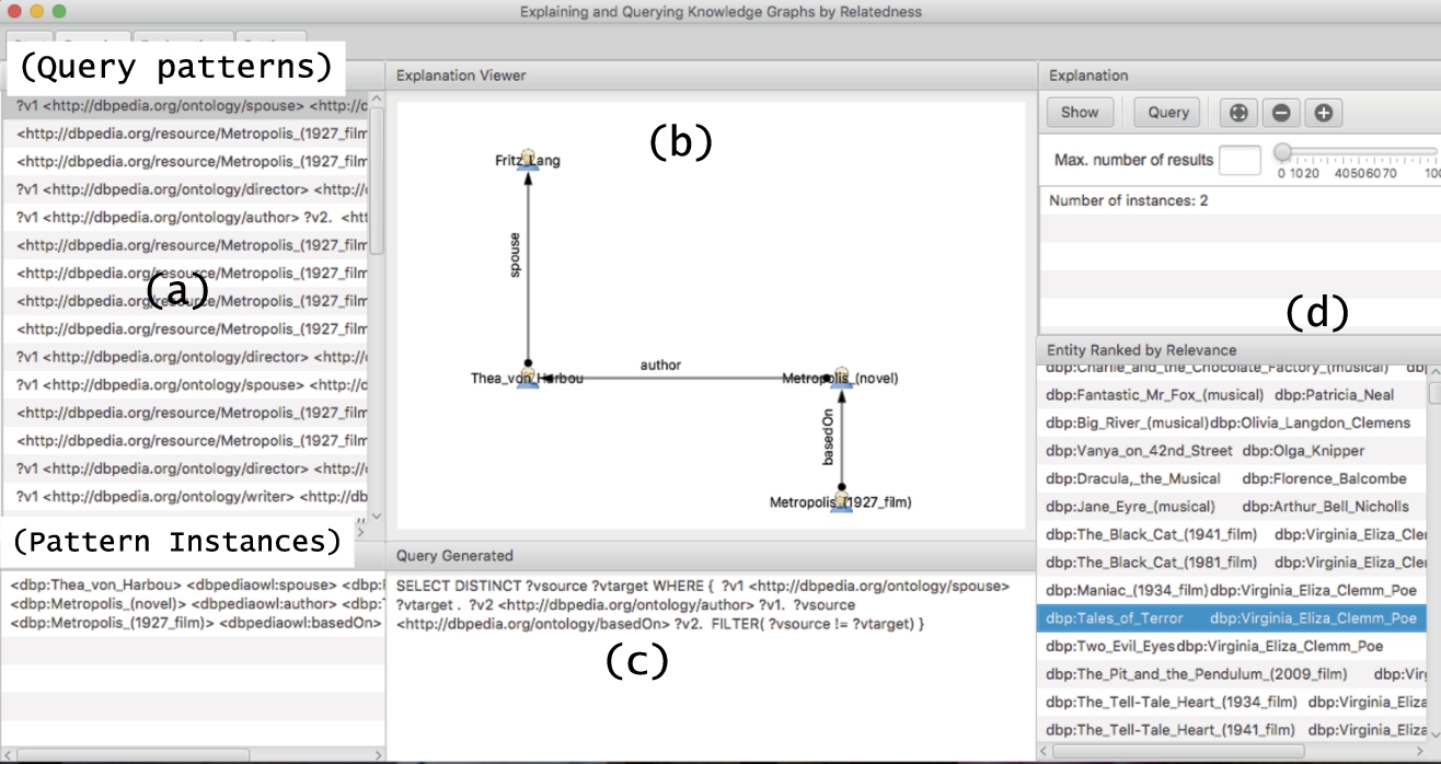
The Explanation Builder takes a set of paths either from E4D or E4S and ranks them according to the input method chosen by the user. Paths are then merged to build an explanation, which is passed to the RECAP GUI. Fig. 13(a) shows the main GUI of the tool. The user can specify the pair of input entities and get a short description. Figure 13(b) shows the part of the GUI that deals with explanations. It is possible to select different kinds of explanations (Fig. 13(c)), and obtain a description of each entity (Fig. 13(d)) and edge (Fig. 13(e)) in the explanation graph. RECAP goes beyond related approaches (e.g., REX [13], Explass [10]) that provide visual information about connectivity as it allows to build different types of explanations (e.g., graphs, sets of paths), thus controlling the amount of information visualized. RECAP has the advantage of not requiring data preprocessing; information is obtained by querying SPARQL endpoints.

Fig. 14.

An overview of the query answering algorithm.

6.2. Querying knowledge graphs by relatedness

As a concrete application scenario, we now describe how explanations can support query answering in KGs. An explanation $\mathit{E}=⟨{\mathit{w}}_{\mathit{s}}\mathrm{,}{\mathit{w}}_{\mathit{t}}\mathrm{,}{\mathit{G}}_{\mathit{e}}⟩$ can be seen as a graph including paths that link a source and target entity. The idea is to turn an explanation graph ${\mathit{G}}_{\mathit{e}}$ for an entity pair $\mathrm{(}{\mathit{w}}_{\mathit{s}}\mathrm{,}{\mathit{w}}_{\mathit{t}}\mathrm{)}$ into a query pattern, which will possibly allow retrieving other entities.

Fig. 15.

Querying knowledge graphs using relatedness explanations. Path patterns (a), explanation (b), SPARQL query (c), and suggested entities (d) ranked by popularity (PageRank [36] in this case).

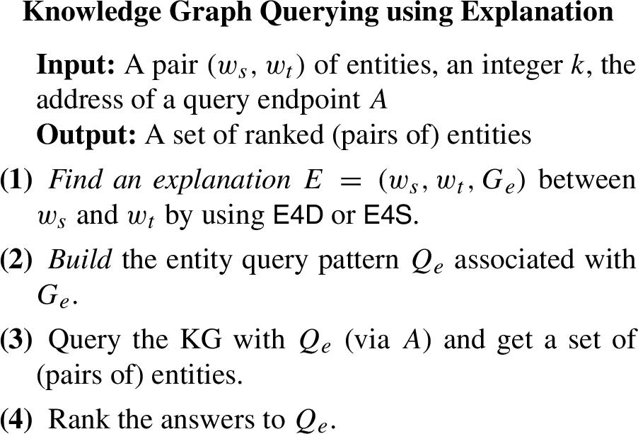
Figure 14 summarized our approach for querying KGs using relatedness explanations. We now describe steps (2) and (3) that allow to obtain the entity query pattern ${\mathit{Q}}_{\mathit{e}}$ from an explanation graph ${\mathit{G}}_{\mathit{e}}$ and, from it, a set of entity pairs. Step (4) is described in Section 6.2.1.

Definition 19 (Query Pattern).

Let $\mathit{E}=⟨{\mathit{w}}_{\mathit{s}}\mathrm{,}{\mathit{w}}_{\mathit{t}}\mathrm{,}{\mathit{G}}_{\mathit{e}}⟩$ be a relatedness explanation with ${\mathit{G}}_{\mathit{e}}=\mathrm{(}{\mathit{V}}^{\mathit{e}}\mathrm{,}{\mathcal{E}}^{\mathit{e}}\mathrm{,}{\mathit{T}}^{\mathit{e}}\mathrm{)}$ . Let ${\mathit{f}}_{\mathit{n}}:{\mathit{V}}^{\mathit{e}}\to \mathcal{V}$ a function such that ${\mathit{f}}_{\mathit{n}}\mathrm{(}{\mathit{v}}_{\mathit{i}}\mathrm{)}=?{\mathit{v}}_{\mathit{i}}$ where $\mathcal{V}$ is a set of variables. A query pattern is a tuple $\bar{\mathit{E}}=⟨?{\mathit{w}}_{\mathit{s}}\mathrm{,}?{\mathit{w}}_{\mathit{t}}\mathrm{,}{\mathit{G}}_{\mathit{e}}^{\mathit{v}}⟩$ where $?{\mathit{w}}_{\mathit{s}}\mathrm{,}?{\mathit{w}}_{\mathit{t}}\in \mathcal{V}$ and ${\mathit{G}}_{\mathit{e}}^{\mathit{v}}=\mathrm{(}{\mathit{V}}^{\mathit{v}}\mathrm{,}\mathcal{E}\mathrm{,}{\mathit{T}}^{\mathit{v}}\mathrm{)}$ with ${\mathit{V}}^{\mathit{v}}=\{{\mathit{f}}_{\mathit{n}}\mathrm{(}{\mathit{v}}_{\mathit{i}}\mathrm{)}\mathrm{,}\forall {\mathit{v}}_{\mathit{i}}\in {\mathit{V}}^{\mathit{e}}\}$ and ${\mathit{T}}^{\mathit{v}}=\{\mathrm{(}{\mathit{f}}_{\mathit{n}}\mathrm{(}{\mathit{s}}_{\mathit{i}}\mathrm{)}\mathrm{,}{\mathit{p}}_{\mathit{i}}\mathrm{,}{\mathit{f}}_{\mathit{n}}\mathrm{(}{\mathit{o}}_{\mathit{i}}\mathrm{)}\mathrm{)}\mathrm{,}\forall \mathrm{(}{\mathit{s}}_{\mathit{i}}\mathrm{,}{\mathit{p}}_{\mathit{i}}\mathrm{,}{\mathit{o}}_{\mathit{i}}\mathrm{)}\in {\mathit{T}}^{\mathit{e}}\}$

${\mathit{G}}_{\mathit{e}}^{\mathit{v}}$ is the query graph obtained by replacing all nodes in ${\mathit{G}}_{\mathit{e}}$ with query variables. Basically, a query pattern generalizes the structure of an explanation by keeping edge labels only. Query patterns are used to generate entity query patterns.

Definition 20 (Entity Query Pattern).

An entity query pattern ${\mathit{Q}}_{\mathit{e}}$ , given the query pattern $\bar{\mathit{E}}=⟨?{\mathit{w}}_{\mathit{s}}\mathrm{,}?{\mathit{w}}_{\mathit{t}}\mathrm{,}{\mathit{G}}_{\mathit{e}}^{\mathit{v}}⟩$ with ${\mathit{G}}_{\mathit{e}}^{\mathit{v}}=\mathrm{(}{\mathit{V}}^{\mathit{v}}\mathrm{,}\mathcal{E}\mathrm{,}{\mathit{T}}^{\mathit{v}}\mathrm{)}$ and ${\mathit{t}}_{\mathit{i}}\in {\mathit{T}}^{\mathit{v}}$ , $\mathit{i}\in [1\mathrm{,}\mathit{k}]$ , is a SPARQL query of the form:

In the above definition, ${\mathit{t}}_1\mathrm{,}\dots {\mathit{t}}_{\mathit{k}}$ are triple patterns and . denotes the join operator; moreover, the variables $?{\mathit{w}}_{\mathit{s}}$ and $?{\mathit{w}}_{\mathit{t}}$ are used in lieu of the entities in input. Note that query patterns are automatically derived from explanations; our approach neither requires familiarity with SPARQL nor with the underlying data/schema. The evaluation of a query pattern returns a set of pairs of entities sharing the same relatedness perspective as the input pair.

6.2.1. Ranking of results

As the number of results of ${\mathit{Q}}_{\mathit{e}}$ can be large, we describe an approach for ranking results. The problem of ranking results of SPARQL queries has been already studied (e.g., [4,31]) and is not the main purpose of the present paper. Inspired by the Google KG, we consider a simple result ranking mechanism based on the popularity of entities; specifically, we leverage the PageRank [36] algorithm. Given a pair of entities $\mathrm{(}{\mathit{w}}_1\mathrm{,}{\mathit{w}}_2\mathrm{)}$ returned when evaluating ${\mathit{Q}}_{\mathit{e}}$ , we estimate their popularity as $\mathrm{(}PR\mathrm{(}{\mathit{w}}_1\mathrm{)}+PR\mathrm{(}{\mathit{w}}_2\mathrm{)}\mathrm{)}\mathrm{/}2$ , where $PR\mathrm{(}{\mathit{w}}_{\mathit{i}}\mathrm{)}$ is the PageRank value of the entity i.

Figure 15 shows the GUI that handles querying answering using relatedness explanations. In particular, Fig. 15(a) shows path patterns (see Definition 12) while Fig. 15(b) shows the instantiation of the pattern selected. We can see that T. von Harbou was married to F. Lang and she wrote the novel Metropolis on which the film Metropolis was based. Figure 15(c) shows the automatically generated SPARQL query (see Definition 20). The underlying idea of our approach is to look for other pairs of entities that share a similar relatedness perspective. In other words, are there other pairs besides (Metropolis, F. Lang) for which there exists a spouse that wrote a novel that inspired a film? Fig. 15(d) shows some entity pairs that share this relatedness perspective. As an example, the pair (Tales of Terror, V. E. C. Poe) shares the perspective since the movie Tales of Terror was based on the novel Tales of Terror written by E. A. Poe with whom V. E. Clemm Poe was married. Ditto for the pair (The Black Cat, V. E. Clemm Poe).

7. Evaluation

We describe an experimental evaluation of our explanation framework having the following main goals:

1. Investigate the performance and scalability of E4D, our knowledge-graph-agnostic approach for building explanations, which allows to: (i) use any SPARQL-enabled KG as a source of background knowledge; (ii) avoid to set up complex processing infrastructures (in terms of data storage and computing power); (iii) work with fresh data without having to replicate and keep them up to date locally.

2. Compare E4D, which builds explanations directly by looking at paths in the data with E4S, which starts from candidate explanation patterns found in the KG schema. This will allow to understand the trade-off between working with all paths (found by E4D) and performing a later refinement and selecting explanations patterns that are of interest beforehand and then verify only those in the data (via E4S).

3. Investigate the usability of the RECAP tool as compare to related tools. This allows to have an account for its practical usability.

We describe the datasets and experimental settings in Section 7.1. Then, in Section 7.2 we report on G1. We discuss G2 in Section 7.3 and Section 7.4. Finally, G3 is dealt with in Section 7.6.

7.1. Datasets and experimental setting

There is no standard benchmark for evaluating relatedness explanation algorithms and tools. Nevertheless, some query-sets have been defined to evaluate the discovering of semantic associations, that is, paths between an entity pair. We considered a dataset of 74 entity pairs,5

⁵

Reported in Appendix B.

by extending a dataset of 24 pairs defined by Cheng et al. [10]. The dataset covers a fair large number of knowledge domains (i.e., entertainment, sport, movies, companies) and thus can give insights about the performance of our approach in different scenarios. Table 3 summarizes the algorithmic parameters used in the experiments. Note that $\mathit{k}⩽\mathit{i}$ , $\mathit{i}\in [1\mathrm{,}3]$ means that in the same run we consider paths of length up to i. As we will discuss in Section 7.6, paths of length $\mathit{k}\mathrm{>}3$ provide little insight on the relatedness of the input pair as there is a very large number of paths that involve intermediate nodes and edges that have very little in common. All the experiments were performed on a MacBook Pro with a 2.8 GHz i7 CPU and 16 GBs RAM. Results are the average of 3 runs with queries executed in random order.

Table 3

Algorithm parameters and their values

Parameter	Value	Meaning
k	1–3	Max. path length
m	5	Top-m most informative paths
p	5	Top-q related predicates used in E4S
r	0.5	Diversity range

7.1.1. Knowledge graphs used

We evaluated our explanation building algorithms by considering two different knowledge graphs (summarized in Table 4). Table 4 also reports the address of the remote SPARQL endpoint used to access the KGs. The first KG is DBpedia, which includes more than 400 million triples6

⁶

This number has been obtained by submitting a SPARQL count query to the endpoint.

while the second one is Wikidata, which includes more than 5 billion triples.⁶

We decided to use online available endpoints to have an account of how the system works in a real-world scenario. On one hand, this allows to benefit from computational resources made available by the data provider and does not require any maintenance (e.g., data update). On the other hand, this choice brings the cost of network delays, a possible load of the endpoint, and does not allow to pre-filterer data used to build explanations (e.g., by excluding literals that do not play any role in building explanations). A more comprehensive discussion about this and other design choices is available in Section 7.5.

Table 4

Knowledge graphs used in the evaluation

KG	#triples	Query Endpoint (A)
DBpedia	∼438 M	http://dbpedia.org/sparql
Wikidata	∼5 B	http://query.wikidata.org/sparql

Fig. 16.

E4D: time to find paths of increasing length in DBpedia and Wikidata.

Fig. 17.

E4D: number of paths of increasing length in DBpedia and Wikidata.

7.2. E4D: Finding explanations from the data

We start our analysis of the performance of E4D by looking at the running times of finding paths of increasing length.

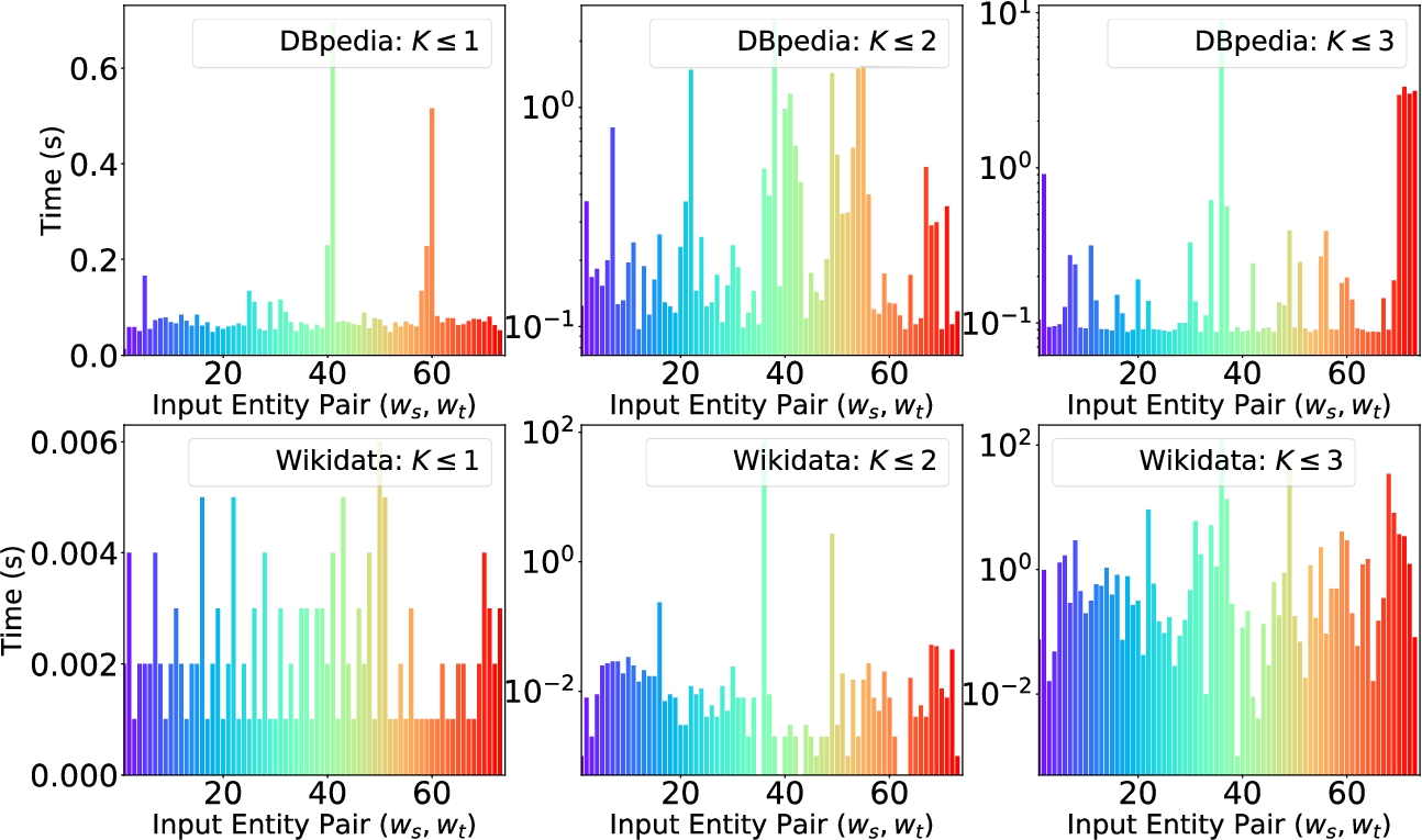
7.2.1. E4D: Running time

Figure 16 shows the running times of E4D (the mean and variance are shown in Table 5) while Fig. 17 plots the number of paths found for different values of k. Recall that for each k our algorithm retrieves paths of length up to k. In the figures, each input pair (x-axis) is identified by a different color.

Table 5

Mean and variance of running times (secs)

Distance	DBpedia		Wikidata
	Mean	Variance	Mean	Variance
$\mathit{k}⩽1$	0.09	0.009	0.002	1.558e−06
$\mathit{k}⩽2$	0.347	0.181	1.040	71.679
$\mathit{k}⩽3$	0.436	1.422	3.803	220.890

Fig. 18.

Size of ${\mathit{E}}^{\cup }$ explanations in DBpedia and Wikidata consisting in the merge of all paths found by E4D.

For $\mathit{k}⩽1$ the running time is below one second on both DBpedia and Wikidata. However, we can note in Fig. 17 that only ∼1/3 of the input pairs have at least a path of length 1 (i.e., a direct link). For $\mathit{k}⩽2$ , on DBpedia, we can see that the number of paths stays in the order of tens for most pairs with a few pairs having a relatively large number of paths (e.g., pair 38, that is, (France, Paris)). On Wikidata the number of paths is almost an order of magnitude larger with some pairs (again pair 38) having a very large number of paths. By comparing DBpedia and Wikidata we observe a similar trend, although translated in terms of absolute numbers since in the Wikidata KG most pairs have a large number of paths interlink them. The running time stays in the order of a second on both DBpedia and Wikidata with a few pairs requiring a longer time. In particular, the pair (France, Paris) is somehow a corner case; it is reasonable to have a very large number of paths between the very general entities France and Paris.

However, we believe that relatedness explanations are much more interesting for other kinds of, less obviously related, input pairs like pair 74 (C. Manson, Beach Boys). For $\mathit{k}⩽3$ , we notice the same relation between running times and the number of paths both on DBpedia and Wikidata. In the case of the latter, running times are now in the order of ten seconds (excluding some outliers). This time the number of paths is in the order of hundreds for most pairs with a larger number of entities having thousands of paths; in Wikidata the number of paths is in general much larger. This comes as no surprise due to the different sizes of the KGs, counting ∼0.5 M and ∼5 B of triples, respectively. It is also interesting to observe that pairs like (S. Spielberg, M. Report) and (York, M. Prescott), for instance, were linked by a larger number of paths in DBpedia than Wikidata, despite the much larger size of this latter KG. The aim of relatedness explanations is to provide concise (visual) graphs that can shed light about why the two entities are connected. Therefore, in what follows we investigate the size of explanations.

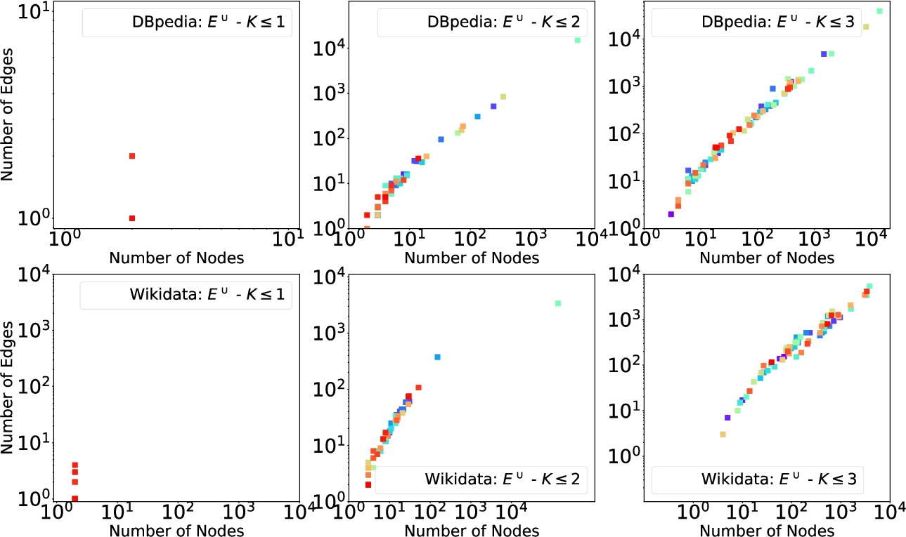
7.2.2. E4D: Explanation size

Figure 18 shows the explanation size in terms of number of unique nodes and all edges. Explanations considered are built by merging all paths and are referred to as ${\mathit{E}}^{\cup }$ (see Table 2). We can notice that for $\mathit{k}⩽1$ , there are a few available explanations, having 2 nodes and between 2 and 4 edges. These numbers are consistent in both DBpedia and Wikidata. On DBpedia, for $\mathit{k}⩽2$ , most explanations have around 10 nodes with a few exceptions where the number of nodes can be in the order of a hundred. On Wikidata, the cluster is centered between 10 and 100 nodes with a few having more than 1000 nodes. For $\mathit{k}⩽3$ explanations have a larger size variety on both DBpedia and Wikidata.

We can notice that quite many explanations have a number of nodes and edges is in the order of hundreds. Note that now the distribution is more shifted toward higher numbers, especially on Wikidata where the majority of explanations have between 200 and 600 nodes and between 100 and 1000 edges. We want to stress the fact that already for $\mathit{k}⩽3$ , most explanations become very large. This analysis suggests that considering larger values of k can even worsen the situation. Moreover, considering explanations build by the merge of all paths may hinder the understandability of a (visual) explanation already for $\mathit{k}⩽3$ . Therefore, having the possibility to control the amount of information to put into an explanation becomes crucial. Our path ranking strategies specifically deal with this aspect.

7.2.3. Refining explanations

We now discuss explanations built by considering a subset of paths interlinking an entity pair. In terms of running time, explanations based on path informativeness ${\mathit{E}}_{\mathit{m}}^{\mathit{\xi }}$ (we discuss the case $\mathit{m}=5$ ) require to compute pfitf scores; our approach computes these scores in parallel and can leverage the merge of all paths as the underlying graph (see Definition 13) thus not requiring to perform any remote query. Explanations based on pattern informativeness ${\mathit{E}}_{\mathit{m}}^{\bar{\mathit{\xi }}}$ (we discuss the case $\mathit{m}=5$ ) are less expensive since they do not analyze the informativeness of all edges in a path. Again, to count the instances satisfying a path we can use the merge of all paths as reference graph (see Definition 17). Building these kinds of explanations had a minor impact (i.e., between 0.3 and 1 seconds) on the overall running time. We do not report times since they are almost the same as those already discussed.

What changes is the size of explanations built by considering a subset of paths only. Indeed, ${\mathit{E}}_5^{\mathit{\xi }}$ , based on path informativeness, are much smaller; the typical size is ∼8 nodes and ∼10 edges on DBpedia and ∼15 nodes and ∼20 edges on Wikidata, when $\mathit{k}⩽2$ . On the other hand, ${\mathit{E}}_5^{\bar{\mathit{\xi }}}$ , based on path pattern instance, have variable size as it depends on the number of paths for each of the top-5 most informative patterns. In general, these are bigger than ${\mathit{E}}_5^{\mathit{\xi }}$ explanations (∼15 nodes and ∼20 edges on DBpedia and ∼20 nodes and ∼25 edges on Wikidata). Note that ${\mathit{E}}_5^{\bar{\mathit{\xi }}}$ explanations enable to focus on specific aspects as they include all the instantiations of each of the top-5 most informative path patterns. We will return on this aspect in Section 7.3.2 when discussing E4S, which allows choosing patterns before finding paths instead of emerging and selecting them after discovering paths as done by E4D.

We now discuss explanations built by using a diversity criterion, that is, ${\mathit{E}}^{\mathit{\delta }}$ ; these explanations are a bit more expensive in terms of running time (between 1 and 3 seconds) since they require the computation of distances between paths, even if this task leverages a multithreading approach. In terms of size, these explanations are in the same order of magnitude as ${\mathit{E}}_5^{\bar{\mathit{\xi }}}$ on DBpedia, while being a bit larger in Wikidata. We hypothesize that this behavior is due to a larger number of predicates present in Wikidata, which allows to consider a higher number of paths with the same δ value than in DBpedia. The important point of ${\mathit{E}}^{\mathit{\delta }}$ explanations is that they guarantee to also include rare edges potentially discarded by path or pattern informativeness. We also looked into explanations combining (top-5) path/pattern informativeness and diversity ( $\mathit{r}=25\mathrm{\%}$ ). In this case, the typical size is ∼20 nodes and ∼25 edges in DBpedia and a bit larger in Wikidata. The flexibility of our explanation framework, which allows to decide the amount of information to be included into an explanation, is crucial toward understanding relatedness between entities.

Fig. 19.

E4S: number of queries generated to verify candidate explanation patterns for each input pair.

Fig. 20.

Running times of E4S when considering all queries (top) and the top-5 most related to the seed predicate (bottom).

7.3. E4S: Explanations from the schema

We now discuss the E4S algorithm, which makes use of the KG schema. Recall that differently from E4D, E4S allows to build explanations about a specific relatedness perspective by giving as input both a pair of entities and a predicate. For the experiments, we took the latest version of the DBpedia ontology7

⁷

http://downloads.dbpedia.org/2014/dbpedia_2014.owl.bz2

and considered statements about rdf:type, rdfs:subClassOf, rdfs:subPropertyOf rdfs:domain and rdfs:range only. In fact, these are at the core of the notion of schema graph (see Definition 2), which is used by E4S to generate candidate explanation patterns. These pieces of schema information are also available in other KGs like Wikidata (under a different naming) and Yago, among others. In order to generate candidate explanation patterns in DBpedia, the first step of E4S is to identify domain-specific predicates. With RECAP the user can select one or more predicates for a domain. However, to run the experiments we automatized the identification of seed predicates. For each input pair, we took the top-6 most informative predicates (see Definition 14) common to the source and target entity; when there were no predicates in common, we took the top-3 most informative predicates from the source and target entity, respectively.

We ran Algorithm 1 by using each of the 6 seed predicates as input and obtained an overall set of candidate explanation patterns; from these, we obtained a set of SPARQL queries used to verify such patterns (see Section 4.3.1). Figure 19 shows the number of SPARQL queries generated for each input pair. We observe that the number of queries varies from pair to pair and can reach the order of thousands when $\mathit{k}\mathrm{>}1$ . These queries contain predicates that are related to the seed predicate in the “middle” position of triple patterns. In contrast, with E4D we have a fixed number of $2^{\mathit{k}}$ queries containing variables in the predicate position of triple patterns. The peculiarity of E4S is that it allows to reduce the number of candidates queries by focusing on those that are interesting before verifying them in the data; interestingness can be defined according to e.g., informativeness and/or diversity. In what follows we investigate this aspect.

7.3.1. E4S: Running time

We now report the running time of E4S in two different settings: (i) when considering all queries shown in Fig. 19; (ii) when only considering the top-5 queries having the highest semantic relatedness wrt the seed predicate. Running times are shown in Fig. 20. We can notice that running times when considering all queries are larger than those obtained by E4D. This comes as no surprise since the number of queries is much larger in this case. Nevertheless, getting reasonably (and visually) understandable explanations from E4D requires to apply some posterior filtering criterion like considering top-k paths, patterns, or applying a diversity criterion. Hence, the final cost of building explanations via E4D should also consider the cost of the refinement. On the other hand, E4S allows to decide a filtering criterion beforehand, thus drastically reducing the number of queries that have to be verified. To further investigate this aspect, we ran additional experiments by verifying only the top-5 queries. In particular, we start the verification from the query most semantically related wrt the target predicate and proceed with the verification until 5 queries are verified (i.e., returned some path). Running times, in this case, are reported in the bottom part of Fig. 20. As an example, for $\mathit{k}⩽3$ , running times now never exceed ten seconds. Filtering the queries to be verified introduces a significant reduction of the running times of E4S, bringing the values to be compatible with those of E4D. Nevertheless, recall that E4D still requires some pruning in order to produce (visually) understandable explanations while those produced by E4S (when applying query filtering) potentially contain fewer nodes and edges as these are built considering specific predicates. We investigate this aspect in the next section.

Fig. 21.

E4S: explanation size on DBpedia for the top-5 most related queries.

7.3.2. E4S: Explanation size

Figure 21 reports the size of explanations found by E4S when considering the verification of the top-5 most semantically related queries to the seed predicate. We note that these explanations contain a few edges while the number of nodes can be a bit larger (when $\mathit{k}⩽3$ ). It is interesting to compare the explanation sizes with those found by E4D (reported in Fig. 18). The size reduction is clear; for instance, when $\mathit{k}⩽2$ the number of nodes is around 10 for E4S while it can be up to thousand for E4D. This difference is more evident when $\mathit{k}⩽3$ where we have that the number of nodes for E4D can be much larger. We note that explanations found by E4S (when filtering the queries) contain a subset of all nodes and edges that can be found when considering all paths (as done by the merge of all paths via E4D or evaluating all queries generated by E4S). The main point of E4S is exactly to allow the generation of focused explanations, that is, explanations whose filtering criterion has been decided a priori and that can be directly (visually) “parsed” by the user.

Fig. 22.

Values of informativeness of the most informative path discovered by E4D and E4S for $\mathit{k}⩽3$ .

7.4. Comparing E4D and E4S

We now provide a more direct comparison between E4D and E4S. Although both algorithms face the problem of building relatedness explanations, they adopt two different strategies, each with its own peculiarities. E4D, which builds explanations by looking at all paths between an input pair, is useful when one wants to look at all possible ways in which the pair is interlinked. This, in some sense, allows to build general explanations where previously unknown and unexpected interesting facts can emerge. On the other hand, E4S is useful when one is interested in finding explanations focused on a certain relatedness perspective, which is expressed via the target predicate and its top-k most related predicates. One could also construct the connectivity pattern queries used by E4D (see Definition 7) with this same principle. Nevertheless, this would not allow to examine beforehand the candidate explanation patterns to perform, for instance, some filtering. Operationally, E4D explores a larger portion of the KG than that explored by E4S in order to find out interesting information. Moreover, E4S will by construction return smaller graphs thus facilitating the visual exploration, but it can miss pieces of knowledge expressed by using predicates that are semantically far from the input predicate. To have a more precise account of how the two approaches behave, we now report on an analysis of the kinds of paths found in terms of the most informative and most diverse paths.

Most Informative Path. Fig. 22 reports the values of the most informative path discovered by the two algorithms when $\mathit{k}⩽3$ . We note that there is a broad range of informativeness. As an example, for pairs like (France, Paris) the value are 0.07 and 0.05 for E4D and E4S, respectively; this value can be explained by the fact that entities in this pair are very generic in the sense that the incoming outgoing links of these and intermediate entities do not provide a high contribution in terms of informativeness (see Definition 16).

We also note that the values of informativeness given by E4D is higher than that provided by E4S. This comes as no surprise since the former algorithm considers all paths while the latter only a subset of them. By further investigating the values of informativeness, we noted that the values provided by the two algorithms usually different of about 10% for most pairs, although there are other pairs for which this difference is higher (e.g., pair 27 (Last Action Hero, Terminator 2)). Despite the values reported in Fig. 22, it is difficult to compare the algorithms in terms of path informativeness since this value does not have a fixed range as it depends on the nodes and edges inside the paths. To further understand the relative performance of the algorithms we investigate the values of path diversity.

Most Diverse Path. Path diversity is more abstract than informativeness; while the former depends on the variety of predicates in a path only, the latter also depends on the nodes in the path in terms of their incoming and outgoing edges. Differently from path informativeness, path diversity always falls in the interval $[0\mathrm{,}1]$ , where 0 means that all paths share the same predicates and 1 means that there is at least a pair of paths that predicate-wise are different. Figure 23 reports the highest values of path diversity when $\mathit{k}⩽3$ .

Fig. 23.

The highest value of diversity for E4D and E4S for $\mathit{k}⩽3$ .

We note that for most pairs it is possible to find a path that includes predicates not shared with any other path (i.e., the value of diversity equals to 1); this is true for both E4D and E4S. For other pairs it is not possible to find a diverse path; these are typically pairs that are linked by a low number of paths (e.g., pair 1 (C. Martínez, M. Seles) and pair 60 (D. Beckham, M. United)).

Note that in terms of diversity the fact that E4S considers a smaller number of paths did not have an impact on the task of finding the most diverse paths.

7.5. Discussion

We now discuss some design choices made.

Local vs Remote Data. One of the cornerstones of the proposal is to make available an explanation building framework that can work on top of any KG. This has the advantage of making the tool available even to whom does not have resources to build an infrastructure in terms of computing and storage power. The variety of KGs available as Linked Open Data and accessible via SPARQL endpoints offer a unique opportunity toward reaching this objective. Online endpoints allow to seamlessly use the explanation framework in a variety of domains with continuously updated data. On the other hand, a custom and local working mode would require to process, store, made available and update a KG for each of the domain of interest.

In general, RECAP can benefit from the computational resources of online SPARQL endpoints, when submitting queries to retrieve paths, in the same way as any other user (or application) that submits queries. Note that this can also bring the drawbacks of online endpoints like temporary unavailability and long running times in case of high processing load. The experiments were conducted on online endpoints with the precise purpose of testing how the system works on normal working conditions (in the sense that do not depend on the tool).

Table 6

Questions/responses: means (standard deviation)

Question	RECAP	RelFinder	Explass
Q1: Information overview	4.55 (0.65)	3.05 (0.77)	3.82 (0.75)
Q2: Easiness in finding information	4.45 (0.55)	4.05 (0.63)	3.85 (0.67)
Q3: Easiness in comparing/synthesizing info	4.62 (0.62)	3.10 (0.82)	4.06 (0.61)
Q4: Comprehensive support	4.81 (0.73)	3.42 (0.77)	4.15 (0.79)
Q5: Sufficient support to the task	4.67 (0.81)	3.28 (0.86)	4.23 (0.83
Q6: Running time	4.82 (0.48)	4.12 (0.72)	3.18 (0.52)

Schema Availability. Another aspect that needs to be clarified concerns the E4S algorithm. This algorithm assumes the KG to be endowed with a minimal schema definition including a hierarchy of classes (and properties) and domains and ranges of properties. This assumption is realistic in practice; popular KGs like DBpedia, Yago, and Wikidata feature even richer schema definitions. Another aspect concerns the completeness of the schema as it can be the case that some classes and properties are underspecified (e.g., missing domain and range). Our experiments on DBpedia suggest that for the dataset considered, which covers a quite broad number of domains the schema specification was sufficient. In general, one can refine/complete the portion of the schema that touches a particular domain of interest. Besides proceeding manually, RECAP can benefit from approaches that surface/refine a KG schema from the data or rely on other schema definitions like schema.org or Wordnet to complete underspecified aspects in the schema of the KG of interest.

7.6. Explanation building tools

We now report on a user study. The overall goal was to investigate the different functionalities of RECAP as compared to those of tools tackling similar problems. In particular, we considered RelFinder8

⁸

http://www.visualdataweb.org/relfinder/relfinder.php

and Explass9

⁹

http://ws.nju.edu.cn/explass/

that are tools publicly available. RelFinder is a tool that given a pair of entities and a value of distance d produces a (visual) graph composed of all paths up to distance d interlinking them. Explass takes the same input as RelFinder but tackles a slightly different problem; it focuses on finding the top-k ontological patterns that abstract a set of paths. We note that both Explass and RelFinder starts from the data to fulfill their goals; moreover, both of them only work on DBpedia. To test similar functionalities, we considered explanations found by the E4D algorithm and used DBpedia.

Experimental Setting. Twenty participants were assigned each six random pairs among the 26 entity pairs used to evaluate Explass and described in [10]. Participants were shown how the three systems work and asked to use each system (with no other support) to understand the relatedness between entities in an input pair. In order to collect the opinions from the participants, we followed the methodology adopted for the evaluation of Explass [10]. It was based on a set of five questions where the response to each question was given with an agreement value from 1 (minimal agreement) to 5 (maximal agreement). We added an additional question (i.e., Q6) in order to understand how users perceive the performance of the systems in terms of running times. We think that this is a relevant question since, besides the (visual) features, it is also important to understand if the time a user has to wait to get an answer is reasonable. The results of the evaluation for each question are reported in Table 6; the full text of the questions is reported in Appendix A.

Results. Question Q1 concerns aspects related to the support given by the tools in getting an overview of all relevant information. Users, in this respect, recognized that both Explass and RECAP provided a more comprehensive overview than RelFinder; indeed, Explass and RECAP, via path patterns, provide a more concise overview of all paths interlinking the input pair while RelFinder only shows (the merge of) all paths. This aspect was found particularly problematic by users that were asked to evaluate the tools on pairs like (B. Obama, J. W. Bush) and (J. Kirby, I. Man) linked by a large number of paths. As for Q2, which is about the easiness of finding information, participants rated RelFinder and RECAP better than Explass. In particular, participants found useful the RECAP functionality that provides a short description of the input entities (see Fig. 13(a)). Question Q3 is about functionalities of the tool that synthesize the results. In this case, RECAP and Explass were considered better than RelFinder. The visualization of unfiltered explanations (e.g., explanations including all paths) provided by the latter required some effort. On the other hand, Explass by default groups together paths belonging to the same pattern. One of the features appreciated was the ability of RECAP to control the amount of information visually shown. In fact, the RECAP functionalities allowing to show, for instance, the most informative path or the top-k most informative paths, allowed to cope with the visual overload of pairs of entities linked by a large number of paths. Q4–Q5 are about the support that the tools give to complete the task. In this case, Explass and RECAP offered more support than RelFinder. The main reason was the fact that this latter tool only allows to visualize a single type of explanation (all paths) while the other tools offered more features. RECAP was considered a more comprehensive solution also due to the fact that it allows to discover additional entities (via the query by relatedness functionality) that share a given relatedness perspective. Question Q6 was about running time. In this case, Explass was considered the least compelling system. The inter-annotator agreement, computed as the mean correlation between each pair of raters was of 0.85. RECAP was judged higher than the other two systems in all questions via LSD post-hoc tests ( $\mathit{p}\mathrm{<}0.05$ ).

Combining multiple KGs. Users also were asked to test the capability of RECAP in combining knowledge from DBpedia and Yago. In particular, starting from entities in DBpedia, the tool can look at owl:sameAs links to find the corresponding Yago entities. Then it can merge the explanations obtained from the two KGs. Users (∼75%) perceived the combination of multiple KGs as very useful for more comprehensive explanations. This is especially true when KGs cover the same domain with different levels of detail (DBpedia was judged more comprehensive than Yago). The combination also produces graphs of a bigger size. Indeed, the functionality of RECAP allowing to filter information to be included into an explanation was judged very useful (participants thought that the merge of paths ${\mathit{E}}^{\cup }$ was big already with $\mathit{k}=2$ ).

8. Related work

We review related work along different perspectives. Our analysis ranges from techniques to build explanations and/or similar notions to implemented tools.

8.1. Relatedness explanations

The problem of finding structures (e.g., paths, subgraphs) connecting entities has been tackled from different perspectives. Faloutsos et al. [12] consider edge-weighted graphs without labels and treat the input graph as an electrical network in which each edge represents a resistor with conductance. The sought connectivity subgraph is the one that can deliver as many units of electrical current as possible. Along the same line, Ramakrishnan et al. [41] consider multi-relational weighted graphs with weights assigned by looking at the schema (e.g., class and property specificity). To discover the subgraph connecting two entities, authors resort to the same algorithm as Faloutsos et al. [12].

Our work differs in the fact that we focus on building different kinds of explanations, by also controlling the kind and amount of information to be included, by using two different SPARQL-based algorithms; one that starts from the data (E4D) and the other that starts from the schema (E4S). Besides, we provide a visual tool (RECAP) with a concrete application of relatedness explanations for query answering.

Heim et al. [25] devised a tool called RelFinder, which given a pair of entities in DBpedia can produce a graph interlinking them. Differently, from our approach that can control the final explanation graph via path ranking and selection strategies, the graph found by RelFinder can quickly become too large to provide useful insights. Moreover, we also provide E4S and described the concrete use of explanations for query answering. REX [13] finds relationship explanations in the context of the Yahoo! search engine. It leverages (existing) ad-hoc algorithms for explanation enumeration and pruning as well as different measures of interestingness. There are some substantial differences between the work presented in this paper and REX. We make use of information-theoretic notions to prune the set of paths that will contribute to the explanation. While producing an explanation we take into account diversity, which allows to include into an explanation also “rare” edges. We adopt a knowledge-graph agnostic approach that relies on queries to a (remote) endpoint. Moreover, our E4S algorithm allows to start from the KG schema to build personalized explanations. Last but not least, we have described a concrete use of our approach for querying KGs. This is again achieved by via SPARQL queries to a (remote) endpoint. Voskarides et al. [52] focus on the problem of explaining relatedness making available short text descriptions. In particular, the problem is transformed into that of ranking sentences from documents in a corpus that is related to the knowledge graph. The approach described in this paper is entirely based on structured information and does not require the use of text corpora. Indeed, our aim is to produce a graph instead of a textual description.

A recent piece of work [51] tackles the problem of contextualizing facts. Authors propose a technique called neural fact contextualization method (NFCM) that given a target fact it is able to generate a set of related candidate facts (via a graph traversal algorithm); then, it uses recurrent neural networks to contextualize the fact based on a score assigned to the candidate facts. E4S adopts a different departure point; it abstracts the input pair to generate an explanation template that is used to generate an explanation hypothesis at the level of schema used to assemble an explanation graph according to different criteria (e.g., informativeness, diversity). On the other hand, NFCM uses an input fact to contextualize it by traversing the data graph.

8.2. Discovering semantic associations

A number of proposals have tackled the problem of finding semantic associations (paths) interlinking entities. Cheng et al. [10] describe an approach to find a flat list (top-K) of clusters and facet values for refocusing and refining the search in KGs. In particular, the approach can recommend frequent, informative, and small-overlapping patterns by leveraging ontological semantics, query context, and information theory. Our work differs in the fact that we aim at building explanations that are graph based on two different algorithms. Moreover, our path ranking strategies allows controlling the amount of information that will be part of an explanation thus helping the user in precisely understanding why a pair of entities is related. Last but not least, we described a concrete application of explanations for query answering. Tiddi et al. [47] tackle the problem of defining a cost-function that is able to detect the strongest relationship between two given entities in a supervised way. Authors frame the problem into a genetic programming setting and devise a technique that can learn such cost function by only looking at the topology of the subgraph (set of paths) connecting a pair of entities. The output of the process is a single path that best (in terms of the cost function) represents the relation between two entities. We start from the perspective of building explanations that are graphs in an unsupervised way. We offer two different algorithms with E4S staring from the KG schema thus giving high flexibility in choosing which kinds of patterns look interesting to build an explanation. We also describe a concrete use case of querying KGs by relatedness along with the RECAP visual tool.

Cheng et al. [8] describe an efficient graph search algorithm for finding associations among a tuple of entities, which prunes the search space by exploiting distances between entities computed based on a distance oracle. After finding a potentially large number of such associations, the approach performs a summarization of notable subgroups. Our approach is SPARQL based and can scale to very large graphs while their work on main memory. Their approach does not use the schema to prune/personalize the search for explanations. Nevertheless, combining our schema-based approach (E4S) with theirs is interesting. Considering a tuple of entities is also interesting.

Table 7

Comparison of RECAP with related tools

System	KG	O	F	Q	L
REX [13]	Yahoo!	Graph	No	No	Yes
RelFinder [25]	DBpedia	Graph	No	No	Yes
Explass [10]	DBpedia	Paths	Yes (only paths)	No	Yes
RECAP	Any	Graph/Paths	Yes (paths and graphs)	Yes	No

Bianchi et al. [7] focus on the problem of finding the most “interesting” semantic associations by defining a ranking function, which can take into account user preferences. The approach starts from a small sample of semantic associations that are rated by the user and then use it to iteratively learn a personalized ranking function. Our approach is based on two different algorithms (E4D and E4S) that can build relatedness explanations in the form of graphs. Moreover, we have implemented the RECAP tool as we believe that having a way to visually present explanations can help the user in better understanding explanations. Last but not least, as a concrete application of explanations we have implemented a relatedness based querying mechanism. Nevertheless, it would be interesting to integrate our tool with the rating mechanism described by the authors to drive the explanation visualization.

Anyanwu et al. [5], Kochut et al. [30] and Fionda et al. [16] tackle the problem of association discovering from a query language perspective. This work starts from a specific input pair while their work from a declarative specification (i.e., a query) the results of which are unknown before evaluation. Fionda et al. [17] focus on the problem fo finding graphs at the level of schema starting from the data. Our algorithm E4S does the reverse and focus on building data-level explanations. Other approaches (e.g., [29,32,34,48]) focus on the problem of relation discovery while we focus on building explanations that can be configured to include the desired amount of information. Finally, semantic search (e.g., [21]) tackles the problem of finding relationships between KG entities that match user keywords.

8.3. Path ranking

There is also a solid body of work about path ranking. A series of papers (e.g., [2,3]) focused on path ranking by leveraging ontological knowledge and information-theoretic techniques with heuristics. Aggarwal et al. [1] focus on ranking all the paths between any two entities by using measures like cohesiveness and specificity. Differently from our approach, these approaches focus on ranking only and not on building explanations. Moreover, we devise a general framework for explanations, two algorithms, and a tool. More recently, Cheng et al. [9] perform an empirical comparison of eight techniques to rank semantic associations. The evaluation is based on ground-truth rankings created by human experts. What emerged is that experts generally prefer small semantic associations consisting of entities having similar types. Moreover, semantic associations consisting of uniform relations and those consisting of diverse ones are both preferred. This study suggests that the capability of RECAP to control the size of an explanation (by selecting only a subset of paths) is useful as from the study it emerged that users prefer small explanations.

8.4. Comparison of RECAP with related tools

Table 7 summarizes the comparison of our approach with related tools. The comparison is carried out along the following dimensions: KG supported (KG), output (O), filtering capabilities (F), querying capabilities (Q), requirement of local data (L). RECAP differs from related systems in the following main respects: as for KG, RECAP is KG-independent; it only requires the availability of a (remote) query endpoint. Moreover, RECAP can combine information from multiple KGs (by leveraging owl:sameAs links). As for O and F, RECAP focuses on building different types of explanations in the form of graphs or (sets of) paths by leveraging informativeness (to estimate the relative importance of edges), diversity (to include rare edges) and their combinations. Moreover, RECAP is the only approach that can be used to query KGs (Q). As for L, neither does RECAP assume local availability of data nor any data preprocessing.

9. Concluding remarks and future work

We have introduced a framework to generate different types of relatedness explanations. We have described two different algorithms (E4D and E4S) along with different path ranking strategies. This gives high flexibility in controlling and selecting the preferred amount of information that a (visual) explanation should contain. Explanations are a versatile tool in many contexts, from information retrieval to clustering. This work has also been motived by the SENSE4US FP7 project, where there was the need to find explanations for groups of topics emerging from textual documents. As a concrete use case, we showed how explanations can be used for querying knowledge graphs in a query-by-example fashion. In the future, we plan to integrate a user feedback mechanism that can help in building more personalized explanations.