Forest logging: A trace-based analysis of large rule-based computations

Abstract

Abstract

Knowledge representation systems based on the well-founded semantics can offer the degree of scalability required for semantic web applications and make use of expressive semantic features such as Hilog, frame-based reasoning, and defeasibility theories. Such features can be compiled into Prolog tabling engines that have good support for indexing and memory management. However, due both to the power of the semantic features and to the declarative style typical of knowledge representation rules, the resources needed for query evaluation can be unpredictable. In such a situation, users need to understand the overall structure of a computation and examine problematic portions of it. This problem, of profiling a computation, differs from debugging and justification which address why a given answer was or wasn’t derived, and so profiling requires different techniques. In this paper we present a trace-based analysis technique called forest logging which has been used to profile large, heavily tabled computations. In forest logging, critical aspects of a tabled computation are logged; afterwards the log is loaded and analyzed. As implemented in XSB, forest logging slows down execution of practical programs by a constant factor that is often small; and logs containing tens or hundreds of millions of facts can be loaded and analyzed in minutes.

1. Introduction

Much of the literature on knowledge representation and reasoning (KRR) has been concerned with the use of expressive reasoning components such as ASP and $\mathcal{A}\mathcal{L}\mathcal{C}$ -based description logics. However, there has also been interest in basing KRR systems on weaker deductive methods that more easily offer the type of scalability needed by semantic web applications. For description logics, an example of such an approach is the $\mathcal{E}\mathcal{L}$ family [2]. For rule-based systems, examples are Flora-2 [12] and its commercial extensions: the Silk and Ergo systems,1

¹

http://silk.semwebcentral.org, http://coherentknowledgesystems.com

all of which are based on logic programming under the well-founded semantics. The Ergo system, for instance, is currently used as a KRR tool to leverage web-based textual information to reason about financial regulations and medical informatics. Silk and Ergo support features that are not common for rule-based systems, including the object-oriented syntax of F-logic [13], higher-order syntax based on Hilog [3], rule descriptors, the intermixture of defeasibility theories [20], and the use of bounded rationality through a technique called restraint [8], along with various types of quantitative reasoning.

The use of these features can lead to concise representation of knowledge, but also to unpredictability in the time and space a computation requires, even when such a computation terminates. This unpredictability especially emerges when a knowledge base is produced by a team of knowledge engineers working in a loosely coordinated manner to create rules that may depend on one another. In such situations, the question arises whether the size of a resource intensive computation is due to the sophistication of the reasoning it requires; to redundant or unoptimized rules; or to rules that are simply incorrect. The following example illustrates a case that arose during a KRR effort for the Silk project.

Example 1.1.

Over the course of several months, portions of the Cyc reasoner2 ²

http://www.cyc.com

and knowledge base were translated and compiled first into Flora-2 and then into XSB [19]. In addition, several hundred first-year college biology questions were then formulated and queried.3 ³

These questions were Advanced Placement exam questions published by the College Board Association (http://apcentral.collegeboard.com/).

The translated system was able to answer some of these questions quickly, often in less than 1 second of CPU time. Other questions took half a minute or more; while still others could not be answered because of timeouts, or because of aborts due to lack of memory. In general, a medium-sized query might take several minutes to execute.

Silk and Ergo are implemented using XSB [19], so that their operational semantics ultimately is based on tabled logic programming. In fact, because of the use of frames, defeasibility and Hilog, user predicates in Flora-2 and its extensions are tabled unless they are explicitly declared otherwise – a default that is the exact opposite of tabling in Prolog. To investigate the time and space required for queries like those of Example 1, a knowledge engineer who understood the operational semantics of Silk would use information about the tables to help determine why a computation was costly. For instance, she might want to examine which tabled subgoals were queried most often; how the answers were distributed among the tables; how the queries depended on one another; and how those dependencies affected the overall search. These questions indicate a need to model a tabled evaluation as a structure that can be examined in itself. Accordingly, we denote the problem of exploring large tabled computations as the Profiling Problem. Note that profiling addresses the nature of a computation as a whole in order to determine why a computation may not terminate, or why it is costly if it does terminate. Profiling may thus be used on correctly executing programs, and does not address the question of why given solutions are returned or omitted. For this reason, profiling differs from previously reported approaches based on procedural or declarative debugging or on justification (e.g., [9,16]).

This paper presents forest logging, an approach to the profiling problem based on a trace-based analysis of SLG forests, an operational semantics for tabling. As its name implies, operational aspects of a computation are written to a log that is later loaded and analyzed. Specifically,

We present the design of the logs, and formalize their properties; in particular we show how logs preserve dependency information, and specify the conditions under which the logs can construct a homomorphic image of an SLG forest.

We present analysis predicates to display operational information about a tabled computation in an efficient manner, and describe how these routines can be customized in order to represent dependency and other information at different levels of abstraction.

We demonstrate by benchmark tests that the overhead of logging is a constant factor. We demonstrate the scalability of log analysis which can load and analyze logs of hundreds of millions of facts.

Section 2 informally reviews SLG and presents the format of forest logs. Some basic properties are shown in Section 3, while Section 4 discusses the analysis routines and describes the implementation of forest logging along with performance results. Related work is covered in Section 6.

Fig. 1.

A Definite Program and SLG Forest for Evaluation of the Query reach(1,Y).

All forest logging features discussed in this paper are available in the latest release of XSB (version 3.5). In addition, these features form the basis of the forest logging library in the publically available version of Flora-2 (version 0.99.3), as well as in the commercial Silk and Ergo systems.

2. Representing an SLG forest via a log

SLG resolution (Linear resolution with Selection function for General logic programs) [4] was formulated in [18], to model a tabled evaluation as a sequence of forests of SLG trees. Before discussing the logs themselves, we review those aspects of the forest of trees model for SLG that are necessary to understand forest logging and its applications. As SLG and its extensions have been presented in the literature, our review is largely an informal overview; for full coverage with formal definitions see the references contained in [19]. All code examples are in Prolog syntax.

2.1. A review of SLG by examples

For simplicity, we restrict the discussion of SLG to finitely terminating evaluations (which correspond to forests with a finite set of finite trees), and always assume a left-to-right literal selection strategy.

2.1.1. Definite programs

We begin with an example of SLG evaluation of a query to a definite program.

Example 2.1.

Figure 1 shows a simple program along with an SLG forest for the query reach(1,Y) to the right-recursive tabled predicate reach/2. An SLG forest consists of an SLG tree associated with each tabled subgoal S (where variant subgoals are considered to be identical); each such tree has root $\mathit{S}\text{:-}|\mathit{S}$ . Each SLG operation transforms a given forest ${\mathcal{F}}_{\mathit{n}}$ to a new forest ${\mathcal{F}}_{\mathit{n}+1}$ by adding a new tree, adding a new node, or by annotating a tree. As a result, each SLG tree represents the resolution steps that have been executed to derive answers for its root subgoal S.

Given an SLG tree $\mathcal{T}$ with root $\mathit{S}\text{:-}|\mathit{S}$ , $\mathcal{T}$ is sometimes referred to as the tree for S. In general, nodes of an SLG tree for S have the form $\mathrm{(}\mathit{S}\text{:-}\mathit{Delays}|\mathit{Goals}\mathrm{)}\mathit{\theta }$ ; where Goals is the sequence of literals remaining to prove $\mathit{S}\mathit{\theta }$ ; Delays are used for negation and are explained below, as are the numbers associated with each node. Children of a root node are obtained through resolution against program clauses, modeled in SLG by the operation program clause resolution. Children of non-root nodes are obtained through the SLG answer resolution operation if the (left most) selected literal is tabled (e.g., children of the node reach(1,Y):-|reach(2,Y));4 ⁴

We slightly abuse terminology since it is the predicate symbol of the atom within the literal that is tabled. We further abuse terminology by sometimes using selected literal to refer to the underlying atom on which the literal is based, when it is clear to do so.

or via program clause resolution if the leftmost selected literal is not tabled (e.g., children of the node reach(1,Y):-|edge(1,Z),reach(Z,Y)). Nodes with empty Goals are termed answers.

The evaluation keeps track of each tabled subgoal S’ that it encounters by creating a tree for S’ via the new subgoal operation. Later if S’ is selected again, resolution will use answers from the tree for S’ rather than program clauses; if no answers for S’ are available, the computation will suspend and try to derive answers using some other computation path. Once additional answers have been derived, the evaluation will resume the suspended computation. Similarly, after a computation has resolved all answers currently available for S’, the computation path will suspend, and resume after further answers are found.5 ⁵

This explanation implicitly assumes call variance: that a new tree is created for S’ if there is not already a tree for (a variant of) S’.

When it is determined that a (perhaps singleton) set $\mathcal{S}$ of subgoals can produce no more answers, the tree for every subgoal in $\mathcal{S}$ is marked as completed (cf. the tree for reach(2,Y) in Fig. 1). The incremental use of completion within tabling is a critical feature to supporting the well-founded semantics as it causes most atoms in unfounded sets to be set to false: in fact the use of completion is sufficient to correctly evaluate unfounded sets in definite programs. From an implementational point of view, stack space and other resources for a completed subgoal ${\mathit{S}}_{\mathit{comp}}$ can be reclaimed – apart from the table for ${\mathit{S}}_{\mathit{comp}}$ consisting of ${\mathit{S}}_{\mathit{comp}}$ and its answers.

As seen from Example 2.1, a tabled evaluation evaluates mutually dependent sets of subgoals, marking them as completed when it is no longer possible to derive answers for these subgoals. In this way, a tabled evaluation can be viewed as a series of fixed point computations for sets of interdependent subgoals. Because of these considerations, much of the operational state of a SLG forest $\mathcal{F}$ can be captured by a Subgoal Dependency Graph.

Definition 2.1 (Subgoal Dependency Graph (SDG)).

Let $\mathcal{F}$ be a forest, and let ${\mathit{S}}_1\text{:-}|{\mathit{S}}_1$ be the root of a non-completed tree in $\mathcal{F}$ . The subgoal ${\mathit{S}}_1$ directly depends on a subgoal ${\mathit{S}}_2$ iff ${\mathit{S}}_2$ is not completed in $\mathcal{F}$ , and there is some node N in the tree for ${\mathit{S}}_1$ such that ${\mathit{S}}_2$ is the underlying subgoal of the selected literal of N.

The Subgoal Dependency Graph of $\mathcal{F}$ $\mathit{SDG}\mathrm{(}\mathcal{F}\mathrm{)}=\mathrm{(}\mathit{V}\mathrm{,}\mathit{E}\mathrm{)}$ of $\mathcal{F}$ is a directed graph in which $\mathrm{(}{\mathit{S}}_{\mathit{i}}\mathrm{,}{\mathit{S}}_{\mathit{j}}\mathrm{)}\in \mathit{E}$ iff subgoal ${\mathit{S}}_{\mathit{i}}$ directly depends on subgoal ${\mathit{S}}_{\mathit{j}}$ , and V is the underlying set of nodes in E. ${\mathit{S}}_1$ “depends on” ${\mathit{S}}_2$ in $\mathcal{F}$ if there is a path from ${\mathit{S}}_1$ to ${\mathit{S}}_2$ in $\mathit{SDG}\mathrm{(}\mathcal{F}\mathrm{)}$ .

Since $\mathit{SDG}\mathrm{(}\mathcal{F}\mathrm{)}$ is a directed graph, sets of subgoals that are mutually recursive in $\mathcal{F}$ can be captured as Strongly Connected Components (SCCs) of $\mathit{SDG}\mathrm{(}\mathcal{F}\mathrm{)}$ . In Fig. 1, there is a single SCC consisting of reach(1,Y) and reach(3,Y), as reach(2,Y) is completed. While SCCs are critical for determining when subgoals can be completed, if an answer for a tabled subgoal S is derived that has the empty substitution, every ground atomic fact that unifies with S is true in the model of the program. Accordingly, S can be completed before the other subgoals in its SCC through early completion. Otherwise, a subgoal S can be completed when all possible resolution steps have been performed for S and the other subgoals in its SCC.

Understanding the changing dependencies of an evaluation is critical to a number of operational aspects. For instance, a local evaluation restricts operations so that there is always a unique maximal independent SCC. Note that an SCC $\mathcal{S}$ is independent iff no subgoal in $\mathcal{S}$ depends on any (non-completed) subgoals that is not in $\mathcal{S}$ itself, and an SCC is maximal iff it is not a subgraph of any other SCC. Local evaluation is efficient for many applications since it can be shown that it performs a “depth-first” search through SCCs. However if there are several operations possible within a maximal independent SCC, their order is not specified within a local evaluation. The number associated with each node in Fig. 1 corresponds to the node’s creation under XSB’s implementation of local evaluation (and is not part of an SLG tree per se).

2.1.2. Normal programs

Arguably, the main difference between SLG resolution and other tabling methods is the use of delaying and simplification to handle default negation.

Fig. 2.

A Normal Program ${\mathit{P}}_{\mathit{norm}}$ and SLG Forest for Evaluation of the Query p(c).

Example 2.2.

Figure 2 shows a program with negation, ${\mathit{P}}_{\mathit{norm}}$ and illustrates SLG resolution for the query p(c) to ${\mathit{P}}_{\mathit{norm}}$ . The nodes in Fig. 2 have been annotated with the order in which they were created under an instance of local evaluation; and as mentioned in Example 1, the symbol | in a node separates the unresolved goals to its right from the delayed goals to its left. In the evaluation state where nodes 1 through 11 have been created, p(b) has been completed, and in fact was early completed so that the program clause p(X):-t(X,Y,Z),not p(Y),not p(Z) did not need to be resolved against p(b). The only non-completed subgoals, p(a) and p(c), are in the same SCC. There are no more clauses or answers to resolve, but p(a) is involved in a loop through negation with itself in node 5, and nodes 2 and 11 involve p(a) and p(c) in a negative loop.

In situations such as this, where all resolution has been performed for nodes in an SCC, an evaluation may have to apply a delaying operation to a negative literal such as not p(a), in order to explore whether other literals to its right might fail. In a forest where different nodes each have a selected literal that could be delayed (e.g., in nodes 2, 5, or 11), an arbitrary node is chosen. In this case, the evaluation applys a delaying operation to the selected literal of node 11 to produce 12, whose selected literal is not p(b). Since node 8 is an answer for p(b) with empty Delays (termed an unconditional answer), a negative return operation creates node 13, termed a failure node), signifying that the computation path has failed (node 10 was produced in a similar manner). Next, a delaying operation is applied to the selected literal of node 2 to produce node 14, which is a conditional answer – an answer with a non-empty Delays set. The final delaying operation is applied to the literal not p(a) in node 5, so that the new selected literal for its child, node 15, is not p(b). As with nodes 10 and 13, a negative return operation produces the failure node, node 16.

At this stage the SCC {p(a),p(c)} is completely evaluated meaning that there are no more operations applicable for goal literals (as opposed to delay literals). Since p(a) is completely evaluated with no answers, conditional or otherwise, the evaluation determines it to be failed as part of a completion operation. Afterwards, a simplification operation can be applied to the conditional answer of node 14, removing not p(a) from its Delays. leading to the unconditional answer in node 17 and success of the literal p(c).

There is one additional SLG operation that was not used in either Example 2.1 or 2.2. The answer completion operation fails sets of conditional answers that correspond to unfounded sets by creating failure nodes as their children.6 ⁶

Failure nodes are only created by the negative return operation, to indicate that derivation of an atom A atom has failed a computation path that depends on not A, and to denote the failure of conditional answers by the action of simplification or answer completion operations [18].

Although answer completion is needed to ensure the completeness of SLG (cf. [4] for details), the operation is rarely needed in the practical strategies used by tabling engines, as most unfounded sets are detected during completion operations.

2.2. The forest log

Forest logging allows one to run a tabled query and to produce a log, from which a number of properties of the SLG forest can be inferred. The design of the log attempts to balance several goals: the log should be as informative as possible, but also easy to use and should not overly slow down computations. The log (or trace) consists of Prolog-readable facts (or events) that may be loaded and analyzed, leading to the need to support quick load times and scalable analysis routines.7

⁷

For presentation purposes we consider only tabling with call variance, and local evaluation. However the forest logging features described here are also implemented for call subsumption and for other scheduling strategies.

The log facts described below correspond directly to SLG operations, except as noted. Each log fact has a counter Cntr, indicating the ordinal number of the fact within the log. Since logs can be very large, an effort is made to keep only the most critical information in the logs so that their memory footprint is kept to a minimum.

• A call to a tabled subgoal. When a literal L is selected in a node N, where N is in the tree for ${\mathit{S}}_{\mathit{caller}}$ and L is positive ( $\mathit{L}={\mathit{S}}_{\mathit{called}}$ ) then a fact $$\mathit{t}\mathit{c}\mathrm{(}{\mathit{S}}_{\mathit{called}}\mathrm{,}{\mathit{S}}_{\mathit{caller}}\mathrm{,}\mathit{State}\mathrm{,}\mathit{Cntr}\mathrm{)}$$ is logged (“tc” stands for “tabled call”). State is

• cmp if ${\mathit{S}}_{\mathit{called}}$ is not a new subgoal and has been completed

• incmp if ${\mathit{S}}_{\mathit{called}}$ is not a new subgoal but has not been completed

If the selected literal L is negative and $\mathit{L}=\mathit{not}{\mathit{S}}_{\mathit{called}}$ , a fact $$\mathit{n}\mathit{c}\mathrm{(}{\mathit{S}}_{\mathit{called}}\mathrm{,}{\mathit{S}}_{\mathit{caller}}\mathrm{,}\mathit{State}\mathrm{,}\mathit{Cntr}\mathrm{)}$$ is logged instead (“nc” stands for “negative call”).

Note that if $\mathit{state}=\mathit{new}$ , tc/4 and nc/4 correspond to the new subgoal operation; otherwise they do not correspond to an SLG operation, but instead directly log dependency information. If ${\mathit{S}}_{\mathit{called}}$ is the first tabled subgoal called in an evaluation, then ${\mathit{S}}_{\mathit{caller}}$ is set to null.

• answer resolution. When an answer $$\mathit{A}={\mathit{S}}_{\mathit{called}}\mathit{\theta }\text{:-}\mathit{Delays}|$$ is returned to a selected positive literal ${\mathit{S}}_{\mathit{called}}$ in a tree for ${\mathit{S}}_{\mathit{caller}}$ , a fact $$\mathit{ar}\mathrm{(}\mathit{\theta }\mathrm{,}{\mathit{S}}_{\mathit{called}}\mathrm{,}{\mathit{S}}_{\mathit{caller}}\mathrm{,}\mathit{Cntr}\mathrm{)}$$ is logged if A is unconditional (i.e., if $\mathit{Delays}$ is empty); and a fact $$\mathit{dar}\mathrm{(}\mathit{\theta }\mathrm{,}{\mathit{S}}_{\mathit{called}}\mathrm{,}{\mathit{S}}_{\mathit{caller}}\mathrm{,}\mathit{Cntr}\mathrm{)}$$ is logged if A is conditional.

Although answer resolution operations are logged, program clause resolution operations are not; attempts to log these operations usually slowed down computations so much that logging became unusable for all but small computations.

negative return operations are logged in a similar manner. as answer resolution.

negative return. For a node $$\mathit{N}={\mathit{S}}_{\mathit{caller}}\mathit{\theta }\text{:-}\mathit{Delays}|\mathit{not}{\mathit{S}}_{\mathit{called}}\mathrm{,}\mathit{Body}$$ with ${\mathit{S}}_{\mathit{called}}$ a ground atom, the SLG negative return will produce a child fail for N if ${\mathit{S}}_{\mathit{called}}$ is successful, and a child $${\mathit{S}}_{\mathit{caller}}\mathit{\theta }\text{:-}\mathit{Delays}|\mathit{Body}$$ if ${\mathit{S}}_{\mathit{called}}$ is failed. In this latter case, when ${\mathit{S}}_{\mathit{called}}$ is failed (sometimes called a negative success operation), a fact $$\mathit{nr}\mathrm{(}{\mathit{S}}_{\mathit{called}}\mathrm{,}{\mathit{S}}_{\mathit{caller}}\mathrm{,}\mathit{Cntr}\mathrm{)}$$ is logged.

negative return operations are not logged when creating a failure node as a child, as the failure of a negative literal can be inferred from absence of other logged facts.

The logging of new answers does not correspond to an SLG operation but is useful for analysis.

New Answer. When a new answer $$\mathit{N}=\mathrm{(}{\mathit{Subgoal}}_{\mathit{caller}}\text{:-}\mathit{D}|\mathrm{)}\mathit{\theta }$$ is derived for subgoal ${\mathit{S}}_{\mathit{caller}}$ (i.e., N is not already an answer for ${\mathit{S}}_{\mathit{caller}}$ ) a fact $$\mathit{na}\mathrm{(}\mathit{\theta }\mathrm{,}{\mathit{S}}_{\mathit{caller}}\mathrm{,}\mathit{Cntr}\mathrm{)}$$ is logged if N is unconditional ( $\mathit{D}=\varnothing$ ) and $$\mathit{na}\mathrm{(}\mathit{\theta }\mathrm{,}{\mathit{S}}_{\mathit{caller}}\mathrm{,}\mathit{D}\mathrm{,}\mathit{Cntr}\mathrm{)}$$ is logged if Nis conditional.

Note that na/3 can be seen as a specialization of na/4 that reduces the memory footprint of the loaded log. A similar specialization is described below for simplification.

Fig. 3.

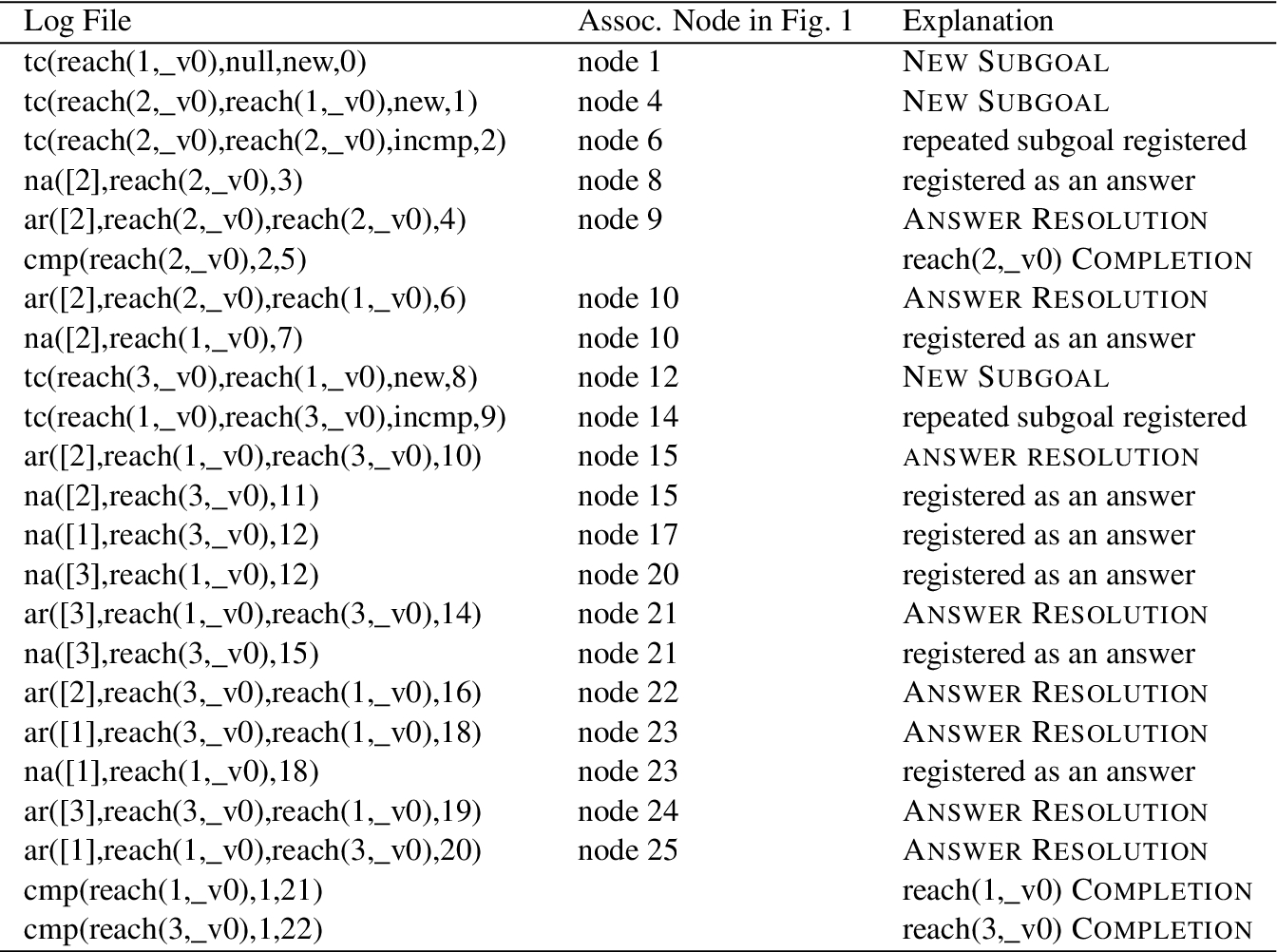
A Log File Corresponding to the SLG Forest in Fig. 1.

• completion. When an SCC $\mathcal{S}$ is completed, a fact $$\mathit{cmp}\mathrm{(}\mathit{S}\mathrm{,}{\mathit{SCC}}_{\mathit{ind}}\mathrm{,}\mathit{Cntr}\mathrm{)}$$ is logged for each $\mathit{S}\in \mathcal{S}$ . Here ${\mathit{SCC}}_{\mathit{ind}}$ is a index that groups subgoals into their mutually recursive components at the time they were completed. If S was early completed, a fact $$\mathit{cmp}\mathrm{(}\mathit{S}\mathrm{,}\mathit{ec}\mathrm{,}\mathit{Cntr}\mathrm{)}$$ is logged at the time of early completion. When the original SCC for S is completed, another completion fact for S will be logged indicating its index as just described and showing (for the purpose of analysis) the SCC in which S had been called.

• delaying When the selected literal $\mathit{not}\mathit{A}$ is delayed in a node in a tree for ${\mathit{S}}_{\mathit{caller}}$ , a fact $$\mathit{dly}\mathrm{(}\mathit{A}\mathrm{,}{\mathit{S}}_{\mathit{caller}}\mathrm{,}\mathit{Cntr}\mathrm{)}$$ is logged.

• simplification operations are logged as follows. Let ${\mathit{S}}_{\mathit{caller}}\mathit{\theta }\text{:-}\mathit{D}|$ be the answer to which simplification is applied.

• answer completion. If answer completion fails an answer ${\mathit{S}}_{\mathit{caller}}\mathit{\theta }$ in a tree for ${\mathit{S}}_{\mathit{caller}}$ , a fact $$\mathit{ansc}\mathrm{(}\mathit{\theta }\mathrm{,}{\mathit{S}}_{\mathit{caller}}\mathrm{,}\mathit{Cntr}\mathrm{)}$$ is logged.8 ⁸

  answer completion differs from simplification since it completes sets of answers corresponding to unfounded sets of atoms that have not been failed due to incremental completion.

Fig. 4.

A Log File Corresponding to the SLG Forest in Fig. 2.

Example 2.3.

The forest for reach(1,Y) in Example 2.1 has the log file as shown in Fig. 3.9 ⁹

As mentioned above, no fact is logged for an answer A to a subgoal S unless A is newly added for S. For instance, no fact is logged for the creation of the answer reach(1,2) in node 19, since the same atom was added as an answer by node 10 (and logged).

The actual log file facts are shown, along with the associated node they produced (if any) and an explanation. Similarly, the log file for the forest in Example 2.2 is shown in Fig. 4.

3. Properties of the forest log

Forest logs capture several important aspects of tabled computations. We begin by showing how they capture the subgoal dependency graph of a given forest (Definition 2.1) a property that is heavily used in Section 4. Next, Section 3.2 clarifies the extent to which a forest log can be used to reproduce an SLG forest, by discussing conditions under which a homomorphic image of an SLG forest can be constructed from a log.

3.1. Capturing dependency information

Definition 3.1.

Let $\mathcal{L}$ be a forest log with n facts, and let $0⩽\mathit{c}⩽\mathit{n}$ . Then the log dependency graph induced by c: $\mathrm{(}\mathit{V}\mathrm{,}\mathit{E}\mathrm{)}$ , is defined as follows.

A subgoal S is incomplete in $\mathcal{L}$ if $$\neg \exists {\mathcal{S}}_{\mathit{scc}}\mathrm{,}{\mathit{c}}^{″}.\mathrm{(}\mathrm{(}\mathit{cmp}\mathrm{(}\mathit{S}\mathrm{,}{\mathcal{S}}_{\mathit{scc}}\mathrm{,}{\mathit{c}}^{″}\mathrm{)}\in \mathcal{L}\text{and}{\mathit{c}}^{″}⩽\mathit{c}$$

$\mathrm{(}{\mathit{S}}_1\mathrm{,}{\mathit{S}}_2\mathrm{)}\in \mathit{E}$ for every fact $\mathit{tc}\mathrm{(}{\mathit{S}}_2\mathrm{,}{\mathit{S}}_1\mathrm{,}\mathit{state}\mathrm{,}{\mathit{c}}^{\prime }\mathrm{)}$ or $\mathit{nc}\mathrm{(}{\mathit{S}}_2\mathrm{,}{\mathit{S}}_1\mathrm{,}\mathit{state}\mathrm{,}{\mathit{c}}^{\prime }\mathrm{)}$ in $\mathcal{L}$ such that ${\mathit{c}}^{\prime }⩽\mathit{c}$ , ${\mathit{S}}_1\ne \mathit{null}$ , and ${\mathit{S}}_1\mathrm{,}{\mathit{S}}_2$ are incomplete in $\mathcal{L}$ .

V is the underlying set of nodes in E.

Since the log dependency graph is parameterized by a log’s counter, the log can be used to construct the SDG (Definition 2.1) at various stages in the evaluation. This is formalized by Theorem 3.1 which states that the SDG for any forest of an evaluation can be reconstructed from the log dependency graph. This theorem directly underlies the analysis routines of Section 4; and because it holds for any forest, the theorem also underlies analysis of partial computations – e.g., computations that were interrupted because they were suspected to be non-terminating (cf. the discussion of the Terminyzer tool [15] in Section 6).

To be able to reconstruct the SDG of a given forest $\mathcal{F}$ , there needs to be a guarantee of correspondence between the creation of $\mathcal{F}$ and the time when given facts are logged. A property termed eager subgoal logging is sufficient for this. Eager subgoal logging means that whenever a tabled literal L is selected in a tree ${\mathit{S}}_{\mathit{caller}}$ , a $\mathit{tc}\mathrm{/}4$ or $\mathit{nc}\mathrm{/}4$ fact is immediately logged, regardless of whether a new subgoal operation is applicable. For instance, if the underlying atom of the positive literal L is ${\mathit{S}}_{\mathit{called}}$ , then $$\mathit{tc}\mathrm{(}{\mathit{S}}_{\mathit{called}}\mathrm{,}{\mathit{S}}_{\mathit{caller}}\mathrm{,}⟨\mathit{state}⟩\mathrm{,}{\mathit{c}}_{\mathit{i}}+1\mathrm{)}.$$ is logged, with the value of $\mathit{state}$ as new, cmp or incmp. There is thus a difference in the behavior of the logging mechanism from the formalism of SLG, as a new subgoal operation is performed only if ${\mathit{S}}_{\mathit{called}}$ is new to the evaluation. Eager subgoal logging is supported by XSB, and should be easy to guarantee for any tabling engine that implements forest logging.10 ¹⁰

Within XSB this is done within the tabletry instruction (cf. [17]).

Theorem 3.1.

Let $\mathcal{E}={\mathcal{F}}_0\mathrm{,}\dots \mathrm{,}{\mathcal{F}}_{\mathit{n}}$ be an SLG evaluation and $\mathcal{L}$ a log created using eager subgoal logging. Then for any $\mathit{SDG}\mathrm{(}{\mathcal{F}}_{\mathit{i}}\mathrm{)}$ , $0⩽\mathit{i}⩽\mathit{n}$ , there is a c such that $\mathit{SDG}\mathrm{(}{\mathcal{F}}_{\mathit{i}}\mathrm{)}$ is isomorphic to the log dependency graph induced by c.11 ¹¹

Proofs are provided in the appendix of this paper.

3.2. Constructing a homomorphism of an SLG forest

Because SLG forests capture the operational aspects of tabling, the ability to fully reconstruct a forest would mean that a wide variety of operational properties could be obtained by analyzing a log. However, because forest logs do not keep track of program clause resolution, reconstructing a tree is not always possible. Given a forest log and program, questions then arise of how much can be reconstructed, and under what conditions. This section defines a homomorphism of SLG trees, and shows sufficient conditions under which a homomorphic image of an SLG tree can be constructed.

More precisely, forest logging may lose information about the direct edges between nodes within an SLG tree $\mathcal{T}$ if there is a significant amount of non-tabled resolution required to prove the root subgoal of $\mathcal{T}$ . We begin by characterizing a morphism that removes information about program clause resolution corresponding to cases where it may be difficult to reconstruct from a log and program.

Definition 3.2.

Let $\mathcal{T}$ be an SLG tree. The graph morphism $\mathcal{H}\mathrm{(}\mathcal{T}\mathrm{)}$ is defined as follows.

For any node $\mathit{n}\in \mathcal{T}$ , $\mathcal{H}\mathrm{(}\mathit{n}\mathrm{)}$ is defined as:

• If the selected literal of n is tabled, then $\mathcal{H}\mathrm{(}\mathit{n}\mathrm{)}=\mathit{n}$ ;

• If n is the immediate child of the root of $\mathcal{T}$ , then $\mathcal{H}\mathrm{(}\mathit{n}\mathrm{)}=\mathit{n}$ ;

• If n is an answer or failure node whose nearest ancestor either has a selected tabled literal or is in $\mathcal{H}\mathrm{(}\mathcal{T}\mathrm{)}$ , then $\mathcal{H}\mathrm{(}\mathit{n}\mathrm{)}=\mathit{n}$ ;

• Otherwise, $\mathcal{H}\mathrm{(}\mathit{n}\mathrm{)}$ is the closest ancestor of n whose selected literal is tabled.

If there is an edge between nodes ${\mathit{n}}_1$ and ${\mathit{n}}_2$ in $\mathcal{T}$ , then there is either an edge between $\mathcal{H}\mathrm{(}{\mathit{n}}_1\mathrm{)}$ and $\mathcal{H}\mathrm{(}{\mathit{n}}_2\mathrm{)}$ or $\mathcal{H}\mathrm{(}{\mathit{n}}_1\mathrm{)}=\mathcal{H}\mathrm{(}{\mathit{n}}_2\mathrm{)}$ .

Let $\mathcal{F}$ be an SLG Forest. Then $\mathcal{H}\mathrm{(}\mathcal{F}\mathrm{)}$ is defined as the union of $\mathcal{H}\mathrm{(}\mathcal{T}\mathrm{)}$ for each $\mathcal{T}\in \mathcal{F}$ .

Note that since the root of any SLG tree has a selected tabled literal, any node whose selected literal is non-tabled has an ancestor that is tabled; because the ancestor relation is a tree, the closest such node is unique, so that $\mathcal{H}$ is well-defined. Given these considerations, it is evident that $\mathcal{H}$ defines a homomorphism of an SLG forest $\mathcal{F}$ where $\mathcal{F}$ is taken as a graph with labeled nodes.

Fig. 5.

Homomorphic Image of the SLG Forest of Fig. 1.

Example 3.1.

The homomorphism of Definition 3.2 is partially illustrated by its effect on the forest of Fig. 1 as shown in Fig. 5. It can be seen that for an SLG tree $\mathcal{T}$ , the root subgoal of $\mathcal{T}$ is always in $\mathcal{H}\mathrm{(}\mathcal{T}\mathrm{)}$ by condition 1(a), and its immediate children by condition 1(b). Condition 1(c) states that an answer A will be in $\mathcal{H}\mathrm{(}\mathcal{T}\mathrm{)}$ if its immediate parent has a selected tabled literal. In the case of the forest in Fig. 1, the only nodes lost are the answers 8, 17, 19, and 20, whose parent does not have a selected tabled literal. However, note that by condition 1(c) if A is in $\mathcal{H}\mathrm{(}\mathcal{T}\mathrm{)}$ , any children of A formed by simplification or answer completion will also be in $\mathcal{H}\mathrm{(}\mathcal{T}\mathrm{)}$ .

In order to reconstruct an SLG tree in $\mathcal{T}$ from $\mathcal{H}\mathrm{(}\mathcal{T}\mathrm{)}$ , the parent of each logged fact f needs to be determined and the edges themselves constructed. When answer resolution and other tabling operations are logged, their representation of the caller and called subgoals can be used for this purpose. However in the case of program clauses resolution, the program clauses must be sufficiently distinct so that the parent of each fact can be uniquely identified. These conditions are specified by Definition 3.3. Definition 3.3.

Let $\mathit{Body}$ and ${\mathit{Body}}^{\prime }$ be two sequences of literals. Then $\mathit{Body}$ and ${\mathit{Body}}^{\prime }$ are distinguishable if

Both $\mathit{Body}$ and ${\mathit{Body}}^{\prime }$ contain at least one tabled literal, $\mathit{Body}={\mathit{L}}_1\mathrm{,}\dots \mathrm{,}{\mathit{L}}_{\mathit{n}}$ and ${\mathit{Body}}^{\prime }={\mathit{L}}_1^{\prime }\mathrm{,}\dots \mathrm{,}{\mathit{L}}_{\mathit{n}}^{\prime }$ and

1. The leftmost literals ${\mathit{L}}_1$ and ${\mathit{L}}_1^{\prime }$ are tabled and the sequences ${\mathit{L}}_2\mathrm{,}\dots \mathrm{,}{\mathit{L}}_{\mathit{n}}$ and ${\mathit{L}}_2^{\prime }\mathrm{,}\dots \mathrm{,}{\mathit{L}}_{\mathit{n}}^{\prime }$ are distinguishable or empty; or

2. The leftmost tabled literal ${\mathit{L}}_{\mathit{i}}$ of $\mathit{Body}$ does not unify with any literal in ${\mathit{Body}}^{\prime }$ , the leftmost tabled literal ${\mathit{L}}_{\mathit{j}}^{\prime }$ of ${\mathit{Body}}^{\prime }$ does not unify with any literal in $\mathit{Body}$ , and the sequences ${\mathit{L}}_{\mathit{i}+1}\mathrm{,}\dots \mathrm{,}{\mathit{L}}_{\mathit{n}}$ and ${\mathit{L}}_{\mathit{j}+1}^{\prime }\mathrm{,}\dots \mathrm{,}{\mathit{L}}_{\mathit{n}}^{\prime }$ are distinguishable or empty.

Two rules are distinguishable if their bodies are empty or distinguishable.

If all predicates in a program are tabled, all rules will be distinguishable. When all rules for a given goal are distinguishable, an SLG tree for the goal can be constructed by starting at the root node, and iteratively constructing the children of each node, using the information from the log and the rules themselves. This is formalized in the algorithm reconstruct_tree(), which can be found in the appendix of this paper.

Theorem 3.2.

Let P be a program, $\mathcal{E}$ a finitely terminating evaluation, $\mathcal{L}$ its log and $\mathcal{T}$ a completed tree with root $\mathit{Subgoal}\text{:-}|\mathit{Subgoal}$ in a forest of $\mathcal{E}$ ; and assume all rules in P whose head unifies with Subgoal are distinguishable. Then reconstruct_tree(Subgoal) produces a graph, (NodeSet,EdgeSet), that is isomorphic to $\mathcal{H}\mathrm{(}\mathcal{T}\mathrm{)}$ .

Assuming a fixed maximal size for terms in $\mathcal{T}$ and P, then the cost of reconstruct_tree(Subgoal) is $$\mathcal{O}\mathrm{(}\mathit{size}\mathrm{(}\mathcal{T}\mathrm{)}\text{log}\mathrm{(}\mathit{size}\mathrm{(}\mathcal{T}\mathrm{)}\mathrm{)}+\mathit{size}\mathrm{(}\mathit{P}\mathrm{)}\mathrm{)}.$$

3.2.1. Rule-level analysis and $\mathcal{H}\mathrm{(}\mathcal{T}\mathrm{)}$

Although $\mathcal{H}\mathrm{(}\mathcal{T}\mathrm{)}$ is introduced as a means to characterize the information maintained in a forest log $\mathcal{H}\mathrm{(}\mathcal{T}\mathrm{)}$ , there are also practical motivations for constructing $\mathcal{H}\mathrm{(}\mathcal{T}\mathrm{)}$ .

While dependency information among subgoals as discussed in Section 3.1 is critical to understanding an evaluation, other aspects are important as well. For example, applications in knowledge representation and business rule development may require analysis of dependencies or of answers that arise from application of a particular rule r for a predicate $\mathit{p}\mathrm{/}\mathit{n}$ , against a subgoal S. Such analysis is particularly important when Hilog is used, as the transformations involved in Hilog can remove information about predicates. When rules are distinguishable, dependencies based on rules can be easily obtained from the SLG tree $\mathcal{T}$ for S. The children of the root of $\mathcal{T}$ can be examined, the subtree corresponding to program clause resolution by r determined, and dependency and answer information directly obtained.

Of course the tree edges that represent rules can be explicitly represented by rewriting a program. For instance, each rule $\mathit{H}\text{:-}\mathit{Body}$ of interest may be transformed by folding Body into a new tabled predicate, producing: $\mathit{H}\text{:-}\mathit{tabledBody}$ and $\mathit{tabledBody}\text{:-}\mathit{Body}$ . By logging an evaluation with such a transformed program, rule-based dependency information can be obtained, via Theorem 3.1. However, such rewriting leads to inefficiencies when there is a large overlap among the answers produced by different rules. From a practical viewpoint, Theorem 3.2 provides sufficient conditions under which rule-level analysis for a subgoal can be constructed directly from a log without transforming a program.

Note that as more predicates are tabled, the number of rules that are distinguishable increases. Thus, Theorem 3.2 implies that forest logging can often support rule level analysis for heavily tabled computations, such as those that occur in Flora-2.12

¹²

The current set of forest log analysis routines does not perform rule level analysis and do not explicitly construct homomorphic images.

4. Analyzing the log; seeing the forest through the trees

We now turn to a series of examples illustrating the uses of forest logging as it is implemented in the current version of XSB (version 3.5). Before doing so, we note that XSB’s implementation differs slightly from the description of the previous sections. XSB uses a so-called completed table optimization, where resolving answers from completed tables is nearly identical to resolving program clauses. Because of this, for reasons of efficiency in the current implementation answers returned from completed tables are not logged. In addition, the current version of forest logging does not log ansc/3 facts, (which are rarely needed). However XSB’s implementation of forest logging does record practical events that are not modeled by SLG or its extensions including exceptions thrown during an evaluation, and table abolishes.

4.1. Using the log to analyze dependencies

Continuing Example 1.1, we consider execution of a particular biology query that took more space and time than expected. This query took about 30 seconds of CPU time and created about 600,000 tables with about 300,000 answers total. Overall about 8.7 million tabled subgoals were called. The query required about 300 megabytes of table space, while XSB’s combined trail and choice point stack region had allocated over 1 gigabyte of space.13

¹³

All times reported in this paper were from a 64-bit machine with 3 Intel dual-core 3.47 GHz CPUs and 188 megabytes of RAM running under Fedora Linux. The default 64-bit, single-threaded SVN repository version of XSB was used for all tests.

The computation was rerun with forest logging. Forest logging has no impact on memory usage, although for this example the elapsed execution time increased form 30 to 52 seconds. The log file had a size of 3.6 gigabytes and contained 14.1 million facts.

After loading the log, the top-level analysis query, forest_log_overview/0, gave the results in Fig. 6 (the execution time for forest_log_overview was 22.1 seconds – cf. Fig. 1).

Fig. 6.

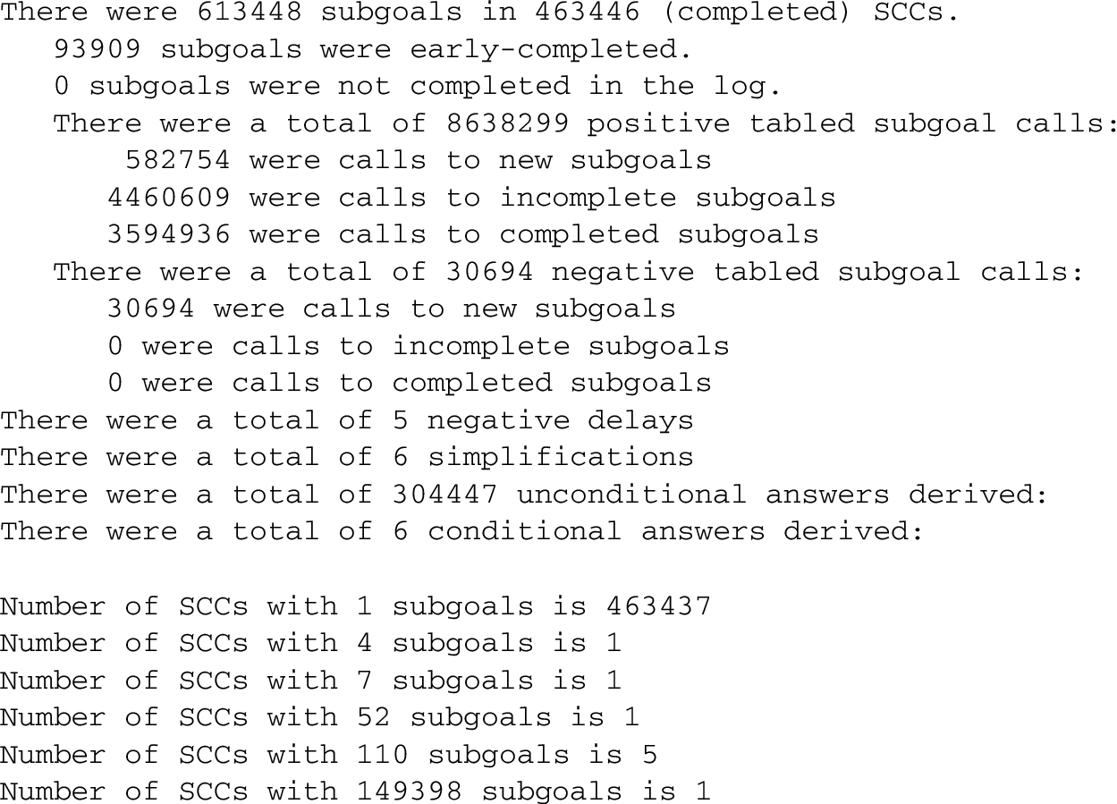
Output of Forest Log Overview for the Program and Query in Example 1.1.

The forest log overview first shows the total number of completed and non-completed subgoals and SCCs, along with a count of how many of the completed subgoals were early-completed (Section 2.1). Information about non-completed subgoals is useful for analyzing computations that do not terminate. The overview also distinguishes between positive and negative calls to tabled subgoals, and for each such class further distinguishes subgoals that were new, completed, or incomplete. Recall that calls to completed tabled subgoals essentially treat the answers in the table as facts, so that such calls are efficient. Making a call to an incomplete subgoals on the other hand means that the calling and called subgoals are mutually recursive;14 ¹⁴

This statement is true not only in local evaluation but also in another common scheduling strategy called batched evaluation.

and execution of recursive sets of subgoals can be expensive, especially in terms of execution stack space. Aggregate counts of delaying and simplification are also given along with counts of both conditional and unconditional answers. Negation does not appear to play a major role in this computation, and it appears likely that the portion of the program relevant to the query has a 2-valued well-founded model, although further exploration would be needed to determine this (cf. Section 4.3).

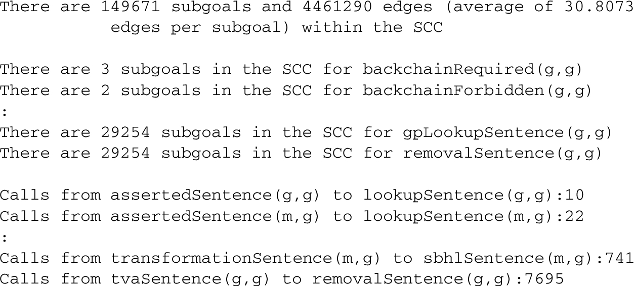
The overview also provides the distributions of tabled subgoals across SCCs formed by the SDGs of the various forests in the evaluation. While most of the SCCs were small, one was very large with nearly 150,000 mutually dependent subgoals. Clearly the large SCC should be examined. The first step is to obtain the index of its SCC (a unique integer that denotes the SCC). The query get_scc_size(Index,Size), Size > 1000. indicated that the index of the large SCC was 39. The query analyze_an_scc(39) then provided the information in Fig. 7.15 ¹⁵

For the purpose of space, the lists of predicates and edges in the SCC have been abbreviated.

For this, SDG information was extracted from the log and this information was analyzed. It is evident from the count of edges in the first line of this report that the vast majority of the calls to incomplete tables during this computation occurred in the SCC under investigation. Since information on incomplete tables is kept in XSB’s choice point stack (cf. [17]), the evaluation of SCC 39 is the likely culprit behind the large amount of stack space required. The subgoals in the SCC are first broken out by their predicate name and arity, then the edges within the SCC are broken out by the predicates of their caller and called subgoals. Figure 7 contains a number of predicates used to encode Cyc’s reasoning into XSB, such as lookupSentence/3, forwardSentence/3 and others. A programmer can review the various rules for these predicates to determine whether the recursion is intended and if so, whether it can be simplified. In the actual example, examination of these rules showed that the use of Hilog resulted in calling a number of unexpected predicates. Additional guards were placed on the Hilog call, greatly reducing the time and space needed for the computation.

Fig. 7.

Output of SCC Analysis for the Program and Query in Example 1.1.

4.2. Using abstraction in the analysis

Within the SCC analysis, information about a given tabled subgoal S is abstracted: only the functor and arity of S is presented. For SCC 39 in the running example, abstraction is necessary, as directly reporting 150,000 subgoals or 4,000,000+ edges would not provide a human with useful information. However, it could be the case that seeing the tabled subgoals themselves would be useful for a smaller SCC. Even for a large SCC, it can be useful for different levels of abstraction to provide mode or type information. For this reason, forest log analysis predicates support calls such as analyze_an_scc(39,abstract_modes(_,_)) which applies the predicate abstract_modes/2 in the breakdowns of subgoals and edges. abstract_modes(In,Out) simply goes through each argument of the term In and unifies the corresponding argument of the term Out with

v if the argument is a variable;

g if the argument is ground; and

m (for mixed) otherwise.

The resulting output is shown in Fig. 8. Examination of this output indicates that the SCC consists of a large number of fully ground calls to several predicates: rewriting code to make fewer but less instantiated calls to these predicates will often optimize a computation in such cases.

Fig. 8.

Output of SCC Analysis for the Program and Query in Example 1.1.

Of course, abstract_modes/2 is simply an example: term abstraction predicates are easy to write, and any such predicate may be passed into the last argument of analyze_an_scc/3.16 ¹⁶

Due to its use of Hilog, Flora-2 terms are all instances of the generic predicates apply/[1,…,n]. Accordingly, abstraction was used to break out predicate-level information in the output of Section 4.1, while a special version of abstract_modes/2 was used here.

4.3. Analyzing negation

Many programs that use negation are stratified in such a way that they do not require the use of delaying and simplification operations. However if a program does not have a two-valued a well-founded model, a user would often like to understand why this is. Even in a program that is two-valued, the heavy use of delaying and simplification can indicate that some rules may need to be optimized by having their literals reordered.

As indicated previously, the forest log overview includes a total count of delaying and simplification operations, as well as a count of conditional answers. In addition, SCC analysis counts negative as well as positive edges within the SCC. Forest logging also provides an analysis routine to examine why answers have an undefined truth value. Recall from Example 2.2 that there are two types of causes of an undefined truth value: either 1) a negative literal explicitly undergoes a delaying operation; or 2) a conditional answer may be used to resolve a literal. It can be shown that in local evaluation, a conditional answer A will never be returned out of an SCC if A is successful or failed in the well-founded model of a program. This means that the operational cause making an answer for S undefined is either a delaying operation within the SCC of S; or a delaying operation within some other SCC on which S depends. So to understand why an atom is undefined it can be useful to understand the “root causes” of the delay: that is, to examine SCCs in which delaying operations were executed and conditional answers were derived, but where the answers could not be simplified.

Example 4.1.

As a use case, logging was made of execution of a Flora-2 program that tested out a new defeasibility theory (cf. [20]). The forest log overview indicated that the top-level query was undefined:  :  There were a total of 55 negative delays  There were a total of 0 simplifications  There were a total of 695 unconditional                           answers derived  There were a total of 66 conditional                           answers derived

The analysis predicate three_valued_scc(List) produces a list of all SCC indices in which delaying caused the derivation of conditional answers. These SCCs were then analyzed as discussed in the previous sections.

5. Implementation and performance of logging and analysis routines

A user of XSB may invoke forest logging so that the log is created as described in Section 2. Alternately, a user may invoke partial logging. This option omits facts produced by the answer resolution operation, which returns an answer to a node with a selected literal that is tabled. Partial logging can save time and space while supporting analysis of mutually recursive components as in Sections 4.1 and 4.2. However it does not support the negation analysis of Section 4.3.

Regardless of the level that is enabled, logging is performed by conditional code in large virtual machine instructions of XSB’s engine, the SLG-WAM, such as tabletry (new subgoal), answer_return, new_answer and check_completion (completion) (cf. [17]). Subgoals and bindings are then written using registers, tables, answer templates, and lists of delayed literals. Access to calling subgoals (e.g., the second arguments of tc/4 and nc/4) is obtained by the SLG-WAM’s root subgoal register, which was originally introduced for tabled negation [17]. For efficiency, logging minimizes interaction with the operating system: information is written into internal buffers; once the buffers contain all information for a log fact, they are written to the output stream using a single printf() statement. The subgoals and answers that are logged may be quite large, particularly when non-termination may be an issue: thus all buffers used are automatically expandable. The current implementation of forest logging also handles cyclic terms, and terms with attributed variables.

All facts are written canonically17

¹⁷

In Prolog, canonical syntax does not allow operator declarations so that with the exception of list symbols, all function symbols are prefixed and their arguments fully parenthesized. In addition all numbers are written in base 10.

so that loading a log exploits XSB’s efficient reading and asserting of canonical dynamic code. The cmp/3 (completion) facts are trie-indexed (cf. [19]), while most other facts index on multiple arguments. For instance, ar/4 (answer resolution) facts are indexed on their second and third arguments (calling and called subgoals), so that indexing is used if either argument is bound. For each argument, a type of indexing in XSB called star-indexing is used, which can index on up to the first four positions of a given argument [19].

Analysis routines are written in standard Prolog with one exception. Counting the number of (abstracted) edges in an SCC makes use of the code fragment

tc(T1,T2,incmp,_Ctr),

check_variant(cmp(T1,S,_),1),

check_variant(cmp(T2,S,_),1)

The predicate check_variant(Goal,DontCareNum) is implemented only for trie-asserted code (e.g., cmp/3). If Goal is an atom for predicate p/n, check_variant/2 determines whether a variant of the first N – DontCareNum arguments of Goal is in the trie for p/n. The check_variant/2 predicate is implemented in C, and directly traverses the C-based data structures used by XSB to represent tries. check_variant/2 begins matching the leftmost element of a term t with the root of the trie, and proceeds to match each subsequent symbol with a child node of the current trie position; if no match is found check_variant/2 fails. As a result, only a single path from the root need be examined in order to determine whether a variant of tis in the trie. On the other hand, for large SCCs in which there are numerous subgoals that may unify with one another (but aren’t variants), a Prolog search for variance may be subject to a great deal of backtracking, and the time required may be proportional to the size of the trie, rather than to the size of t as with check variant/2. Not surprisingly, the use of check variant/2 is critical to a good analysis time. For example, in the analysis of SCC 39 for the Cyc example presented above, the use of check_variant/2 reduced the time for the forest log overview over 100-fold.

5.1. Performance

Table 1 shows performance results for logging and analysis of various sets of examples:

• Cyc Series. Cyc 1 is the working biology example used throughout this paper; Cyc 3 is a similar, but larger, biology example, Both systems are based on the translation of the Cyc inference engine into Flora-2 and then into XSB.

• Pref-kb Series. Pref-kb contains a small set of tabled Prolog rules about personal preferences that demonstrate reasoning about existential information in a manner similar to description logics, and make use of default and explicit negation. Queries to these rules were run over sets of 3.7 million and 14.8 million base facts.18

  ¹⁸

  Details of this series, including the code used to generate the datasets, are available at sites.unife.it/ai/termination.

  Reach N Series. This series tests logging of an open query to the right-recursive reach/2 predicate in Fig. 1 over fully connected graphs with 2000–12000 nodes. Since these queries measure reachability from all nodes in the graphs the cost of an open query scales quadratically with respect to the number of nodes in the graph. Although the tabling behavior of a simple transitive closure query such as reach/2 is well understood, this series is included to test the scalability of logging and of its analysis.

  Table 1

  Timings for Loading and Analyzing Logs

  Program	Number of facts	Load time (secs)	Load Space (bytes)	Forest Log Overview (secs)
  Cyc 1	14,009,602	140.1	7,857,572,736	22.1
  Cyc 3	66,256,186	612.2	36,950,074,144	92.2
  Pref-kb 3.7	2,500,193	16.5	725,972,288	2.3
  Pref-kb 14.8	8,000,140	52.5	2,336,039,512	7.3
  reach 2000	12,006,002	78.4	2,496,927,880	8.4
  reach 4000	48,012,002	280.1	9,985,835,352	13.2
  reach 8000	192,024,003	1227.7	39,940,961,128	59.7
  reach 12000	432,036,000	2332.9	89,864,542,056	132.8

  5.1.1. Load time

  In part because of XSB’s library predicates for loading canonical dynamic facts, XSB’s load time is efficient for the various types of logs, loading approximately 100,000 facts per second for the Cyc series, over 150,000 facts per second for the Pref-kb series, and nearly 200,000 facts per second for the reach N series. After being loaded, the Cyc examples took about 500 bytes per fact, the Pref-kb examples about 300 bytes per fact, and the reach N facts about 200 bytes per fact. Much of this space is due to the heavy indexing of log facts. The reason that the Cyc logs take the longest to load and the most space to represent is due to the fact that the subgoals and answers for this benchmark were generated by Flora-2 compilation. For instance, the Hilog transformation used by Flora-2 transforms n-ary predicates and function symbols to $\mathit{n}+1$ ary predicates and function symbols. As a slightly simplified instance, a term such as p(a,f(b),1) is converted to flora_apply(p,a,flora_apply(f,b),1). In addition, Flora-2 represents module information as an additional argument of each atom, requiring further space.

5.1.2. Analysis time

Once the log has been loaded, the indexing makes analysis fast enough to be interactive: for the Cyc biology example the top level analysis took around 22 seconds, and analyzing SCC 39 took about 20 seconds when the built-in predicate-arity abstraction was used, and about 60 seconds for the parameterizable version that used abstract_modes/2. Although computing the forest log overview requires several table scans in addition to indexed retrievals, timings for both the Pref-kb and the reach N series show a sublinear growth of analysis time with respect to log size.

5.1.3. Logging overhead

The overhead of query evaluation was also measured, i.e., the time it took to execute a query when forest logging was turned on, compared to no logging. At a general level it is easy to see that forest logging imposes an overhead on an evaluation that is a constant factor. Within XSB’s virtual machine, the SLG-WAM, calls to functions that write log facts are placed directly in tabling instructions and never cause any path through an instruction to be re-executed. The cost of logging a given fact is bounded by a factor that is constant for each terminating evaluation $\mathcal{E}$ . Let $\mathcal{E}$ require execution of n instructions in XSB’s virtual machine, and let s be the maximal size of any tabled subgoal in $\mathcal{E}$ . The maximal cost of traversing each logged fact can be treated as a linear function of the maximal subgoal size, s, and the maximal number used for the counter, n. Thus, for a given evaluation $\mathcal{E}$ with s and n fixed, the cost of, e.g., tc/4 is the constant function $2\mathit{s}+\mathit{n}$ .19

¹⁹

Full details would require a lengthy exposition of low-level details of the implementation of forest logging with XSB’s virtual machine.

Of course, even an overhead that is a constant factor can have practical importance. For the Cyc series, the overhead of logging increased the time for Cyc 1 by 72% and for Cyc 3 by 132% which was considered acceptable by knowledge engineers. Similarly, the Pref-kb series, which uses a heavily tabled Prolog program, has an average logging overhead of about 225%. On the other hand, for the reach N series the overhead of forest logging on query execution was naturally high (about 2 orders of magnitude), as reach N performed very little program clause resolution. This overhead may be considered as representative of a worst-case for forest logging overhead.20 ²⁰

The reach N series was included to benchmark scalability, but partial logging as described in the next section can greatly reduce the logging overhead and log space of the reach N series, if needed.

5.1.4. Partial logging

For some large examples, partial logging (mentioned at the beginning of this section) can reduce the logging overhead, the time required to load a log, and the space the loaded log requires. An example of this is as follows.

Example 5.1.

In analyzing the log for a query to Pref-kb, it became apparent that much of the resources the query required were due to large SCCs composed almost entirely of goals to equals/2, the predicate used for equality of non-identical terms. By examining the program, a rule for equals/2 was translated from a right-recursive form to a left-recursive form. Simplifying somewhat, this meant translating a rule of the form:

equals(X,Z):-basePredicate(X,Y),equals(Y,Z)

to

equals(X,Z):-equals(Y,Z),basePredicate(X,Y)

The left-recursive form is usually faster for tabled Prolog, as Prolog’s left-to-right literal selection strategy means that the right-recursive form will generate separate tabled queries for different instantiations of Y while the left-recursive form will not.

After performing the above translation, the query time for the transformed series, Pref-kb-lr was reduced by 300–400%, and the maximum memory required for query evaluation was reduced by about 700–800%. However, while the translation optimized the query itself, when logging was turned on the left-recursive query slowed down substantially, even compared to the time required by the right-recursive form when using logging.

Inspection of the log for the query to left-recursive Pref-kb showed that a large number of answers were produced for the top-level query and its tabled subqueries. Since partial logging removes most information about answer derivations it can substantially reduce the logging time and log size for queries with a large number of answers. Table 2 shows that partial logging reduces the size of the log for left-recursive Pref-kb by many orders of magnitude. On the other hand, evaluation of the query to right-recursive Pref-kb produces a large number of subgoals and relatively few answers, so that partial logging is not more efficient than full logging in this case.21 ²¹

Although the left-recursive and the right-recursive forms of Pref-kb are semantically equivalent, the left-recursive form makes fewer queries than the right-recursive form but its queries are not as instantiated. The left-recursive form thus has a larger search space than the right-recursive form, but it creates far fewer queries for its search and for that reason is more efficient under XSB’s tabling implementation.

Table 2

Comparing Full and Partial Logs for Pref-kb: Times are in Seconds and Space is in Bytes

equals/2 form	EDB Size	Log Level	Log Overhead	Nbr of facts	Load time	Load Space	Forest Log Overview
Right-recursive	3.7 million	full	236%	2,500,254	16.5	725,972,288	2.3
Right-recursive	3.7 million	partial	236%	2,500,126	16.5	724,037,016	2.3
Left-recursive	3.7 million	full	2685%	11,983,203	89.3	3,904,201,328	1.1
Left-recursive	3.7 million	partial	<1%	115	<0.1	80,202	<0.1

6. Related work

Trace-based analysis has been widely used to analyze the behavior of concurrent systems, security vulnerabilities, suitability for optimization strategies and other program properties. Within logic programming, it has been used to support debugging of Prolog [5], Mercury [6], and evaluations that make use constraint-based reasoning [7,14]; the trace analyzer for Mercury was extended to support synchronous program monitoring [11]. More recently, a well-known use of trace-based analysis is the Ciao pre-processor, which infers call and success conditions for a variety of domains based on execution of queries (see [10] for further details).

Based on XSB’s forest logging, a system for analyzing non-termination of Flora-2, Silk and Ergo programs, called Terminyzer has been developed [15]. In addition to the logging mechanisms described so far, Terminyzer relies on special routines that translate compiled Flora-2 code back from a Prolog syntax to a more readable Flora-2 syntax. Displays for Terminyzer are shown in the IDEs of both Silk and Ergo and have been used for debugging by knowledge engineers [1]. The analysis presented in Section 4 predates the termination analysis of [15], and is complementary to it. For instance, the analyses in Section 4.1 considered a program and query that terminated, but was inefficient due to unexpected dependencies among subgoals; while the negation analysis of Section 4.3 helped indicate why a 2-valued model was not obtained.

7. Discussion

The design of a forest log attempts to balance the amount of information logged against the time it takes to load and analyze a log. The propositions of Section 3 show that a forest log suffices to analyze dependency information and, under certain conditions, has the information available to construct a homomorphic image of an SLG forest. The analysis predicates of Section 4 show how the representation is used to provide meaningful information to users about tabled programs with and without negation. The benchmarks of Section 5 further demonstrate practicality of this approach and its scalability to logs consisting of hundreds of millions of facts. As a result forest logging is now fully integrated into XSB and Flora-2, and underlies tools in the commercial Silk and Ergo IDEs.

More generally, trace-based analysis provides an alternative to static analysis for a number of program or query properties. Unlike static analysis, trace-based analysis requires realistic data along with a representative set of queries. On the other hand, for programs that include Hilog, defeasibility, equational reasoning and other features of Flora-2, Ergo and Silk, static analysis techniques may not exist, may not be implemented, or may not be powerful enough for practical use. As a result, trace-based analysis is a viable technique to determine properties of large tabled computations.

An interesting direction for future work involves having a separate process (or thread) monitor the forest log as the information is produced (cf. [11]). Depending on the application, a monitor may need to retain only a small portion of the log and so would reduce the sometimes significant load and analysis times for a full log. An even more intriguing extension would be to have the monitor communicate back to the execution engine to adapt tabling definitions to ensure termination or to improve efficiency.