Data science skills: Building partnership for efficient school curriculum delivery in Africa

Abstract

Data science is a concept to unify statistics, data analysis, machine learning and their related methods in order to analyze actual phenomena with data to provide better understanding. This article focused its investigation on acquisition of data science skills in building partnership for efficient school curriculum delivery in Africa, especially in the area of teaching statistics courses at the beginners’ level in tertiary institutions. Illustrations were made using Big data of selected 18 African countries sourced from United Nations Educational, Scientific and Cultural Organization (UNESCO) with special focus on some macro-economic variables that drives economic policy. Data description techniques were adopted in the analysis of the sourced open data with the aid of R analytics software for data science, as improvement on the traditional methods of data description for learning and thus open a new charter of education curriculum delivery in African schools. Though, the collaboration is not without its own challenges, its prospects in creating self-driven learning culture among students of tertiary institutions has greatly enhanced the quality of teaching, advancing students skills in machine learning, improved understanding of the role of data in global perspective and being able to critique claims based on data.



1. Introduction

Data science is a “concept to unify statistics, data analysis, machine learning and their related methods” in order to “understand and analyze actual phenomena” with data. It employs techniques and theories drawn from many fields within the context of mathematics, statistics, computer science, and information science.

Data Science has spread its branches through several quintessential fields in modern day learning. It has emerged as a global phenomenon that has revolutionized industries and has increased their performances substantially [1]. Given the vast increase in the volume and complexity of data and the new technologies that have been developed to process and analyze this information, it can be argued that there is an increased need for statistical thinking in the context of working with data [2]. Key statistical reasoning topics that are critical for Data Scientists to know at a deep level include but are not limited to the following: developing clear statements of the problem/scientific research question; ensuring acquisition of high-quality data; understanding the process that produced the data, to provide proper context for analysis; allowing domain knowledge of the problem to guide both data collection and analysis; approaching modeling as a process that requires an overall strategy.

The modern day “romance” between Data Science and Statistics cannot be overemphasized (see Fig. 1). Statistics can be a powerful tool when performing the art of Data Science. From a high-level view, statistics is the use of mathematics to perform technical analysis of data. A basic visualization such as a bar chart might give some high-level information, but with statistics one gets to operate on the data in a much more information-driven and targeted way. The analysis involved helps to form concrete conclusions about our data rather than just guesstimating. Using statistics, we can gain deeper and more fine grained insights into how exactly our data is structured and based on that structure, optimally apply other data science techniques to get even more information [3].

Figure 1.

The interactive disciplines of data science.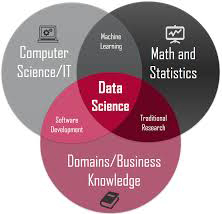

Education is the key to shaping the lives of people. Since the dawn of civilization, humans have evolved through education and have developed mechanisms to improve education. In the 21st century, where data is omnipresent in every walk of life, education is no exception. With advancements in computing techniques, it is possible to imbibe all the information through powerful big-data platforms [4]. Various Schools have to keep themselves updated with the demands of the industry so as to provide appropriate courses to their students. Furthermore, it is a challenge for the Schools to keep up with the growth of industries. In order to accommodate this, Schools are using Data Science systems to analyze growing trends in the market [5]. Using various statistical measures and monitoring techniques, data science can be useful for analyzing the industrial patterns and help the course creators to imbibe useful topics. Furthermore, using predictive analytics, Schools can analyze demands for new skill sets and curate courses that address them [6].

The performance of students depends on the teachers. While there are many assessment techniques that have been used to assess the performance of teachers, it has been mostly manual in nature. With the breakthrough in data science, it is possible to keep track of the teacher performance. This is not only valid for recorded data but also real-time data. As a result, with real-time monitoring of teachers, rigorous data collection is possible, along with its analysis. Furthermore, we can store and manage unstructured data like student reviews on a big data platform.

1.1 Data science and statistics curriculum

A growing number of students are completing bachelor’s degrees in statistics and entering the workforce as data analysts. In these positions, they are expected to understand how to use databases and other data warehouses, scrape data from Internet sources, program solutions to complex problems in multiple languages, and think algorithmically as well as statistically [7]. This increase in the number of undergraduates may help address the impending shortage of quantitatively trained workers. Statistics graduates at the bachelor’s level often work as analysts, and as a result need training in statistical methods, statistical thinking and statistical practice; a foundation in theoretical statistics; increased skills in computing and data-related technologies; and the ability to communicate [6, 7]. Computing skills to enable processing of large data sets are particularly relevant, as noted in the recent London Report on the Future of Statistics. Much of the statistics education literature focuses on the introductory statistics course and statistics before college. Given the relatively few decades since the establishment of undergraduate statistics programs, this is not surprising. While there has been impressive growth in the number of students taking introductory statistics, there has been a relative dearth of articles on the curriculum beyond the introductory course [8].

The digital age is having a profound impact on statistics and the nature of data analysis, and these changes necessitate revaluation of the training and education practices in statistics. Computing is an increasingly important and necessary aspect of a statistician’s work, and needs to be incorporated into statistics [9]. Successful statisticians must be familiar with the computer, for they are expected to be able to access data from various sources, apply the latest statistical methodologies, and communicate their findings to others in novel ways and via new media. In addition, researchers exploring new statistical methodology rely on computer experiments and simulation to explore the characteristics of methods as an aid to formalizing their mathematical framework [10, 11, 12].

Thus, for the field of statistics to have its greatest impact on policy and science, statisticians must seriously reflect on these major changes and their implications for statistics education. Faculty of science in African higher institutions needs to indicate to students that computing and data science is an important element of their statistics education, and it must be taught with an intellectual foundation that provides students with skills to reason about important computational tasks and continue to learn about new computational topics in statistics and Data science. Instead of teaching similar concepts with varying degrees of mathematical rigor, statisticians need to address what is missing from the curricula and take the lead in improving the level of students’ data competence. It is our responsibility, as statistics educators, to ensure our students have the computational understanding, skills, and confidence needed to actively and whole-heartedly participate in the computational arena.

Based on the discussion above, traditional statistics is the basis of data science, but there should be some improvement in the statistics curriculum. These changes are necessary in order to attract and prepare future statisticians, and to keep pace with the rapidly changing “big science” fields. As the practice of science and statistics research continues to change, its perspective and attitudes must also change so as to realize the field’s potential and maximize the important influence that statistical thinking has on scientific endeavors.

2. Materials and methods

2.1 Materials

Social-economic panel data spanning between year 1999 and 2018, consisting of variables GDP at Purchasing Power Parity (PPP) per capita (constant 2011 international $), GNI per capita based on PPP and Official Exchange rates of sixteen Eq. (16) West African countries as published by United Nations Educational, Scientific and Cultural Organization (UNESCO), was used for data description and visualization in R-statistical software for data science. This made the dataset (named as social.csv) to contain 320 rows and 4 columns. The data frame includes the following columns with description:

Variable Country relates to each of the West African countries as two letters abbreviation. A factor with levels: BJ, Benin; BF, Burkina Faso; CV, Cape Verde; GM, Gambia; GH, Ghana; GN, Guinea; GW, Guinea Bissau; CI, Cote d’Ivoire; LR, Liberia; ML, Mali; MR, Mauritania; NE, Niger; NG, Nigeria; SN, Senegal; SL, Sierra Leone; and TG, Togo was used to represent those countries as published by UNESCO.

Variable GDP at PPP per capita is the Gross Domestic Product adjusted for inflation. It relates to the total monetary or market value of all finished goods and services produced within countries borders in a specific period of time divided by the average (or mid-year) population for the same year.

Variable GNIPC based on PPP (US$) is referred to as the Gross National Income Per Capita based on the Purchasing Power Parity rates. It is the gross national income, converted to US dollars using the PPP rates.

Variable ER is shortened as Exchange Rate. It is the value of the selected West Africans currencies in relation to the United States’ (US$) currency.

These variables were used to explain the data description techniques to the students, which also serves as a mean of driven their knowledge on the usefulness of socio-economic indicators.

2.2 Methods

Descriptive Statistics: Descriptive statistics is the first technique used to represent nearly every dataset as they form the foundations for more complicated computations. R sets of commands were generated for the statistics and used to calculate summary statistics, including mean, standard deviation, range, quartile and percentilepercentile as expressed in the following equations:

Arithmetic Mean: The arithmetic mean of observations $x_1,x_2,\mathrm{\dots }{x}_n$ for ungrouped data is given by

$\overline{x}={\displaystyle \frac{1}{n}}{\displaystyle \sum _{i=1}^n}{x}_i\hspace{1em}i=1,2,\mathrm{\dots },n$(1)

For grouped data, we have

$\overline{x}={\displaystyle \frac{1}{{\sum }_{i=}^n{f}_i}}{\displaystyle \sum _{i=1}^n}{f}_i{x}_i\hspace{1em}i=1,2,\mathrm{\dots },n$(2)

Where $f_i$ is the frequency of each observations.

Median: The middle value after a set of observations $x_1,x_2,\mathrm{\dots }{x}_n$ is arranged in order of magnitude is given by

$x_{\text{𝑚𝑒𝑑}}={\displaystyle \frac{1}{2}}(n+1)\mathit{\text{th}}\text{observation}$(3)

Equation (3) is used when the number of observation is odd. But when the number of observation is even, we have

$x_{\text{𝑚𝑒𝑑}}={\displaystyle \frac{1}{2}}[\left({\displaystyle \frac{1}{2}}\mathit{\text{nth observation}}\right)$ (4) $\mathrm{\hspace{1em}}+{\displaystyle \frac{1}{2}}(n+1)\mathit{\text{th}}\text{observation}]$

For grouped observations with corresponding frequencies $f_1,f_2,\mathrm{\dots },f_n$ , we have

$x_{\text{𝑚𝑒𝑑}}=L_1+\left[{\displaystyle \frac{\frac{1}{2}N-\sum f^{*}}{f_m}}\right]C$(5)

Where; $L_1$ is the lower class boundary of the median class; $N$ is the total observations under consideration; $\sum f^{*}$ is the cumulative of the frequencies preceding the median class; $f_m$ is the frequency of the median class. However, the median class is determined by the class to which $\frac{1}{2}n$ falls in the cumulative frequency column.

Variance: The variance of observations $x_1,x_2,\mathrm{\dots }{x}_n$ for ungrouped data is given by

$s^2={\displaystyle \frac{1}{n}}{\displaystyle \sum _{i=1}^n}{(x_i-\overline{x})}^2\hspace{1em}i=1,2,\mathrm{\dots },n$(6)

For ungrouped data, we have

$s^2={\displaystyle \frac{1}{{\sum }_{i=}^n{f}_i}}{\displaystyle \sum _{i=1}^n}{f}_i{(x_i-\overline{x})}^2$ (7) $i=1,2,\mathrm{\dots },n$

Square root of Eqs (6) and (2.2) give the standard deviation.

Range (R): Given observations $x_1,x_2,\mathrm{\dots }{x}_n$ , the difference between the maximum and minimum value is referred to as the range. It is given as

$R=\text{max}\mathit{\text{observation}}-\text{min}\mathit{\text{observation}}$(8)

Quartiles: this divides a given set of observations $x_1,x_2,\mathrm{\dots }{x}_n$ into four Eq. (2.2) equal parts given as

$Q_i=L_{Q_i}+\left[{\displaystyle \frac{\frac{1}{4}N-\sum f_{Q_i}^{*}}{f_{Q_i}}}\right]C,$ (9) $i=1,2,3$

Where $Q_i$ is the $i^{\text{th}}$ quartile; $\sum f_{Q_i}^{*}$ is the cumulative frequencies preceding the $i^{\text{th}}$ quartiles class; $f_{Q_i}$ is the frequency of the $i^{\text{th}}$ quartile class; $C$ is the class interval.

Percentiles: This divide a given set of observations $x_1,x_2,\mathrm{\dots }{x}_n$ into hundred (100) parts, give as

$P_i=L_{P_i}+\left[{\displaystyle \frac{\frac{1}{100}N-\sum f_{P_i}^{*}}{f_{P_i}}}\right]C,$ (10) $i=1,2,\mathrm{\dots },99$

Where $P_i$ is the $i^{\text{th}}$ percentilepercentile; $\sum f_{P_i}^{*}$ is the cumulative frequencies preceding the $i^{\text{th}}$ percentiles class; $f_{P_i}$ is the frequency of the $i^{\text{th}}$ percentile class; $C$ is the class interval.

Moments: Given observations $x_1,x_2,\mathrm{\dots }{x}_n$ , the $r^{\text{th}}$ moment about the origin for grouped and ungrouped data is defined by

${\mu }_r={\displaystyle \frac{1}{n}}{\displaystyle \sum _{i=1}^n}{x}^r;r=1,2,\mathrm{\dots },n$(11) ${\mu }_r={\displaystyle \frac{{\sum }_{i=1}^{n}f{x}^r}{{\sum }_{i=1}^{n}f}};r=1,2,\mathrm{\dots },n$(12)

However, the corresponding $r^{\text{th}}$ moment about the mean for ungrouped data is defined by:

${\mu }_r={\displaystyle \frac{1}{n}}{\displaystyle \sum _{i=1}^n}{(x_i-\overline{x})}^r$(13) ${\mu }_r={\displaystyle \frac{1}{{\sum }_{i=}^n{f}_i}}{\displaystyle \sum _{i=1}^n}{f}_i{(x_i-\overline{x})}^r$ (14) $i=1,2,\mathrm{\dots },n$

Equating $r=1,2,3,4,\mathrm{\dots }$ corresponds to first moment, second moment, third moment, forth moment and so on.

Skewness and Kurtosis: Skewness is the measure of departure of a curve from symmetry. The distribution of a set of data is symmetrical if the three measures of central tendencies coincide while Kurtosis is the measure of Peakedness. Students were exposed to how Skewness and Kurtosis of a curve can be measured using method of moments as given below:

${\alpha }_1={\displaystyle \frac{{\mu }_1}{\sigma }}=0$(15) ${\alpha }_2={\displaystyle \frac{{\mu }_2}{{\sigma }^2}}={\displaystyle \frac{{\sigma }^2}{{\sigma }^2}}=1$(16) ${\alpha }_3={\displaystyle \frac{{\mu }_3}{{\sigma }^3}}={\displaystyle \frac{{\mu }_3}{{\mu }_2^{3/2}}}=1$(17) ${\alpha }_4={\displaystyle \frac{{\mu }_4}{{\sigma }^4}}={\displaystyle \frac{{\mu }_4}{{\mu }_2}}=1$(18)

If ${\alpha }_3=0$ , then the distribution is symmetrical, but if ${\alpha }_3<0$ , we have a negatively skewed curve and ${\alpha }_3>0$ indicates a positively skewed curve. ${\alpha }_4$ measures the $4^{\text{th}}$ moment (Peakedness) of the dataset hereinafter referred to as Kurtosis. The criteria is to know if the curve is either Mesokurtic ( ${\alpha }_4=3$ ), Platykurtic ( ${\alpha }_4<3$ ) and Leptokurtic ( ${\alpha }_4>3$ ).

Shapiro Wilk normality Test is a test of normality in frequents statistics. It tests the null hypothesis that a sample $x_1,x_2\mathrm{\dots }{x}_n$ came from a normally distributed population. The test statistic is written as

$W={\displaystyle \frac{{\left[{\sum }_{i=1}^n{a}_i{x}_{(i)}\right]}^2}{{\sum }_{i=1}^n{(x_i-\overline{x})}^2}}$(19)

where $x_{(i)}$ is the ith order statistic and the constants $a_i$ are given by $\frac{m^T{V}^{-1}}{{(m^T{V}^{-1}{V}^{-1}m)}^{1/2}}$ . $m={(m_1\mathrm{\dots }{m}_n)}^T$ .

And $m_1\mathrm{\dots }{m}_n$ are the expected values of the order statistics of independent and identically distributed random variables sampled from the standard normal distribution, and V is the covariance matrix of those order statistics. The null hypothesis may be rejected if W is too small.

3. Results and discussion

The dataset was extracted in MS-excel and was saved as a “comma delimited (social.csv) file”. Another object was created in R for the social.csv file named w_africans as used in exporting the data into the console using the command line:

w_africans $\mathrm{<}$ -read.csv(“social.csv”,header=T)

However, the w_africans dataset was inspected for correctness before commencing the analysis using the commands stated below and the output is as given in Table 1.

Table 1

Output of the first 15 observations of the w_africans dataset

Country period GDPPC_PPP GNIPC_PPP ER
1	BJ	1999	1621.90	1260	615.47
2	BJ	2000	1666.47	1320	710.21
3	BJ	2001	1703.02	1380	732.40
4	BJ	2002	1728.70	1410	693.71
5	BJ	2003	1734.70	1450	579.90
6	BJ	2004	1757.90	1510	527.34
7	BJ	2005	1735.97	1540	527.26
8	BJ	2006	1752.96	1600	522.43
9	BJ	2007	1805.62	1690	478.63
10	BJ	2008	1841.19	1770	446.00
11	BJ	2009	1831.88	1770	470.29
12	BJ	2010	1818.78	1770	494.79
13	BJ	2011	1820.89	1820	471.25
14	BJ	2012	1855.94	1880	510.56
15	BJ	2013	1934.62	1990	493.90

#Displaying the first 15 observations of the w_africans dataset

print(head(w_africans, n=15))

The nature of the columns (variables) in the w_africans dataset was also explored, using

ls(DATAVAR) or names(DATAVAR), where DATAVAR represent the dataframe name to be explored using the commands given below, with the subsequent results.

#Dataset variable names can be viewed using names (dataset) or ls(dataset)

ls(w_africans)

[1] “Country” “ER” “GDPPC_PPP” “GNIPC_PPP”

#Viewing the number of rows and columns in the w_ africans dataset; use ncol(dataset) and nrow(dataset)

ncol(w_africans); nrow(w_africans)

[1] 5

[1] 320

From the results output, the w_africans dataset contains 4 variables and 320 rows as explained earlier

#A more advanced way to view the structure of the dataset is by using str(DATAVAR)

str(w_africans) #Data structure

data.frame’: 320 obs. of 5 variables:

$ Country: Factor w/16 levels “BF”,“BJ”,“CI”,..:2 2 2 2 2 2 2 2 2 2…

$ period: int 1999 2000 2001 2002 2003 2004 2005 2006 2007 2008…

$ GDPPC_PPP: num 1622 1666 1703 1729 1735…

$ GNIPC_PPP: int 1260 1320 1380 1410 1450 1510 1540 1600 1690 1770…

$ ER: num 615 710 732 694 580…

The w_africans data.frame includes 2 numeric variables, 2 integer variables and 1 categorical variable

The Mean value of each of the variables is computed using the commands:

#Calculate the mean of variable with mean(DATAVAR$ VAR): mean of GDPPC_PPP variable

mean(w_africans$GDPPC_PPP, na.rm=TRUE)

[1] 2258.119

#mean of GNIPC_PPP variable

mean(w_africans$GNIPC na.rm=TRUE)

[1] 2117.962

#mean of ER variable

mean(w_africans$ER, na.rm=TRUE)

[1] 857.6926

Here, the average GDP at purchasing power parity per capita, GNI at purchasing power parity per capita and exchange rate (ER) for the 16 West African countries between years 1999 and 2018 is about $2258.12, $2117.962 and 857.6926 per US$ respectively.

Note: The na.rm =TRUE command the console to remove missing value in case there is one.

For the standard deviation, the following commands subsist; and the results represent the spread of the variables.

sd(w_africans$GDPPC_PPP, na.rm=TRUE)#Standard deviation of GDPPC_PPP

[1] 1331.402

$>$ sd(w_africans$GNIPC_PPP, na.rm=TRUE)#Standard deviation of GNIPC_PPP

[1] 1341.855

sd(w_africans$ER, na.rm=TRUE)#Standard deviation of ER

[1] 1596.375

Continuing in the same terrain for the Range computation, minimum and maximum are computed on a single variable using the min(VAR) and max(VAR) formula. Students were taught how to calculate minimums and maximums using the codes below:

#Minimum and maximum GDP of the selected w_ african countries

min(w_africans$GDP, na.rm=TRUE); max(w_africans $GDP, na.rm=TRUE)

[1] 754.86

[1] 6661.99

From the output, the minimum GDP at purchasing power parity per capita is $754.86 and the maximum is about $6,661.99. This indicated a large gap in GDP per capita taking distribution among the West African countries in response to their purchasing power parity into consideration.

$>$ #Minimum and maximum GNIPC of the selected w_ african countries

$>$ min(w_africans$GNIPC_PPP, na.rm=TRUE); max (w_africans$GNIPC_PPP, na.rm=TRUE)

[1] 600

[1] 7330

It can be inferred that the Gross National Income at PPP per capital of all West Africa is between $600 and $7330 inclusive.

#Minimum and maximum ER of the selected w_african countries

min(w_africans$ER, na.rm=TRUE); max(w_africans$ ER, na.rm=TRUE)

[1] 0.27

[1] 9088.32

It is evidenced within the studied periods that Ghana’s economy has not been adversely affected by external forces as shown from their cedis minimum exchange rate to the US$ while the maximum exchange rate of 9088.32 is attributed to Guinea. We can infer that African countries as a nation is still developing and may take some time to meet up with other continents currency rates.

The command “range(VAR)” is used to summarize the minimums and maximums on individual variables. These computations are demonstrated in the following codes:

#Calculate the range of a variable with range(VAR)

range(w_africans$GDPPC_PPP, na.rm=TRUE)#Range of variable GDP

range(w_africans$GDPPC_PPP, na.rm=TRUE)#Range of variable GNDPPC_PPP

[1] 754.86 6661.99

range(w_africans$GNIPC_PPP, na.rm=TRUE)#Range of variable GNIPC_PPP

[1] 600 7330

range(w_africans$ER, na.rm=TRUE)#Range of variable ER

[1] 0.27 9088.32

Students have been taught that a quartile is a value computed from a collection of numeric measurements, showing observation’s rank when compared to all other present observations. Quartile can also be alternatively expressed as a percentilepercentile, as it is identical but on a scale of 0 to 100. Thus, we used quantile() function to obtain quartile and percentile in R, with commands

quantile(VAR, prob=c(prob value1, prob value2, …, prob valuei))

#Calculate the 25th, 50th, 75th percentilepercentile for GDP per capita at PPP

quantile(w_africans$GDPPC_PPP, na.rm=TRUE, prob =c(0.25, 0.50, 0.75, 0.95))

25% 50% 75% 95%

1369.780 1728.700 2851.580 5361.187

From the output, it easily observed that 25% of average GDP at PPP per capita was $136.780 with median (50 ${}^{\text{th}}$ percentilepercentile) of $1728.700; 75% was about $2851.580 and 95% of the African countries have about $5361.187. This may explain the wide gap in GDP growth of each West African countries since GDP per capita is correlated with GNI per capita.

#Calculate the 25th, 50th, 75th percentilepercentile for GNIPC_PPP

quantile(w_africans$GNIPC, na.rm=TRUE, prob=c (0.25, 0.50, 0.75, 0.95))

25% 50% 75% 95%

1195 1680 2625 5435

#Calculate the 25th, 50th, 75th percentilepercentile for ER

quantile(w_africans$ER, na.rm=TRUE, prob=c(0.25, 0.50, 0.75, 0.95))

25% 50% 75% 95%

83.060 494.040 591.740 4528.037

Table 2

Pooled descriptive statistics

Statistic	GDP per capita, PPP ($)	GNI per capita, PPP ($)	ER
Mean	2258.119	2117.965	857.693
Standard Deviation	1331.402	1341.855	1596.375
25 ${}^{\text{th}}$ Percentile (Q ${}_1$ )	1369.780	1195	83.060
50 ${}^{\text{th}}$ Percentile (Q ${}_2$ )	1728.700	1680	494.040
75 ${}^{\text{th}}$ Percentile (Q ${}_3$ )	2851.580	2625	591.740
95 ${}^{\text{th}}$ Percentile	5361.187	5435	4528.037
Minimum	754.860	600	0.27
Maximum	6661.990	7330	9088.32

Source: Extracted from R-console output.

Table 3

Variables normality test

Moments	GDP per capita, PPP ($)	GNI per capita, PPP ($)	ER
Skewness	1.353	1.518	3.283
Kurtosis	4.227	4.940	13.810
Shapiro Wilk Test Statistics	0.848	0.840	0.502
$P$ -value	0.000	0.000	0.0000

Source: Extracted from R-console output.

Students were also taught how to use summary(x) function, where x can be any number of objects, including datasets, variables, and linear models to generate the descriptive statistics of the variables in the dataset. The code is written below for the w_africans dataset with the subsequent results presented below it.

$>$ #Summarize the w_africans dataset using the command summary(x)

$>$ print(summary(w_africans))

Country	period	GDPPC_PPP	GNIPC_PPP	ER
BF:20	Min.:1999	Min.:754.9	Min.:600	Min.:0.27
BJ:20	1st Qu.:2004	1st Qu.:1369.8	1st Qu.:1195	1st Qu.:83.06
CI:20	Median:2008	Median:1728.7	Median:1680	Median:494.04
CV:20	Mean:2008	Mean:2258.1	Mean:2118	Mean:857.69
GH:20	3rd Qu.:2013	3rd Qu.:2851.6	3rd Qu.:2625	3rd Qu.:591.74
GM:20	Max.:2018	Max.:6662.0	Max.:7330	Max.:9088.32
(Other):200		NA’s:1	NA’s:1

The summary outputs provides the descriptive statistics of all objects in the sample dataset and is explicitly presented in Table 2. Further exploration was carried out on the data by checking their respective distributions through Skewness, kurtosis and further test such as the Shapiro wilk test of normality. These were done using the “moments” library in R. Students were taught how to load packages from R as library(). Details are as given below while the summary presented in Table 3:

library(moments)

skewness(w_africans$GDPPC_PPP, na.rm=T) #Skewness coefficient of GDP per capita at PPP

[1] 1.353004

skewness(w_africans$GNIPC_PPP, na.rm=T) #Skewness coefficient of GNIPC at PPP

[1] 1.517567

skewness(w_africans$ER, na.rm=T) #Skewness coefficient of ER

[1] 3.283139

kurtosis(w_africans$GDPPC_PPP, na.rm=T) #Kurtosis coefficient of GDP per capita at PPP

[1] 4.226773

kurtosis(w_africans$GNIPC_PPP, na.rm=T) #Kurtosis coefficient of GNIPC at PPP

[1] 4.940481

kurtosis(w_africans$ER, na.rm=T) #Kurtosis coefficient of ER

[1] 13.80796

shapiro.test(w_africans$GDP)#GDP test of Normality

Table 4

Cross-section data description on average

S/n	Country	CODE	Mean GDP per capita PPP	Mean GNIPC PPP	Mean ER
1	Benin	BJ	1841.461 [141.8469]	1759.500 [330.621]	554.3915 [82.72886]
2	Burkina Faso	BF	1386.965 [213.250]	1320.000 [333.024]	555.261 82.9732
3	Cape Verde	CV	5355.335 [1009.555]	5039.500 [1414.874]	93.1725 [13.51637]
4	Cote D’Ivoire	CI	2913.830 [338.916]	2647.500 [614.524]	555.261 [82.9732]
5	Gambia	GM	1460.178 [40.394]	1349.500 [184.033]	29.855 [10.73796]
6	Ghana	GH	3031.057 [696.137]	2897.500 [969.063]	1.772 [1.346909]
7	Guinea	GN	1735.404 [226.013]	1593.500 [399.569]	5075.988 [2625.065]
8	Guinea Bissau	GW	1430.202 [72.702]	1360.500 [239.109]	555.261 [82.9732]
9	Liberia	LR	1137.824 [136.222]	970.526 [190.860]	71.5625 [24.41597]
10	Mali	ML	1794.605 [151.470]	1670.500 [321.943]	555.261 [82.9732]
11	Mauritania	MR	3348.436 [370.771]	3193.000 [627.259]	28.2255 [4.042962]
12	Niger	NE	823.119 [61.436]	779.500 [138.049]	555.261 [82.973]
13	Nigeria	NG	4565.789 [907.056]	4237.500 [1296.651]	158.823 [61.094]
14	Senegal	SN	2758.823 [263.357]	2614.500 [524.740]	555.261 [82.973]
15	Sierra Leone	SL	1204.011 [243.925]	1158.500 [342.856]	3822.465 [1756.515]
16	Togo	TG	1286.844 [226.013]	1238.500 [399.569]	555.261 [82.9732]

Values in parentheses [ ] represent standard deviation. Source: Extracted from R-console output.

Shapiro-Wilk normality test

data: w_africans$GDPPC_PPP

W $=$ 0.84758, $p$ -value $<$ 2.2e-16

shapiro.test(w_africans$GNIPC)#GNIPC test of Normality

Shapiro-Wilk normality test

data: w_africans$GNIPC_PPP

W $=$ 0.83966, $p$ -value $<$ 2.2e-16

shapiro.test(w_africans$ER)#ER test of Normality

Shapiro-Wilk normality test

data: w_africans$ER

W $=$ 0.5022, $p$ -value $<$ 2.2e-16

Positive coefficients of 1.353, 1.518, and 3.283 indicated that the econometric variables of GDP, GNIPC and ER is highly skewed to the right and may not be normally distributed. As the Kurtosis measure the fourth moments, selected West Africans exchange rate was found to be normally distributed (kurtosis $\approx$ 3) with other kurtosis of other variables $>$ 3, indicating a leptokurtic shape compared to a normal distribution. However, normality test of the data confirmed the non-normality of the data since its associated p-values are lower than 5% level of significance.

Figure 2.

Normal Q-Q plots of GDP at PPP per capita of some selected West African countries.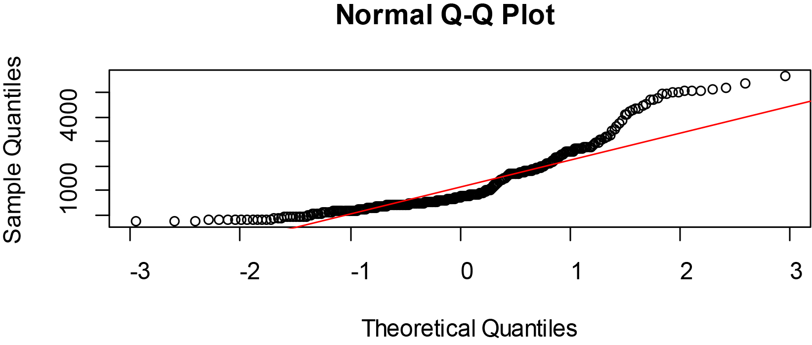

Figure 3.

Normal Q-Q plots of GNI at PPP per capita of some selected West African countries.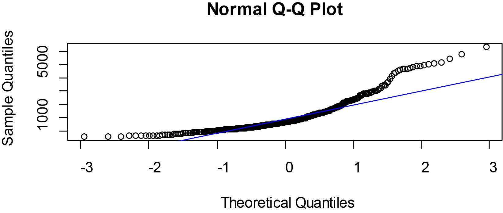

Figure 4.

Normal Q-Q plots of ER of some selected West African countries.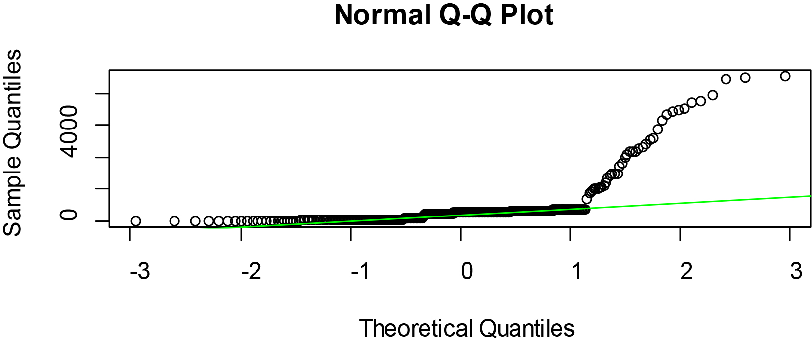

Figure 5.

Bar chart of average GDP per capita based on PPP rates of selected West African countries.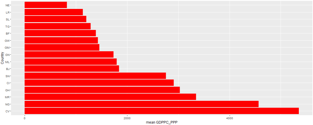

Figure 6.

Bar chart of average GNIPC based on PPP rates of selected West African countries.

Figure 7.

Bar chart of average ER of selected West African countries.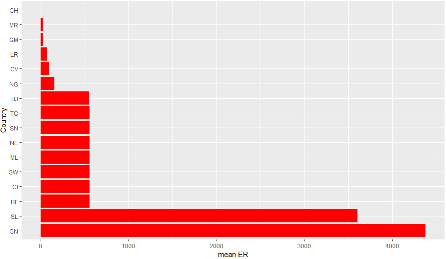

Quantile plots visualize the distribution of the data per variable and details generated by the below commands are as given in Figs 2–4 respectively

par(mfrow=c(2,2)) #Partitioning of plots space

#Quantile plot of GDP per capita at PPP rates

qqnorm(w_africans$GDPPC_PPP);qqline(w_africans$ GDPPC_PPP,col=“red”)

#Quantile plot of GNI per capita at PPP rates

qqnorm(w_africans$GNIPC_PPP);qqline(w_africans$ GNIPC_PPP,col=“black”)

#Quantile plot of Exchange rate

qqnorm(w_africans$ER);qqline(w_africans$ER,col= “green”)#Quantile plot of ER

The Figs 2–4 showed that the quantile plots of the selected variables do not lie on the theoretical normal line. Thus, the variables are not precisely normal but may not be too far off.

Students were also introduced to data splitting in R using dataframe_name[n:m,]. This method was used due to the fact that the data structure was paneled in nature with the first 20 observations on row-wise which represents republic of Benin followed by Burkina Faso, among others. The command line used is given below with the results output presented in Table 4.

benin_d $<$ -w_africans[1:20,];benin_d #Extracted Benin republic variables from the panel structured data.

The data was further explored using ExPanDaR package in R. Average GDP, GNIPC and ER per cross sections (countries) were visualized from the Shiny app using simple bar chart presented in Figs 3–5 respectively.

library(ExPanDaR)

ExPanD(df=w_africans)

The Figs 5–7 showed that Cape Verde (CV) recorded the highest average GDP (per capita) and GNI (per capita) taking into consideration purchasing power parity among the West African countries followed by Nigeria (NG). Cape Verde (CV) also has the highest average GNIPC at purchasing power parity rates and Ghana (GH) possess the strongest currency rate among other west African nations taking the US$ exchange rate into consideration. Niger (NE) recorded the lowest average GDP per capita and GNIPC at PPP and Guinea (GN) with the weakest currency rate within the selected timeframe. This can also be evidenced from Table 4 with an associated variability from the mean.

3.1 Summary of findings

This paper presented students learning experience on the introduction of data science skills for curriculum delivery in Africa using social-economic data extracted from UNESCO website. The interactive session helped students on how to use R software for analyzing for descriptive statistics, and appropriate interpretation of results based on the type of data used for analysis. This bridged the gap between the traditional method of data analysis and the conventional form especially in the area of big data. Findings from the analysis showed that economic growth varies from countries to countries as shown from the pictorial representation of data and respective spread of observation from the mean. However, this result is an indication that Cape Verde (CV) among other West African countries is better off in terms of their economic growth taking purchasing power parity into consideration. This indicated that Nigeria economic growth may be marred by inflation, resulting to the devaluation of her naira note in the international market, among other developing countries. Hence, West African countries in general are far from being developed compared to countries in Asia, America, and Europe to mention a few.

4. Conclusion

Introducing beginner students in statistics to data science is a vexatious task, especially in African countries where regular supply of power is a luxury and uninterrupted internet facilities are quite expensive and almost impossible. The developing nature of most Africa countries has created a paradoxical approach to achieving reasonable success in students’ learning of data science. However, for the purpose of this research, great achievement was made in introducing the students to data description using R software for data science, thereby equipping them with a career in data analysis. From the beginning, students offering introductory statistics gain reasonable experience of what constitutes both the practical and conceptual aspects of the working life of a data scientist, as they were able to run simple codes on exploratory data analysis using the focused data. The students equally enhanced their knowledge in deducing reasonable inference from the output of data analysis. 200 level students were able to run with ease, R codes to estimate basic descriptive statistics within a 1 hour lecture period. The activities was carried out without much supervision on the part of the tutor. Comparison was made per member countries on their developmental rate taking their respective Gross Domestic Product, Gross National Income per capita, and Exchange Rate into consideration.

It is of the opinion that topics covered in data science courses can and should be brought into a variety of statistics courses at undergraduate level, while adequate facilities provided for its teaching and learning. Thus, key data science skills need to be introduced, reiterated, and reinforced throughout the undergraduate statistics curriculum.

Though, the exercise is not without its own challenges, but its prospects in creating self-driven learning culture among students of tertiary institutions has greatly enhance the quality of teaching, advancing students skills in machine learning, improved understanding of the role of data in global perspective and on the spot ability of the students to be able to critique claims based on data.