
Abstract
We developed an error-propagation-analysis-based multi-scale reliability model in three steps to estimate the minimum time-to-failure of a full-size brittle component with environment-assisted crack growth. First, we use a time-to-failure formula according to Fuller et al. (1994), which was based on laboratory experiments on brittle materials for measuring time-to-failure of specimens that undergo moisture-enhanced crack growth under constant stressing. The formula predicted the mean time-to-failure of a specimen-size component in a power-law relationship with the applied stress involving two strength test parameters, S and S v , and two constant stressing test parameters from regression analysis, 𝜆 and N ′ . Second, we use the classical laws of error propagation to derive a formula for the standard deviation of the time-to-failure of a specimen-size component and apply it to computing the standard deviation of the time-to-failure of a specimen-size component for a specific applied stress. Third, we apply the statistical theory of tolerance intervals and develop a conservative method of estimating the failure probability of the full-size components by introducing the concept of a failure probability upper bound (FPUB). This allows us to derive a relationship for the minimum time-to-failure, min-t f , of a full-size brittle component at a specific applied stress as a function f of the FPUB. By equating (1 – FPUB) as the Reliability Lower Bound, RELLB, we arrive at a relation, min-t f = f (RELLB), which expresses the min. time-to-failure as a function of the reliability lower bound, or conservatively as a function of reliability.
Keywords
Introduction
Were it not for the existence of the phenomenon of the environmentally enhanced crack growth, predicting the minimum time-to-failure of brittle components under known stresses would be relatively straightforward, requiring only a statistical estimate of the strength and time-to-failure of the material. Because most brittle materials are subject to slow crack growth in moisture-containing environments under stresses smaller than those leading sudden failure, we must account for this phenomenon in any reliability model development.
In this paper, we develop in three steps an error-propagation-based multi-scale reliability model for predicting the minimum time-to-failure of brittle components with the environment- assisted crack growth phenomenon.
In Section 2, we describe in detail how Fuller et al. [12] developed a lab-scale fatigue-fracture-failure (FFF) model to predict the mean time-to-failure of a specimen-size component in a power-law formula with the applied stress involving two strength test parameters, S and S v , and two constant stressing test parameters from regression analysis, 𝜆 and N ′ . In Section 3, we develop an error-propagation-based lab-scale model by applying the classical laws of error propagation [18] to derive a formula for the standard deviation of the time-to-failure of a specimen-size component. To illustrate how the formula works as a lab-scale model, we introduce in Section 4 three sets of experimental data to estimate the mean and standard deviation of those four parameters, and then apply them to computing the mean and standard deviation of the time-to-failure of a specimen-size component for a specific applied stress.
Based on the lab-scale model that includes effects of measurement uncertainties in material property testing, we develop in Section 5 a new component-scale Reliability model by first applying the statistical theory of tolerance intervals [18,22] and then associating the concept of “Lack of Coverage” with a state of inadequate information in a proportion of the global population of components such that, in the worst case, we can treat that proportion to be in its failure state and the Lack of Coverage becomes the Failure Probability Upper Bound (FPUB). This worst-case scenario allows us to create FPUB estimates and apply a nonlinear least squares logistic function fitting algorithm to derive a formula for the minimum Time-to-failure of a full-size brittle component as a function of FPUB.
In Section 6, we illustrate this new component-scale reliability model with a numerical example where the min. time-to-failure of a full-size component made of BK-7 glass at 20 °C is expressed as a function of reliability. A discussion of the significance and limitations of the new component-scale reliability model and some concluding remarks appear in Sections 7 and 8, respectively.
A lab-scale time-to-failure model of a brittle material with slow crack growth
We begin in this section the first of a three-step modeling methodology to assure safe operation of brittle components undergoing environmentally enhanced crack growth, including a discussion of the methods by which the results of laboratory-scale specimens can be used to predict the reliability of a system of parts. As a demonstration of the feasibility of the first model, we use experimental data obtained on glass intended for aircraft windows [9,12].
Our ability to predict the reliability or lifetime of a brittle part whose strength is likely to degrade with time rests on the use of a mathematical expression (see Freiman et al. [11]) which can represent the crack growth data. Following chemical rate theory which has been shown to be applicable to the environmentally enhanced crack growth process [11], the following exponential relationship between crack velocity, V , and the stress intensity factor, K
I
, has been shown to fit a variety of crack growth data [11]:
Equation (1) can be integrated to yield a time for a flaw to grow from its initial size to the point of failure. However, there are two problems. First, a closed-form solution for integration is difficult to achieve. While such an integration has been reported [19], the integration limits are in terms of flaw size, which from a practical point of view cannot be determined with any degree of accuracy. Second, the effect of a residual stress term associated with the introduction of the flaw has not been incorporated into such an expression [13]. An empirical power law is used instead. A comparison of the fits to data of the two forms has been reported [16].
However, most flaws will experience not only a far-field stress but may also be surrounded by a stress field generated by the impact-type process by which they were introduced, e.g., machining and finishing. Equation (3) is then modified to the following:
Let X = Stressing rate (MPa/s), and Y = Strength (MPa).
Assuming a power law relationship between Y and X, we obtain the following formula:
Let xx = Log X and yy = Log Y. Equation (7) is transformed into the following:
We define 𝜆 and N
′
in terms of the two material parameters, A and C as follows:
The symbol S v is known as the Reference Strength and is estimated in another strength test at a high loading rate in an inert environment.
We now combine Eqs (5) and (6) to obtain a formula for the first time-to-failure model:
S is the initial strength
S v is the strength of an indented reference set of specimens
𝜎 is the tensile stress in the component
𝜆 and N ′ are constants from environmentally enhanced crack growth experiments.
A note on the units of the six quantities described in Eq. (11) is given below:
Unit of t f is s, unit of S, S v , 𝜎 is MPa, unit of 𝜆 is (MPa) N ′ *s, and N ′ is dimensionless.
In the last section, we described a lab-scale model to predict the mean time-to-failure of a specimen-size component in a power-law relationship with the applied stress involving two strength test parameters, S and S v , and two constant stressing test parameters from regression analysis, 𝜆 and N ′ . Estimates of the means and standard deviations of these four parameters from three sets of laboratory tests allow us to estimate their uncertainties. We will now describe the second of our three-step modeling methodology by which the results of laboratory-scale specimens can be used to predict the reliability of a system of parts.
In this section, we develop an error-propagation-based lab-scale time-to-failure model by applying the classical laws of error propagation (see, e.g., Ku [17]) to derive a formula for the standard deviation of the time-to-failure of a specimen-size component.
To compute s.d. (t
f
), we need to apply the variance formulas given by Ku [17] and also in Appendix A (abbreviated due to space limitation) by treating Eq. (11), an algebraic function of expressions involving sum, quotient, product, power, etc., as a telescopic sequence of functions of just two expressions to facilitate the application of the variance formulas. A repeated application of Ku’s formulas yields the following result for the standard deviation of t
f
:
The combination of Eq. (11) of the last section and Eq. (12) above defines the second time-to-failure model, which has incorporated the uncertainty features of the laboratory experimental data but is still a lab-scale model.
Using formulas of variances of elementary algebraic expressions such as sum, product, reciprocal, etc. as listed in Appendix A, we derive formulas for the variances of 𝜆 and N’ from their definitions in Eqs (9) and (10) as follows:
To illustrate how Eqs (11) and (12) work as a lab-scale time-to-failure model, we introduce in this section three sets of experimental data to estimate the means and standard deviations of the four parameters, S, S v , 𝜆 and N ′ , and then apply them to computing the mean and standard deviation of the time-to-failure of a BK-7 glass specimen for a specific applied stress equal to 8.6 MPa.
The initial minimum strength, S, is dependent on the flaw distribution in the material just before it is put into service. In carrying out a reliability analysis, a key assumption is that no flaws more severe than those in the initial flaw distribution are introduced during the lifetime of the part. In addition, it is assumed that flaws grow only due to environmentally enhanced crack growth.
It would be advantageous if the strength distribution of actual parts could be obtained under loading conditions that simulate those during service. However, this can be difficult and costly. Consequently, tests are usually conducted on small pieces of the same material. A key requirement is that the processing procedures and surface treatments, e.g., machining and polishing, of these specimens are identical to that undergone by the part.
Because of the propensity of brittle materials to fail from surface flaws, flexural tests are the primary test method. Such tests can be conducted in either uniaxial or biaxial loading. Because failure from sharp edges is typically a problem with brittle materials the decision of whether to conduct uniaxial or biaxial tests is usually based on whether edges in the part will be subject to significant stresses. If uniaxial testing, e.g., four-point flexure, is chosen, edges should be rounded or chamfered to minimize failure from them. Testing must be conducted at a high loading rate in an inert environment, e.g., dry gaseous nitrogen, to eliminate slow crack growth effects (see, e.g., Ref. [24]). Typically, thirty specimens are recommended to assure that an adequate statistical distribution can be established. However, this value is somewhat arbitrary. The number of specimens needed depends on the scatter in the data and the standard deviation desired. If a component experiences a stress state that could cause it to fail from internal flaws such as pores or inclusions, flexural tests will not be effective, and direct tensile tests will be required.
It is not sufficient to simply calculate a lower limit to failure strength; one must also know the uncertainty in this calculation, particularly its lower bound. The first, and most important, step is to determine the uncertainty in the minimum strength, S, of the set of specimens. In order to determine this uncertainty, one fits the measured strength distribution to a particular mathematical expression. The Weibull function has been used extensively because it is thought to represent the underlying physics governing brittle fracture, namely weakest link theory (see Ref. [2]). The two-parameter Weibull distribution defined in [2] and Eq. (15) below, which allows for failure at zero applied stress, is commonly used partly because of the complexities involved in estimating the uncertainties of the parameters needed for a three-parameter Weibull distribution.
P
f
is the probability of failure; 𝜎 is the stress at fracture; S
0 is known as the Weibull characteristic strength, and m is the Weibull modulus. This is the expression used in most analyses of brittle failure and is the recommended analysis method in an ASTM standard [3]. However, a two-parameter Weibull distribution is both unduly conservative and may not be the best fit to the experimental data (see Fong et al. [7]). The 3-parameter Weibull Eq. (16) below sets a lower limit to the failure strength, S.
The three parameters, S, S 0, and m, in Eq. (16) are known as the Location, Scale, and Shape parameters of the Weibull distribution, respectively.
In Appendix B, we show a list of 31 strength test data for a BK-7 glass material that were published in Fuller et al. [12] for design of aircraft windows. To estimate the three parameters and their standard deviations, we use the Maximum Likelihood (ML) method (see, e.g., Bury [4, pp. 161–168]) in writing a computational code
1
using an open-source statistical software package named DATAPLOT [6]. The results are given in Appendix B, where the Location parameter, S, and its standard deviation, sd(S), are given below:
It follows that the variance of S, Var(S), which equals the square of sd(S), is given by the expression below:
While values of the crack growth parameters, N
′
and 𝜆, can be obtained from direct measurements of crack growth rates, the so-called dynamic fatigue tests [13] employing cracks that are of comparable size to actual flaws in the component are both more convenient as well as relevant to the practical failure issue. As noted earlier, indentations surrounded by a stress distribution led to a more conservative value of the environmental exponent, N
′
rather than N.
S
f
is the fracture strength of a specimen loaded at a constant rate to failure. In the dynamic fatigue test indented flexural bars immersed in water at 20 °C are loaded to failure at a constant stressing rate (Eq. (20)). A linear regression (see, e.g., Draper and Smith [5]) of the log of the fracture strength, S
f
, vs. the log of the stressing rate,
For a BK-7 borosilicate crown glass material, we present in Appendix C a list of strength vs. stress rate (dynamic fatigue) test data of 35 specimens, as reported by Quinn et al. [9], where the list consists of four sub-lists, each of which is distinguished by a nominal stressing rate. For example, by taking the mean of either the stressing rate or the strength as the representative of the nominal stress rate or the nominal strength, we obtain a new list of the dynamic fatigue test data in terms of a nominal strength vs. nominal stressing rate as shown in the table below:
Weighted nominal strength vs. nominal stressing rate
Note that the breaking-up of the list of 35 data points into four sub-lists allows us to estimate the total uncertainty of the dynamic fatigue test data and its two components, namely (a) the short-range stressing rate or intra-rate uncertainty, and (b) the long-range stressing rate or the inter-rate uncertainty. This is important, because our time-to-failure model of Eq. (11) is a static one that works for a fixed applied stress and is independent of the stressing rate. Hence, we are allowed to work only with the long-range rate uncertainty and ignore the short-range one.
In Appendix C, we show not only the list of 35 data points of the dynamic fatigue test of Quinn et al. [9], but also the results of Case 1 (Full Uncertainty) analysis of the data using a linear regression algorithm [5]. In Appendix D, we present the results of Case 2 (Partial-Long Range Rate Uncertainty) analysis of the data given in Table 1 using a weighted linear regression algorithm. For our model of Eqs (11) and (12), it is the analysis of Case 2 that is appropriate for uncertainty estimation. Thus, we obtain from Appendix D the results of the two constants, A and C, and their variances as follows:
Because indented specimens were used to determine N ′ , measurements are needed to normalize the data. These strength measurements, termed S v , must be made at a high loading rate in an inert environment.
In Appendix E, we show a list of 33 reference strength (S v ) test data for a BK-7 glass material that were also published in Fuller et al. [12]. To estimate the three parameters and their standard deviations, we again use the same 3-parameter Weibull DATAPLOT code [6] that was used earlier in estimating the location, scale, and shape parameters of Dataset No. 1.
The results are given in Appendix E, where the Location parameter, S
v
, and its standard deviation, sd (S
v
), are given below:
It follows that the variance of S
v
, Var(S
v
), which equals the square of sd (S
v
), is:
We are now ready to estimate the mean Time-to failure, t
f
, and its standard deviation, sd (t
f
), for an applied max. stress of 8.6 MPa, using Eqs (17), (25), (26), and (29) for evaluating t
f
of Eq. (11) and using in addition all the variances Eqs (19), (27), (28), and (31) for evaluating sd (t
f
) of Eq. (12). The numerical results are as follows:
Lab-scale min. time-to-failure of BK-7 glass component
aThe formula for the half-width of the prediction interval is used for a single future observation.
Note that The availability of an estimate of a standard deviation of the Time-to-failure, sd (t f ), allows us to apply the theory of statistical prediction intervals (see, e.g., Nelson et al. [22, p. 179]) such that, assuming a sample size of n = 31, we obtain the following one-sided lower predictive limits as the predicted Minimum Time-to-failure of any Lab-scale sized component at various levels of confidence:
Note that we purposely highlighted in Table 2 the result of the Lab-Scale Min. Time-to-failure, 5.68 Million-hours, at the 95% level, because as we introduce in the next section the statistical theory of tolerance intervals, we intend to illustrate it with a numerical example to be formulated also at the 95% level of confidence for subsequent comparison of the consequence of applying either the theory of prediction intervals (for Lab-scale modeling) or the theory of tolerance intervals (for Component-scale modeling).
Based on the lab-scale Minimum Time-to-Failure Brittle Fracture Model described in Sections 3 and 4, we develop in this section a new component-scale Fracture-Reliability model by first applying the statistical theory of tolerance intervals (see, e.g., Prochan [23], Natrella [21], Bury [4], and MIL-HDBK-17-1F [25]) and then modeling the concept of “lack of coverage” as a state of inadequate information in a proportion of the global population of components such that, in the worst case, we equate that proportion to its failure probability upper bound (FPUB). This worst-case scenario allows us to construct several FPUB points and apply a nonlinear least squares logistic function fitting algorithm to derive a formula for the minimum time-to-failure of a full-size brittle component at a specific applied stress as a function of FPUB.
To show how the modeling process of converting the “lack of coverage” into the “Failure Probability Upper Bound (FPUB)" works, we illustrate it with a numerical example based on the predicted result of the last section, namely,
To illustrate the above statement, let us assume that we have a sample of size n = 35, and we work with a level of confidence 𝛾 = 0.95. We reproduce in Table 3 a portion of a table in Natrella [21, p. T-15, Table A-7], where one finds the K-factors for different P as follows:
K-factors for one-sided tolerance limits for normal distribution [21]
K-factors for one-sided tolerance limits for normal distribution [21]
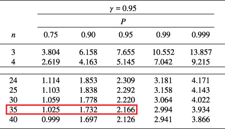
Note that the one-sided Lower Tolerance Limit, LTL, is given by the following equation:
Comp.-scale min. time-to-failure vs. coverage for 𝛾 = 0.95, stress = 8.6 MPa
Note that the theory of tolerance intervals predicts that, for 90% of the global population of glass components at 95% level of confidence, the minimum Time-to-failure, (min-t
f
)com-scale, is 5.52 Million-hours, and that, for 10% of the global population of components and at 95% level of confidence, no estimate of (min-t
f
)com-scale is known. It follows that, in the worst case, the estimate of (min-t
f
)com-scale is zero with the consequence of a failure being predicted for 10% of the global population. Thus, the global population of components is characterized, in the worst case, by a scenario that 10% of it has failed, or its failure probability upper bound (FPUB) is 10% This ends our numerical example for illustrating the modeling process of converting the “Lack of Coverage (1 − P)” into FPUB. In general, our new model for estimating the component-scale minimum Time-to-failure, (min-t
f
)com-scale, is governed by the following two conditions:
In the last section, we developed a new component-scale reliability model by first applying the statistical theory of tolerance intervals [18,22] and then associating the concept of “Lack of Coverage” with a state of inadequate information in a proportion of the global population of components such that, in the worst case, we can treat that proportion to be in its failure state and the Lack of Coverage becomes the Failure Probability Upper Bound (FPUB) as shown in Eq. (35). This worst-case scenario allows us to create several FPUB estimates and apply a nonlinear least squares logistic function fitting algorithm to derive a formula for the minimum Time-to-failure of a full-size brittle component as a function of FPUB.
In this section, we illustrate this new component-scale reliability model with a numerical example to express the minimum Time-to-failure of a full-size component made of BK-7 glass for a specific applied max. stress of 8.6 MPa at 20 °C as a function of reliability.
In order to apply Eq. (35) to create several estimates of FPUB as a function of (min-t f )com-scale, we developed a computer code to generalize Table A-7 of Natrella [21 ] for finding the K-factors of the one-sided Tolerance Limits of a normal distribution as a function of level of confidence, sample size, and coverage (see Heckert and Filliben [14 ,15 ]). Using that computer code, written in DATAPLOT [6 ], we were able to expand our Table 4 to include more values of coverage as follows:
Component-scale min. time-to-failure vs. coverage for 𝛾 = 0.95 and n = 35
Component-scale min. time-to-failure vs. coverage for 𝛾 = 0.95 and n = 35
For modeling (min-t f )com-scale as a function of FPUB, it is more convenient to work with Log(FPUB) as an independent variable. Table 5 becomes Table 6 as shown below:
Component-scale time-to-failure at 8.6 MPa stress vs. Log(FPUB)
In searching for a representation of a min. Time-to-failure, y, vs. Log(FPUB), x, we came upon a 3-parameter logistic function (see, e.g., Forbes et al. [8]), which was originally due to Pierre Francois Verhulst [26] for his use in a study of population growth in 1845. Population growth bears a striking similarity to fracture damage development, which, in turn, resembles the growth of the lifetime of a species from a zero asymptote on the left to a finite positive asymptote to the right. That function looks like an S-curve between two horizontal lines serving as asymptotes with the following equation:
It is worth noting that the concept of reliability or failure probability originated from the days of testing light bulbs, where it was possible to draw a sample of light bulbs from a lot, complete a test for obtaining a failure rate of the sample in a reasonable time frame, and then apply statistical analysis to estimate a failure probability for the lot. For mechanical equipment such as pumps and valves, it is also possible to estimate failure probability from historical failure data if they exist. For most cases in mechanical and structural systems, it is unfortunate that there is not enough historical failure data to allow one to estimate their failure probabilities. The only alternative available today is to conduct failure experiments in a laboratory and develop a model to predict the time to failure in a probabilistic sense, or, as done in this paper, to obtain an upper bound of the failure probability of a component for use in achieving a conservative assessment of the integrity of the component.
Using a nonlinear least squares (NLLSQ), 3-parameter logistic function fit algorithm [5] and a physically-plausible assumption, defined by Eq. (36), that the one-sided Lower Tolerance Limit (LTL), at any confidence level, of the Time-to-failure of a full-size component, cannot be negative, and must approach zero as the lack of coverage, defined as 1 − p, approaches zero, we finally obtain a formula to estimate the minimum Time-to-failure of a component at the full-size scale, (min-t f )com-scale, for any low and extremely low failure probabilities, namely, between 10−2 and 10−7.
Thus, the first and third columns of Table 5 provide the coordinates of four points in a semi-log x-y plot, where the y-coordinate is the (min-t
f
)com-scale, and the x-coordinate is the value of Log(FPUB). In other words, we have the following renaming of variables to implement the model:
For this example, the three parameters are as follows:
A plot of the nonlinear least squares fit based on four points given in columns 1 and 3 of Table 5, is given in Fig. 1. A numerical inversion of the equation given by Eqs (37), (38), (39), and (40) allows us to obtain a plot of Log(FPUB) vs. (min-t f )com-scale at 95% level of confidence, as shown in Fig. 2.
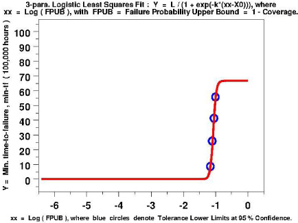
A plot of a nonlinear least squares logistic function fit of four points given in Table 5 where the Y-variable is the min. time-to-failure and the xx-variable is the Log(FPUB).
A change of the scale of the y-coordinate axis from the logarithmic to the natural gives us a plot of FPUB vs. (min-t f )com-scale, as shown in Fig. 3. Since failure probability, FP = (1 – Reliability), we obtain FPUB equals (1 – Reliability Lower Bound), or FPUB = 1 – RELLB, with RELLB = Reliability Lower Bound. This allows us to create a plot of RELLB vs. (min-t f )com-scale, as shown in Fig. 4 and Fig. 5.
For engineering decision making purposes, one can simply replace RELLB by Reliability, and Fig. 4 provides the graphical solution of the reliability modeling problem. The reliability vs. min. time-to-failure curve in Fig. 5 yields Table 7, a table of min. time-to-failure values as a function of reliability at 95% level of confidence:
Component-scale min. time-to-failure of BK-7 glass at 8.6 MPa vs. reliability
Based on Table 7, we observe that the predicted component-scale min. time-to-failure at 95% level of confidence and 90% reliability is 5,474,000 hours for a max. stress of 8.6 MPa. This compares favorably with what was predicted in Section 4 for the lab-scale min. time-to-failure, which at 95% level of confidence is 5,680,000 hours.
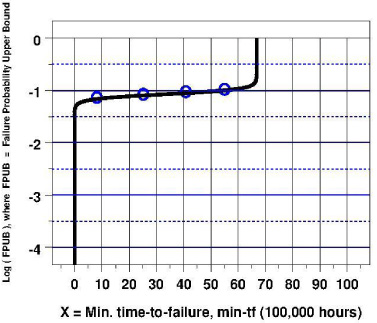
A numerical inversion of the 3-parameter logistic function developed in Fig. 1 allows us to obtain the above plot of Log(FPUB) vs. (min-t f ) com-scale at 95% level of confidence.
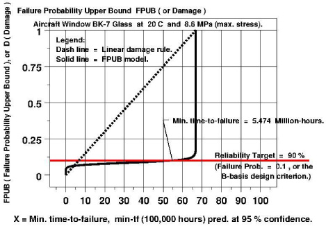
A plot (solid line) of the Failure Probability Upper Bound, FPUB, vs. the Component-scale Minimum Time-to-Failure, (min-t f ) com-scale, at 95% level of confidence, is compared with a plot (dash line) of the linear damage rule when we interpret FPUB as a measure of damage.
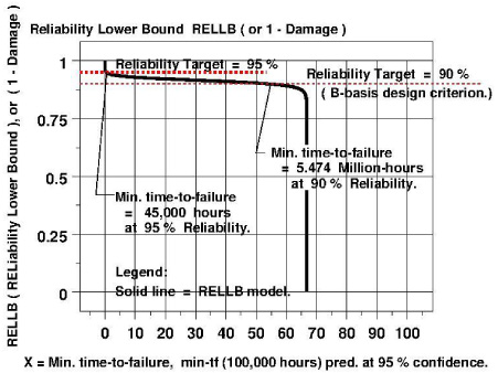
A plot of the Reliability Lower Bound, RELLB, vs. the Component-scale Minimum Time-to-Failure, (min-t f ) com-scale, at 95% level of confidence, based on the solid line plot in Fig. 3 with the relation that RELLB = 1 – FPUB due to the fact that Reliability = 1 – FP.
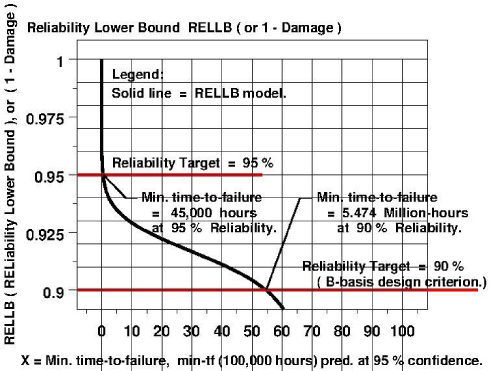
A plot of the Reliability Lower Bound, RELLB, vs. the Component-scale Minimum Time-to-Failure, (min-t f ) com-scale, at 95% level of confidence, based on the solid line plot in Fig. 3 with the relation that RELLB = 1 – FPUB due to the fact that Reliability = 1 – FP.
The prediction of a minimum component-scale time-to-failure of a brittle material such as glass for a specific maximum stress as a function of reliability is significant because it allows engineers to design and operate a brittle component or structure to meet a reliability target as required in some modern engineering codes such as the ASME Boiler and Pressure Vessel Committee Section XI Division 2 Reliability and Integrity Management Code [1].
The modeling methodology for predicting a component-scale minimum time-to-failure of a brittle component is also significant, because the reliability model accounts for uncertainties of all material property parameters and adopts a conservative approach in estimating the failure probability of the components, thus making the prediction more credible and useful. For example, in an earlier paper by Fuller et al. [12], their reliability model used a Monte Carlo method to estimate the min. time-to-failure by accounting for only a limited number of material parameters, and came up with one of their predictions quite different from ours as shown below:
For BK-7 glass at max. stress of 8.6 MPa and 95% level of confidence,
Clearly our model with all uncertainties accounted for provides a more conservative estimate of the min. time-to-failure at the full-size component-scale level. To understand why the two models provide such a drastically different set of results, we need to examine the methods used in each model to account for the uncertainties due to the four material parameters.
In the Fuller’s model [12], a Monte Carlo method using 7,000 sets of combined experimental data involving four material parameters was used with a bootstrap technique to account for the uncertainties of those four parameters. Unfortunately, 7,000 is too few to accurately do the job for 4 random variables, because it would have been fine for one or two random variables, but not for four. A 7,000-Monte-Carlo-set in 4 variables is identical to a random sampling table of a hypercube of dimension 4 with 9 random samplings per variable (9 being approximately the 4th root of 7,000). That means each material parameter was sampled nine times randomly to provide the final result. That number was obviously too small for a Monte Carlo type of exercise to succeed. For a Monte-Carlo method to work, we usually need to sample a single variable at least, say, 100 times. That means 100,000,000 Monte Carlo sets for four parameters, which will make a computer run cost prohibitive. In general, for the number of random variables to be greater than two, Monte Carlo method is not a good choice for dealing with this kind of modeling problem.
On the other hand, our model used the error-propagation-theory method with Eq. (12) showing explicitly how the uncertainty of each material parameter was accounted for. In this sense, we believe our estimate is more credible.
It is important to point out that this reliability model methodology for brittle materials with environment-assisted crack growth is applicable not only to glassy materials as shown in this paper, but also to others such as graphite, provided (a) a laboratory-scale time-to-failure model similar to Eq. (11) and a similar set of experiments that generate three sets of data as shown in Section 4, or, (b) environment-assisted crack growth experiments such as those reported by Freiman and Mecholsky [10] are performed to yield a time-to failure model.
However, our reliability model does have a limitation that needs to be stated, namely, we assumed a power-law relationship for the crack velocity vs. stress intensity factor, as shown in Eq. (3), rather than the more appropriate exponential law (see, e.g., Freiman et al. [11]). Nevertheless, this limitation is balanced out by our adoption of a failure probability upper bound approach which is quite conservative.
Concluding remarks
Using the laws of error propagation and applying the variance formulas of Ku [17], we derived a formula for the standard deviation of a laboratory-developed time-to-failure expression of a glassy material with environment-assisted crack growth in terms of the variances of four material property parameters that appear in that expression. Using the statistical theory of prediction intervals and introducing three sets of experimental data that gave estimates of those four material property parameters, we first developed a laboratory-scale model by predicting at any specific level of confidence (<100%) the minimum time-to-failure of a brittle laboratory-scale-sized component with environment-assisted crack growth.
Using the statistical theory of tolerance intervals and interpreting the lack of coverage as a state of failure in the worst case thus creating a failure probability upper bound, we then developed a full-size component-scale brittle material reliability model based on an estimation of the uncertainties of four material property parameters in a laboratory-developed expression of time-to-failure of a glassy material with environment-assisted crack growth.
Footnotes
Conflict of interest
None to report.
Disclaimer
Certain commercial equipment, instruments, materials, or computer software is identified in this paper in order to specify the experimental or computational procedure adequately. Such identification is not intended to imply recommendation or endorsement by the U.S. National Institute of Standards and Technology, nor is it intended to imply that the materials, equipment, or software identified are necessarily the best available for the purpose.
Appendix A.
See Table A.
1
The computational code, written in DATAPLOT [6], provides 7 different methods, including ML, for 3-parameter Weibull estimation. In general, the ML estimates are the preferred method. However, the ML estimates are undefined for values of the shape parameter less than 1 and may be numerically unstable for values of the shape parameter between 1 and 2. For this example, the shape parameter was found to be 1.868. So, we actually used a different method, due to Zanakis [![]() ], to estimate the three parameters of the Weibull distribution of the Dataset No. 1.
], to estimate the three parameters of the Weibull distribution of the Dataset No. 1.
2
It is important to note that even though we are modelling the strength data as Weibull, we do not do the same for the minimum time-to-failure data, which we model as normal. However, when we model the min. time-to-failure data using the theory of tolerance intervals, we use the lower one-sided tolerance limit rather than the two-sided one because the lower one-sided limit is appropriate for modeling a minimum quantity.