Proof Complexity of Propositional Model Counting

Abstract

Recently, the proof system $\mathsf{MICE}$ for the model counting problem #SAT was introduced by Fichte, Hecher and Roland (SAT’22). As demonstrated by Fichte et al., the system $\mathsf{MICE}$ can be used for proof logging for state-of-the-art #SAT solvers.

We perform a proof-complexity study of $\mathsf{MICE}$ . For this we first simplify the rules of $\mathsf{MICE}$ and obtain a calculus $\mathsf{MIC}{E}^{\prime }$ that is polynomially equivalent to $\mathsf{MICE}$ . We then establish an exponential lower bound for the number of proof steps in $\mathsf{MIC}{E}^{\prime }$ (and hence also in $\mathsf{MICE}$ ) for a specific family of CNFs. We also explain a tight connection between $\mathsf{MIC}{E}^{\prime }$ proofs and decision DNNFs.

1. Introduction

The problem to decide whether a Boolean formula is satisfiable (SAT) is one of central problems in computer science, both theoretically and practically. From the theoretical side, SAT is the canonical $\mathsf{NP}$ -complete problem [19], making it intractable unless P = NP. From the practical side, the ‘SAT revolution’ [37] with the evolution of practical SAT solvers has turned SAT into a tractable problem for many industrial instances [8].

In this paper we consider the model counting problem (#SAT) which asks how many satisfying assignments a given Boolean formula has. While #SAT is obviously a generalization of SAT, it is presumably much harder. #SAT is the canonical complete problem for the function class $\mathrm{\#P}$ . While FP = #P would imply P = NP, it is known that FP = #P is even equivalent to P = PP. The power of #SAT is also illustrated by Toda’s theorem [36] stating that any problem in the polynomial hierarchy can be solved in polynomial time with oracle access to #SAT.

Despite its higher complexity, #SAT solving has been actively pursued through the past two decades [26] and a number of #SAT solvers have been developed throughout the years. In fact, the past years have witnessed increased interest in #SAT solving with an annual model counting competition being organised since 2020 as part of the SAT conference [23]. #SAT solvers allow to tackle a large variety of real-world questions, including all kinds of problems in the areas probabilistic reasoning [2,31], risk analysis [22,40] and explainable artificial intelligence [3,34].

Unlike in SAT solving where conflict-driven clause learning (CDCL) [32] dominates the scene, there are a number of conceptually different approaches to #SAT solving, including the lifting of standard techniques from SAT-solving [35], employing knowledge compilation [30], and via dynamic programming [25]. While some approaches try to approximate the number of solutions, we will only consider exact model counting in the following.

There is a tight correspondence between practical SAT solving and propositional proof systems [14]. While we know that in principle every SAT solver implicitly defines a proof system, a seminal result of [1,33] established that CDCL (at least in its nondeterministic version) is equivalent to the resolution proof system. However, practical CDCL with e.g. the VSIDS heuristics corresponds to an exponentially weaker proof system than resolution [38]. In the same vein, there has recently been a line of research to understand the correspondence between solvers for quantified Boolean formulas (QBF) and QBF resolution proof systems [6,9,10]. This correspondence between solvers and proofs is not only of theoretical, but also of immense practical interest as it can be used for proof logging, i.e. for certifying the correctness of solvers on unsatisfiable SAT or QBF instances. Optimised proof systems have been devised in terms of RAT/DRAT for SAT [28,39] and QRAT for QBF [29] for this purpose. These proof systems aim to capture all modern solving techniques, including preprocessing and therefore tend to be very powerful [15,18]. In particular, in contrast to weak proof systems such as resolution, no lower bounds are known for RAT or QRAT.

In sharp contrast, far less is known about the correspondence of model counting solvers to proof systems. To our knowledge, there are currently three proof systems for #SAT. One is a static proof system based on decision DNNFs called $\mathsf{kcps}$ (#SAT) (the acronym stands for Knowledge Compilation based Proof System for #SAT) [16]. A very similar idea was used to modify current knowledge compilers such that they output certifiable decision DNNFs [17]. With the help of an implemented checker it can be verified in polynomial time that a given CNF is indeed equivalent to the resulting certifiable decision DNNF.

The second, a line based proof system called $\mathsf{MICE}$ [24] (the acronym stands for Model-counting Induction by Claim Extension), was introduced in 2022 [24]. Interestingly, the system $\mathsf{MICE}$ not only provides a theoretical proof system for #SAT, but also allows proof logging for a number of state-of-the-art solvers in model counting, including $\mathsf{sharpSAT}$ [35], $\mathsf{DPDB}$ [25] and $\mathsf{D}\mathsf{4}$ [30], as demonstrated in [24]. Hence $\mathsf{MICE}$ proofs can be used to verify the correctness of answers of these #SAT solvers.

A third proof system was introduced very recently [13] for certified proof checking of #SAT solvers. The system is similar in spirit to the general proof-checking formats RAT and DRAT [28,39] used for SAT solving and employs Partitioned-Operation Graphs (POGs).

1.1. Our Contributions

We perform a proof complexity analysis of the #SAT proof system $\mathsf{MICE}$ from [24]. Prior to this paper, no proof complexity results for $\mathsf{MICE}$ were known. Our results can be summarised as follows.

(a) A simplified proof system MICE’. We analyse the proof system $\mathsf{MICE}$ and define a somewhat simplified calculus $\mathsf{MIC}{E}^{\prime }$ . Lines in $\mathsf{MICE}$ are of the form $((F,V),A,c)$ where F is a propositional formula V is a set of variables, A is a partial assignment and $c\in \mathbb{N}$ . Semantically, these lines express that the formula F under the partial assignment A has precisely c models. The system $\mathsf{MICE}$ then employs four rules to derive new lines with the ultimate goal to derive a line $((F,\mathsf{vars}(F)),\varnothing ,c)$ . Thus in the ultimate line, c is the number of models of the formula F.

The four rules of the system include one axiom rule for satisfying total assignments and three rules to compose, join and extend existing lines. All the rules have a rather extensive set of side conditions to verify their applicability. For the composition rule this even includes an external resolution proof to check that the composition of claims in the rule indeed covers all models.

The variable set V does not feature in the semantical explanation above. While it might be tempting to choose $V=\mathsf{vars}(F)$ for all lines (as is done in the final claim), we show that this restriction is too strong and results in an exponentially weaker system. Nevertheless, we show that we can slightly adapt the rules of $\mathsf{MICE}$ (in particular the extension rule) and obtain a system $\mathsf{MIC}{E}^{\prime }$ for which we can impose $V=\mathsf{vars}(F)$ for all lines without weakening the system. Lines in $\mathsf{MIC}{E}^{\prime }$ therefore can take the form $(F,A,c)$ . This allows to eliminate and simplify some of the side conditions for the original rules of $\mathsf{MICE}$ when transferring to $\mathsf{MIC}{E}^{\prime }$ . Our simplified system $\mathsf{MIC}{E}^{\prime }$ is as strong as $\mathsf{MICE}$ in terms of simulations (Propositions 4.8 and 4.9). Hence also $\mathsf{MIC}{E}^{\prime }$ can be used for proof logging for the #SAT solvers mentioned above.

(b) Lower bounds for MICE and MICE’. We show an exponential lower bound for the proof size in $\mathsf{MIC}{E}^{\prime }$ (and hence also for $\mathsf{MICE}$ ) for a specific family of CNFs.

As mentioned above, the composition rule of $\mathsf{MICE}$ (and $\mathsf{MIC}{E}^{\prime }$ ) incorporates resolution proofs. Exploiting this feature, it is not too hard to transfer resolution lower bounds to $\mathsf{MIC}{E}^{\prime }$ . In fact, we can show that on unsatisfiable formulas, resolution is polynomially equivalent to $\mathsf{MIC}{E}^{\prime }$ (Theorem 5.1).

However, we would view such a transferred resolution lower bound not as a ‘genuine’ and interesting lower bound for $\mathsf{MIC}{E}^{\prime }$ . We therefore show a stronger bound for $\mathsf{MIC}{E}^{\prime }$ for the number of proof steps (where we disregard the size of the attached resolution proofs). In our main result we show a lower bound of $2^{\Omega (n)}$ for the number of proof steps for a specific set of CNFs, termed ${\mathsf{XOR}\text{-}\mathsf{PAIRS}}_n$ , based on the parity function (Theorem 5.6). Technically, our lower bound is established by showing that in $\mathsf{MIC}{E}^{\prime }$ proofs of ${\mathsf{XOR}\text{-}\mathsf{PAIRS}}_n$ , all applications of the join and extension rules preserve the model count.

(c) A connection between MICE and decision DNNFs. We show a tight connection between $\mathsf{MIC}{E}^{\prime }$ and decision DNNFs. Specifically, we efficiently extract a decision DNNF from a $\mathsf{MIC}{E}^{\prime }$ proof (Theorem 6.1). This provides an alternative way to obtain lower bounds for $\mathsf{MIC}{E}^{\prime }$ .

1.2. Organisation

The remainder of this article is organised as follows. After reviewing some standard notions from propositional logic and proof systems in Section 2, we revise the #SAT proof system $\mathsf{MICE}$ from [24] in Section 3 and show some properties of the system. This gives rise to a simplified proof system $\mathsf{MIC}{E}^{\prime }$ which we define in Section 4. Section 5 contains our results on the exponential lower bound for $\mathsf{MIC}{E}^{\prime }$ (and hence for $\mathsf{MICE}$ ). In Section 6 we explain the connections to decision DNNFs, yielding additional $\mathsf{MIC}{E}^{\prime }$ lower bounds. We conclude in Section 7 with relations to some open questions and future directions.

2. Preliminaries

We introduce some notations used in this paper. A literal l is a variable z or its negation $\bar{z}$ , with $\mathsf{var}(l)=z$ . A clause is a disjunction of literals, a conjunctive normal form (CNF) is a conjunction of clauses. Often, we write clauses as sets of literals and formulas as sets of clauses. We assume that every propositional formula is written in CNF.

For a formula F, $\mathsf{vars}(F)$ denotes the set of all variables that occur in F, and $\mathsf{lits}(F)$ is the set of all literals of F. If $C\in F$ is a clause and $V\subseteq \mathsf{vars}(F)$ is a set of variables, we define $C{|}_V=\{l\in C\mid \mathsf{vars}(l)\in V\}$ and $F{|}_V$ denotes the formula F with every clause C replaced by $C{|}_V$ . An assignment is a function α mapping variables to Boolean values. If a function F evaluates to true under an assignment α, we say α satisfies F and write $\mathrm{\alpha }\vDash F$ . We also allow α to be a partial assignment to $\mathsf{vars}(F)$ or to contain variables not occurring in F. Occasionally, we interpret an assignment as a CNF consisting of precisely those unit clauses that specify the assignment. Therefore, the set operations are well defined for formulas and assignments. We say that two assignments are consistent if their union is satisfiable. For some set of variables X, $⟨X⟩$ denotes the set of all $2^{|X|}$ possible assignments to X.

In this paper we are interested in proof systems as introduced in [20]. Formally, a proof system for a language L is a polynomial-time computable function f with $\mathsf{rng}(f)=L$ . If $f(w)=x$ , then w is called f-proof of $x\in L$ . In order to compare proof systems we need the notion of simulations. Let f and g be proof systems for language L. We say that f simulates g, if for any g-proof w there exists an f-proof $w^{\prime }$ with $|w^{\prime }|=|w{|}^{O(1)}$ and $f(w^{\prime })=g(w)$ . If we can compute $w^{\prime }$ in polynomial time from w, we say that f p-simulates g. Two proof systems are (p-)equivalent if they (p-)simulate each other.

For the language UNSAT of unsatisfiable CNFs, resolution is arguably the most studied proof system. It operates on Boolean formulas in CNF and has only one rule. This resolution rule can derive $C\mathbf{\cup }D$ from $C\mathbf{\cup }\{x\}$ and $D\mathbf{\cup }\{\bar{x}\}$ with arbitrary clauses C, D and variable x. A resolution refutation of a CNF is a derivation of the empty clause □. We sometimes add a weakening rule that enables us to derive $C\mathbf{\cup }D$ from C for arbitrary clauses C and D. However, it is well-known that any resolution refutation that uses weakening can be efficiently transformed into a resolution refutation without weakening.

3. The Proof System MICE for #SAT

In this section we recall the $\mathsf{MICE}$ proof system for #SAT from [24] and show some basic properties of the system.

Definition 3.1 ([24]).

A claim is a triple $((F,V),A,c)$ where F is a propositional formula in CNF, V is a set of variables, A is an assignment with $\mathsf{vars}(A)\subseteq V$ and $c\in \mathbb{N}$ . For such a claim, let ${\mathsf{Mod}}_A(F,V):=\{\mathrm{\alpha }\in ⟨V⟩\mid \mathrm{\alpha }\vDash F\mathbf{\cup }A\}$ . The claim is correct if $c=|{\mathsf{Mod}}_A(F,V)|$ .

Claims will be the lines in our proof systems for model counting. Semantically, they describe that the formula F under the partial assignment A has exactly c models. The partial assignment A is sometimes also referred to as the assumption. What is perhaps a bit mysterious at this point is the role of the variable set V. We will get to this shortly.

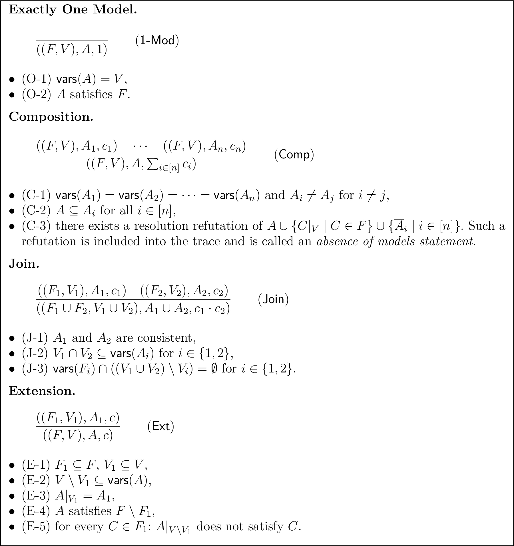
The rules of $\mathsf{MICE}$ are Exactly One Model (1-Mod), Composition (Comp), Join (Join) and Extension (Ext). They are specified in Fig. 1. We give some intuition on the rules. The axiom rule (1-Mod) states that if a complete assignment A satisfies a formula F, then F has exactly one model under A.

Figure 1.

Inference rules for $\mathsf{MICE}$ [24].

With (Comp) we can sum up model counts of a formula F under different partial assignments $A_1,\dots ,A_n$ in order to weaken the assumption to a partial assignment A. This is only sound if the solutions of F under assumptions $A_1,\dots ,A_n$ form a disjoint partition of the full solution space of F under A. That this is indeed the case can be verified with an independent proof, e.g. in propositional resolution. This proof is called an absence of models statement. We want to emphasize that the rule (Comp) can be applied with $n=0$ , i.e. we can derive any claim $((F,V),A,0)$ if $A\mathbf{\cup }\{C{|}_V\mid C\in F\}$ is unsatisfiable. In particular, we can derive $((\mathrm{\phi },\mathsf{vars}(\mathrm{\phi })),\varnothing ,0)$ for any unsatisfiable formula φ with a single application of (Comp).

The (Join) rule allows us to multiply the model counts of two formulas that are completely independent restricted to the assumptions. Finally, with (Ext), we can extend simultaneously all models, i.e. we enlarge the formula and assumption without changing the count.

We can now formally define $\mathsf{MICE}$ proofs.

Definition 3.2 (Fichte, Hecher, Roland [24]).

A $\mathsf{MICE}$ trace is a sequence $\mathrm{\pi }=(I_1,\dots ,I_k)$ where for each $i\in [k]$ , either

$I_i$ is a claim if $I_i$ is derived by one of (1-Mod), (Join), (Ext) or

$I_i=(I,\mathrm{\rho })$ if the claim I is derived by (Comp) and ρ is the resolution refutation for the respective absence of models statement.

A $\mathsf{MICE}$ proof of a formula φ is a $\mathsf{MICE}$ trace $\mathrm{\pi }=(I_1,\dots ,I_k)$ where $I_k$ is (or contains in case of (Comp)) the claim $((\mathrm{\phi },\mathsf{vars}(\mathrm{\phi })),\varnothing ,c)$ for some $c\in \mathbb{N}$ .

In [24] it is shown that $\mathsf{MICE}$ is a sound and complete proof system for #SAT.

For measuring the proof size, we use two natural options. $s(\mathrm{\pi })$ notates the size of π which is the total number of claims plus the number of clauses in resolution proofs in the absence of models statements. $c(\mathrm{\pi })$ counts only the number of claims a proof has which is exactly the number of inference steps that the proof needs.

In a correct claim $((F,V),A,c)$ the count c is uniquely determined by the formula F, set of variables V and assumption A. Therefore, we often omit c and refer to the claim as $((F,V),A)$ . To ease notation we will usually just write a $\mathsf{MICE}$ proof as sequence of claims $I_1,\dots ,I_m$ and do not explicitly record the used absence of models statements. We just assume that whenever we use (Comp), the necessary resolution refutation is part of the $\mathsf{MICE}$ proof.

If a formula F is satisfied by the partial assignment A, we can set the remaining variables arbitrarily. Therefore, the component $(F,\mathsf{vars}(F))$ has exactly $2^{|\mathsf{vars}(F)|\mathbf{-}|\mathsf{vars}(A)|}$ models under assumption A. The following construction shows that we can efficiently derive the corresponding claim in $\mathsf{MICE}$ .

Proposition 3.3.

If some assumption A satisfies an arbitrary formula F with $\mathsf{vars}(A)\subseteq \mathsf{vars}(F)$ , there is a $\mathsf{MICE}$ derivation of the claim $I=((F,\mathsf{vars}(F)),A,2^{|\mathsf{vars}(F)\mathbf{\setminus }\mathsf{vars}(A)|})$ with $s(\mathrm{\pi })=7\mathbf{\cdot }(|\mathsf{vars}(F)\mathbf{\setminus }\mathsf{vars}(A)|)$ and $c(\mathrm{\pi })=4\mathbf{\cdot }(|\mathsf{vars}(F)\mathbf{\setminus }\mathsf{vars}(A)|)$ .

Proof:

Let $\mathsf{vars}(F)\mathbf{\setminus }\mathsf{vars}(A)=\{x_1,\dots ,x_n\}$ . For every $i\in [n]$ we derive $I_i^1=((\varnothing ,\mathsf{vars}(A)\mathbf{\cup }\{x_i\}),A\mathbf{\cup }\{x_i\},1)$ and $I_i^0=((\varnothing ,\mathsf{vars}(A)\mathbf{\cup }\{x_i\}),A\mathbf{\cup }\{{\bar{x}}_i\},1)$ with (1-Mod). This is possible since every assignment satisfies the empty formula. With (Comp) we get $I_i=((\varnothing ,\mathsf{vars}(A)\mathbf{\cup }\{x_i\}),A,2)$ using the absence of models statement ${\mathrm{\rho }}_i=((x_i),({\bar{x}}_i),\square )$ . We use (Join) of $I_1$ and $I_2$ , then (Join) of the result and $I_3$ , and so on. The requirements (J-1), (J-2) and (J-3) are satisfied. In this way we get $((\varnothing ,\mathsf{vars}(F)),A,2^{|\mathsf{vars}(F)\mathbf{\setminus }\mathsf{vars}(A)|})$ . We use (Ext) to obtain $I=((F,\mathsf{vars}(F)),A,2^{|\mathsf{vars}(F)\mathbf{\setminus }\mathsf{vars}(A)|})$ . It is easy to see that all requirements (E-1) to (E-5) are satisfied. For (E-4), we use that A satisfies F. In total we use $4n$ $\mathsf{MICE}$ steps to derive I and we have n absence of models statements with 3 clauses each. □

We investigate some properties that any claim in a $\mathsf{MICE}$ proof has to fulfill. We assume that any $\mathsf{MICE}$ proof has no redundant claims, i.e. in the corresponding proof dag, there is a path from any node to the final claim. We also observe that for all inference rules, the derived F and V never shrink. This leads to the following two observations:

Observation 3.4.

If $((F,V),A)$ is derived from $((F_1,V_1),A_1)$ in a $\mathsf{MICE}$ trace (not necessarily in one step), then $F_1\subseteq F$ and $V_1\subseteq V$ .

Therefore, any claim $((F,V),A)$ in a $\mathsf{MICE}$ proof of φ fulfills $F\subseteq \mathrm{\phi }$ and $V\subseteq \mathsf{vars}(\mathrm{\phi })$ .

From Definition 3.1 it is not obvious how F and V are related. Intuitively, one might be tempted to set $V=\mathsf{vars}(F)$ for any claim $((F,V),A)$ . However, this would make the proof system exponentially weaker as we will see later. Lemma 3.6 will show that we can at least assume $\mathsf{vars}(F)\subseteq V$ for every claim. To show this we need the following lemma:

Lemma 3.5.

For any claim $((F,V),A)$ and any variable x, if $x\in \mathsf{vars}(F)\mathbf{\setminus }V$ , then literals x and $\bar{x}$ cannot both occur in F.

Proof:

Suppose there exists such an x. Since $((F,V),A)$ is not redundant, there is a path to the final claim. Thus, there have to be claims $((F_1,V_1),A_1)$ and $((F_2,V_2),A_2)$ directly adjacent in the path with $F\subseteq F_1\subseteq F_2$ , $V\subseteq V_1\subseteq V_2$ and $x\notin V_1$ , $x\in V_2$ . Now $((F_2,V_2),A_2)$ is directly derived from $((F_1,V_1),A_1)$ in one step. We argue that this is not possible:

It is impossible with (1-Mod), since this rule uses no previous claim.

It is impossible with (Comp), since $V_1\ne V_2$ .

It is impossible with (Join). Assume otherwise that $((F_1,V_1),A_1)$ is joined with some $((F_3,V_3),A_3)$ . Because of $x\in V_2=V_1\mathbf{\cup }{V}_3$ we have $x\in V_3$ . Then $x\in \mathsf{vars}(F_1)\mathbf{\cap }(V_3\mathbf{\setminus }{V}_1)$ , contradicting condition (J-3).

It is impossible with (Ext). Otherwise x has to be in $\mathsf{vars}(A_2)$ because of (E-2) and $x\in V_2\mathbf{\setminus }{V}_1$ per construction. Then $A_2{|}_{V_2\mathbf{\setminus }{V}_1}$ satisfies a clause in $F_1$ since both literals x and $\bar{x}$ occur in $F_1$ (because $F\subseteq F_1$ ). Thus condition (E-5) fails.

This leads to a contradiction. As a result, such an x can not exist. □

Lemma 3.6.

Let a formula φ and a $\mathsf{MICE}$ proof π for φ be given. Then there is a $\mathsf{MICE}$ proof ${\mathrm{\pi }}^{\prime }$ satisfying $\mathsf{vars}(F)\subseteq V$ for any claim $((F,V),A)\in {\mathrm{\pi }}^{\prime }$ such that $s({\mathrm{\pi }}^{\prime })=O(s{(\mathrm{\pi })}^3)$ and $c({\mathrm{\pi }}^{\prime })=c(\mathrm{\pi })$ .

Proof:

Let $\mathrm{\pi }=(I_1,\dots ,I_m)$ with $I_i=((F_i,V_i),A_i)$ . Because of Lemma 3.5, for any $i\in [m]$ , we can assume that there is no variable $x\in \mathsf{vars}(F_i)\mathbf{\setminus }{V}_i$ that occurs in both polarities in $F_i$ . Let ${\mathrm{\alpha }}_i\in ⟨\mathsf{vars}(F_i)\mathbf{\setminus }{V}_i⟩$ be the assignment that does not satisfy any clause in $F_i$ , i.e. if x is in $F_i$ we assign ${\mathrm{\alpha }}_i(x)=0$ and vice versa. For every claim $I_i$ , ${\mathrm{\alpha }}_i$ exists and it is unique. We define $$\begin{array}{c}f\left(\right((F_i,V_i),A_i\left)\right):=\left(\right(F_i,V_i\mathbf{\cup }\mathsf{vars}(F_i)),A_i\mathbf{\cup }{\mathrm{\alpha }}_i)\end{array}$$ with the unique ${\mathrm{\alpha }}_i$ defined above. Note that $A_i$ and ${\mathrm{\alpha }}_i$ have no variables in common and are therefore consistent. The resulting claim on the right side satisfies the requirement we want to achieve.

We show by induction that $(f(I_1),\dots ,f(I_k))$ is a valid $\mathsf{MICE}$ trace for all $k\in \{0,\dots ,m\}$ . In the base case $k=0$ the empty trace is valid. For the induction step we assume that we have already derived $f(I_1),\dots ,f(I_{k\mathbf{-}1})$ . In particular, we have derived $f(I)$ for every claim I we used to derive $I_k$ . We consider the different rules from which $I_k$ could be derived.

Exactly One Model.  $I_k=((F_k,V_k),A_k)$ is derived with (1-Mod). We can derive $f(I_k)=((F_k,V_k\mathbf{\cup }\mathsf{vars}(F_k)),A_k\mathbf{\cup }{\mathrm{\alpha }}_k)$ with (1-Mod) as well.

(O-1). $\mathsf{vars}(A_k\mathbf{\cup }{\mathrm{\alpha }}_k)=V_k\mathbf{\cup }\mathsf{vars}(F_k)$ since $\mathsf{vars}(A_k)=V_k$ ((O-1) for $I_k$ ) and $\mathsf{vars}({\mathrm{\alpha }}_k)=\mathsf{vars}(F_k)\mathbf{\setminus }{V}_k$ .

(O-2). $A_k\mathbf{\cup }{\mathrm{\alpha }}_k$ satisfies $F_k$ , since $A_k$ satisfies $F_k$ ((O-2) for $I_k$ ).

Composition.  $I_k=((F_k,V_k),A_k)$ is derived with (Comp) of claims $I_{i_1},\dots ,I_{i_r}$ with $i_j<k$ and $I_{i_j}=((F_k,V_k),A_{i_j})$ for $j\in [r]$ . Let ρ be the absence of models statement ((C-3) for $I_k$ ) that refutes $$\begin{array}{c}\{C{|}_{V_k}\mid C\in F_k\}\mathbf{\cup }{A}_k\mathbf{\cup }\{{\bar{A}}_{i_j}\mid j\in [r]\}.\end{array}$$ For $j\in [r]$ let $f(I_{i_j})=((F_k,V_k\mathbf{\cup }\mathsf{vars}(F_k)),A_{i_j}\mathbf{\cup }{\mathrm{\alpha }}_k)$ with ${\mathrm{\alpha }}_k={\mathrm{\alpha }}_{i_j}$ , since ${\mathrm{\alpha }}_{i_j}$ does only depend on $F_k$ and $V_k$ and is therefore equal to ${\mathrm{\alpha }}_k$ . To derive $f(I_k)=((F_k,V_k\mathbf{\cup }\mathsf{vars}(F_k)),A_k\mathbf{\cup }{\mathrm{\alpha }}_k)$ we can use (Comp) of $f(I_{i_1}),\dots ,f(I_{i_r})$ :

(C-1). $A_{i_j}\mathbf{\cup }{\mathrm{\alpha }}_k$ assign the same variables and are pairwise inconsistent, since $A_{i_j}$ assign the same variables and are pairwise inconsistent ((C-1) for $I_k$ ).

(C-2). For every $j\in [r]$ we have $A_k\subseteq A_{i_j}$ ((C-2) for $I_k$ ) and in particular $A_k\mathbf{\cup }{\mathrm{\alpha }}_k\subseteq A_{i_j}\mathbf{\cup }{\mathrm{\alpha }}_k$ .

(C-3). We need an absence of models statement that refutes $$\begin{array}{rl}& \{C{|}_{V_k\mathbf{\cup }\mathsf{vars}(F_k)}\mid C\in F_k\}\mathbf{\cup }(A_k\mathbf{\cup }{\mathrm{\alpha }}_k)\mathbf{\cup }\{\overline{A_{i_j}\mathbf{\cup }{\mathrm{\alpha }}_k}\mid j\in [r]\}\\ & =F_k\mathbf{\cup }{A}_k\mathbf{\cup }{\mathrm{\alpha }}_k\mathbf{\cup }\{({\bar{A}}_{i_j}\mathbf{\vee }{\bar{\mathrm{\alpha }}}_k)\mid j\in [r]\}\end{array}$$ For this we do at most $(|F_k|\mathbf{+}r)\mathbf{\cdot }|{\mathrm{\alpha }}_k|=O(|\mathrm{\pi }{|}^2)$ resolution steps to remove all ${\mathrm{\alpha }}_k$ literals from $F_k$ and $({\bar{A}}_{i_j}\mathbf{\vee }{\bar{\mathrm{\alpha }}}_k)$ . Note that this is possible, since for any $x\in \mathsf{lits}({\mathrm{\alpha }}_k)$ , only $\bar{x}$ can appear in $\mathsf{lits}(F_k)$ per construction of ${\mathrm{\alpha }}_k$ . It remains exactly the formula that is refuted by ρ as all variables from ${\mathrm{\alpha }}_k$ are removed.

Join.  $I_k=((F_k,V_k),A_k)=((F_i\mathbf{\cup }{F}_j,V_i\mathbf{\cup }{V}_j),A_i\mathbf{\cup }{A}_j)$ is derived using (Join) of claims $I_i=((F_i,V_i),A_i)$ and $I_j=((F_j,V_j),A_j)$ with $i,j<k$ . First, we show $$\begin{array}{c}\mathsf{vars}(F_i)\mathbf{\setminus }(V_i\mathbf{\cup }{V}_j)=\mathsf{vars}(F_i)\mathbf{\setminus }{V}_i.\end{array}$$

The inclusion ⊆ follows directly. To show the other direction ⊇, assume $x\in \mathsf{vars}(F_i)$ and $x\notin V_i$ . Because of (J-3) for $I_k$ is $x\notin \mathsf{vars}(F_i)\mathbf{\cap }(V_j\mathbf{\setminus }{V}_i)$ . Thus, $x\notin V_j$ and therefore, $x\in \mathsf{vars}(F_i)\mathbf{\setminus }(V_i\mathbf{\cup }{V}_j)$ .

Using this we can prove $$\begin{array}{c}{\mathrm{\alpha }}_k={\mathrm{\alpha }}_i\mathbf{\cup }{\mathrm{\alpha }}_j.\end{array}$$ For that it is sufficient to show that both sides assign the same variables and that they are consistent.

We show that $\mathsf{vars}({\mathrm{\alpha }}_k)=\mathsf{vars}({\mathrm{\alpha }}_i)\mathbf{\cup }\mathsf{vars}({\mathrm{\alpha }}_j)$ . With the definitions of α and $F_k$ we get $\mathsf{vars}({\mathrm{\alpha }}_k)=\mathsf{vars}(F_k)\mathbf{\setminus }{V}_k=\mathsf{vars}(F_i\mathbf{\cup }{F}_j)\mathbf{\setminus }(V_i\mathbf{\cup }{V}_j)$ . Applying simple set operations and the equation from above, this is equal to $(\mathsf{vars}(F_i)\mathbf{\setminus }(V_i\mathbf{\cup }{V}_j))\mathbf{\cup }(\mathsf{vars}(F_j)\mathbf{\setminus }(V_i\mathbf{\cup }{V}_j))=(\mathsf{vars}(F_i)\mathbf{\setminus }{V}_i)\mathbf{\cup }(\mathsf{vars}(F_j)\mathbf{\setminus }{V}_j)$ . This is exactly $\mathsf{vars}({\mathrm{\alpha }}_i)\mathbf{\cup }\mathsf{vars}({\mathrm{\alpha }}_j)$ per definition.

To show consistency of ${\mathrm{\alpha }}_i$ , ${\mathrm{\alpha }}_j$ and ${\mathrm{\alpha }}_k$ , we show that every pair is consistent. ${\mathrm{\alpha }}_i$ and ${\mathrm{\alpha }}_j$ are consistent: Otherwise suppose $x\in \mathsf{lits}({\mathrm{\alpha }}_i)$ and $\bar{x}\in \mathsf{lits}({\mathrm{\alpha }}_j)$ for some literal x. Per construction is $\bar{x}\in \mathsf{lits}(F_i)$ , $x\in \mathsf{lits}(F_j)$ and therefore, $x\in \mathsf{lits}(F_k)$ , $\bar{x}\in \mathsf{lits}(F_k)$ . Furthermore, $\mathsf{var}(x)\notin (V_i\mathbf{\cup }{V}_j)=V_k$ . As a result, $\mathsf{var}(x)\in \mathsf{vars}(F_k)\mathbf{\setminus }{V}_k$ and x occurs in both polarities in $F_k$ leading to a contradiction to Lemma 3.5. ${\mathrm{\alpha }}_k$ and ${\mathrm{\alpha }}_i$ are consistent: Assume $x\in \mathsf{vars}({\mathrm{\alpha }}_k)$ and $x\in \mathsf{vars}({\mathrm{\alpha }}_i)$ for some variable x. W.l.o.g. let $x\in \mathsf{lits}({\mathrm{\alpha }}_k)$ . Then, $\bar{x}\in \mathsf{lits}(F_k)=\mathsf{lits}(F_i\mathbf{\cup }{F}_j)$ leading to $\bar{x}\in \mathsf{lits}(F_i)$ and $x\in \mathsf{lits}({\mathrm{\alpha }}_i)$ . Analogously we get that ${\mathrm{\alpha }}_k$ and ${\mathrm{\alpha }}_j$ are consistent.

To derive $$\begin{array}{rl}f(I_k)& =\left(\right(F_k,V_k\mathbf{\cup }\mathsf{vars}(F_k)),A_k\mathbf{\cup }{\mathrm{\alpha }}_k)\\ & =\left(\right(F_i\mathbf{\cup }{F}_j,V_i\mathbf{\cup }{V}_j\mathbf{\cup }\mathsf{vars}(F_i)\mathbf{\cup }\mathsf{vars}(F_j)),A_i\mathbf{\cup }{A}_j\mathbf{\cup }{\mathrm{\alpha }}_i\mathbf{\cup }{\mathrm{\alpha }}_j)\end{array}$$ we can use (Join) of $f(I_i)=((F_i,V_i\mathbf{\cup }\mathsf{vars}(F_i)),A_i\mathbf{\cup }{\mathrm{\alpha }}_i)$ and $f(I_j)=((F_j,V_j\mathbf{\cup }\mathsf{vars}(F_j)),A_j\mathbf{\cup }{\mathrm{\alpha }}_j)$ :

(J-1). $A_i$ and $A_j$ are consistent because of (J-1) for $I_k$ . We showed already that ${\mathrm{\alpha }}_i$ and ${\mathrm{\alpha }}_j$ are consistent. $A_i$ and ${\mathrm{\alpha }}_j$ are consistent, because they have no variables in common. Otherwise let x be a variable with $x\in \mathsf{vars}(A_i)$ and $x\in \mathsf{vars}({\mathrm{\alpha }}_j)$ . Per construction is $x\in V_i$ , $x\in \mathsf{vars}(F_j)$ and $x\notin V_j$ and thus, $x\in \mathsf{vars}(F_j)\mathbf{\cap }(V_i\mathbf{\setminus }{V}_j)$ . This contradicts (J-3) for $I_k$ . The same argument shows that $A_j$ and ${\mathrm{\alpha }}_i$ are consistent.

As a result, $A_i\mathbf{\cup }{\mathrm{\alpha }}_i$ and $A_j\mathbf{\cup }{\mathrm{\alpha }}_j$ are consistent.

(J-2). First we show $$\begin{array}{c}{V}_i\mathbf{\cap }\mathsf{vars}({\mathrm{\alpha }}_j)=\varnothing \text{and}{V}_j\mathbf{\cap }\mathsf{vars}({\mathrm{\alpha }}_i)=\varnothing .\end{array}$$ For the sake of contradiction, assume there is a variable x with $x\in V_i$ and $x\in \mathsf{vars}({\mathrm{\alpha }}_j)$ . Per construction is $x\in \mathsf{vars}(F_j)$ and $x\notin V_j$ and thus $x\in \mathsf{vars}(F_j)\mathbf{\cap }(V_i\mathbf{\setminus }{V}_j)$ which contradicts (J-3) for $I_k$ . Analogously we get $V_j\mathbf{\cap }\mathsf{vars}({\mathrm{\alpha }}_i)=\varnothing$ . Furthermore, $(V_i\mathbf{\cap }{V}_j)\subseteq \mathsf{vars}(A_r)$ for $r\in \{i,j\}$ because of (J-2) for $I_k$ . Using this, we get $$\begin{array}{rl}& (V_i\mathbf{\cup }\mathsf{vars}({\mathrm{\alpha }}_i))\mathbf{\cap }(V_j\mathbf{\cup }\mathsf{vars}({\mathrm{\alpha }}_j))\\ & =(V_i\mathbf{\cap }{V}_j)\mathbf{\cup }(\mathsf{vars}({\mathrm{\alpha }}_i)\mathbf{\cap }\mathsf{vars}({\mathrm{\alpha }}_j))\mathbf{\cup }(V_i\mathbf{\cap }\mathsf{vars}({\mathrm{\alpha }}_j))\mathbf{\cup }(V_j\mathbf{\cap }\mathsf{vars}({\mathrm{\alpha }}_i))\\ & =(V_i\mathbf{\cap }{V}_j)\mathbf{\cup }(\mathsf{vars}({\mathrm{\alpha }}_i)\mathbf{\cap }\mathsf{vars}({\mathrm{\alpha }}_j))\\ & \subseteq \mathsf{vars}(A_r)\mathbf{\cup }(\mathsf{vars}({\mathrm{\alpha }}_i)\mathbf{\cap }\mathsf{vars}({\mathrm{\alpha }}_j))\\ & \subseteq \mathsf{vars}(A_r)\mathbf{\cup }\mathsf{vars}({\mathrm{\alpha }}_r)\end{array}$$ for $r\in \{i,j\}$ .

(J-3). The requirement $\mathsf{vars}(F_i)\mathbf{\cap }((V_i\mathbf{\cup }{V}_j)\mathbf{\setminus }{V}_i)=\varnothing$ is always fulfilled if the two joined claims satisfy $\mathsf{vars}(F_i)\subseteq V_i$ .

Extension.  $I_k=((F_k,V_k),A_k)$ is derived using (Ext) of $I_i=((F_i,V_i),A_i)$ with $i<k$ . Then we can also derive $f(I_k)=((F_k,V_k\mathbf{\cup }\mathsf{vars}(F_k)),A_k\mathbf{\cup }{\mathrm{\alpha }}_k)$ from $f(I_i)=((F_i,V_i\mathbf{\cup }\mathsf{vars}(F_i)),A_i\mathbf{\cup }{\mathrm{\alpha }}_i)$ with (Ext):

(E-1). $F_i\subseteq F_k$ , $V_i\mathbf{\cup }\mathsf{vars}(F_i)\subseteq V_k\mathbf{\cup }\mathsf{vars}(F_k)$ is fulfilled, since $F_i\subseteq F_k$ and $V_i\subseteq V_k$ because of (E-1) for $I_k$ .

(E-2). We have to show $(V_k\mathbf{\cup }\mathsf{vars}(F_k))\mathbf{\setminus }(V_i\mathbf{\cup }\mathsf{vars}(F_i))\subseteq \mathsf{vars}(A_k\mathbf{\cup }{\mathrm{\alpha }}_k)$ . For this, let x be an arbitrary variable with $x\in (V_k\mathbf{\cup }\mathsf{vars}(F_k))\mathbf{\setminus }(V_i\mathbf{\cup }\mathsf{vars}(F_i))$ . If $x\in V_k$ , then $x\in V_k\mathbf{\setminus }{V}_i\subseteq \mathsf{vars}(A_k)$ because of (E-2) for $I_k$ . Otherwise if $x\notin V_k$ , $x\in \mathsf{vars}(F_k)$ and thus $x\in \mathsf{vars}({\mathrm{\alpha }}_k)$ per construction of ${\mathrm{\alpha }}_k$ .

(E-3). We have to show that $(A_k\mathbf{\cup }{\mathrm{\alpha }}_k){|}_{V_i\mathbf{\cup }\mathsf{vars}(F_i)}=A_i\mathbf{\cup }{\mathrm{\alpha }}_i$ . For this we use $$\begin{array}{c}{A}_k{|}_{V_i}=A_i\end{array}$$ which follows from (E-3) for $I_k$ . Furthermore, by using $V_i\subseteq V_k$ and $\mathsf{vars}(\mathrm{\alpha })\mathbf{\cap }{V}_k=\varnothing$ , we receive $$\begin{array}{c}{\mathrm{\alpha }}_k{|}_{V_i}={\mathrm{\alpha }}_k{|}_{V_k\mathbf{\cap }{V}_i}=({\mathrm{\alpha }}_k{|}_{V_k}){|}_{V_i}=\varnothing .\end{array}$$ Next, we prove $$\begin{array}{c}(A_k\mathbf{\cup }{\mathrm{\alpha }}_k){|}_{\mathsf{vars}(F_i)\mathbf{\setminus }{V}_i}={\mathrm{\alpha }}_i.\end{array}$$ For this we show that both assign the same variables and then that every variable is assigned equally.

To show that both sides assign the same variables, the direction ⊆ follows with $\mathsf{vars}((A_k\mathbf{\cup }{\mathrm{\alpha }}_k){|}_{\mathsf{vars}(F_i)\mathbf{\setminus }{V}_i})\subseteq \mathsf{vars}(F_i)\mathbf{\setminus }{V}_i=\mathsf{vars}({\mathrm{\alpha }}_i)$ . For the other direction ⊇, let $x\in \mathsf{vars}({\mathrm{\alpha }}_i)$ implying $x\in \mathsf{vars}(F_i)\mathbf{\setminus }{V}_i$ . Thus, we have to show that $x\in \mathsf{vars}(A_k\mathbf{\cup }{\mathrm{\alpha }}_k)$ . If $x\in V_k$ , then $x\in V_k\mathbf{\setminus }{V}_i$ and thus, $x\in \mathsf{vars}(A_k)$ because of (E-2) for $I_k$ . If $x\notin V_k$ , then $x\in {\mathrm{\alpha }}_k$ , since $x\in \mathsf{vars}(F_i)\subseteq \mathsf{vars}(F_k)$ .

In order to show that ${\mathrm{\alpha }}_k$ and ${\mathrm{\alpha }}_i$ are consistent, assume $x\in \mathsf{vars}({\mathrm{\alpha }}_k)\mathbf{\cap }\mathsf{vars}({\mathrm{\alpha }}_i)$ and let $x\in \mathsf{lits}({\mathrm{\alpha }}_i)$ . Then we have $\bar{x}\in \mathsf{lits}(F_i)\subseteq \mathsf{lits}(F_k)$ leading to $x\in \mathsf{lits}({\mathrm{\alpha }}_k)$ . $A_k$ , ${\mathrm{\alpha }}_i$ are consistent: Assume $x\in \mathsf{vars}(A_k)\mathbf{\cap }\mathsf{vars}({\mathrm{\alpha }}_i)$ and let $x\in \mathsf{lits}({\mathrm{\alpha }}_i)$ . Then $\bar{x}\in \mathsf{lits}(F_i)$ , $x\notin V_i$ , $x\in V_k$ . Because of (E-5) for $I_k$ , $A_k{|}_{V_k\mathbf{\setminus }{V}_i}$ and in particular $A_k{|}_{\{x\}}$ does not satisfy any $C\in F_i$ . Since there is a clause in $F_i$ that contains literal $\bar{x}$ , $x\in \mathsf{lits}(A_k)$ .

Using those three properties from above we get $$\begin{array}{c}(A_k\mathbf{\cup }{\mathrm{\alpha }}_k){|}_{V_i\mathbf{\cup }\mathsf{vars}(F_i)}=A_k{|}_{V_i}\mathbf{\cup }{\mathrm{\alpha }}_k{|}_{V_i}\mathbf{\cup }(A_k\mathbf{\cup }{\mathrm{\alpha }}_k){|}_{\mathsf{vars}(F_i)\mathbf{\setminus }{V}_i}=A_i\mathbf{\cup }{\mathrm{\alpha }}_i.\end{array}$$

(E-4). $(A_k\mathbf{\cup }{\mathrm{\alpha }}_k)$ satisfies $F_k\mathbf{\setminus }{F}_i$ , since $A_k$ satisfies $F_k\mathbf{\setminus }{F}_i$ (E-4) for $I_k$ .

(E-5). $(A_k\mathbf{\cup }{\mathrm{\alpha }}_k){|}_{(V_k\mathbf{\cup }\mathsf{vars}(F_k))\mathbf{\setminus }(V_i\mathbf{\cup }\mathsf{vars}(F_i))}$ does not satisfy C for any $C\in F_i$ as the restricted assignment has no variables in $\mathsf{vars}(F_i)$ .

This completes the induction. Since $I_m=((\mathrm{\phi },\mathsf{vars}(\mathrm{\phi })),\varnothing )=f(I_m)$ , ${\mathrm{\pi }}^{\prime }=(f(I_1),\dots ,f(I_m))$ is a valid proof for φ with the claimed property. The number of claims does not change. The number of clauses in the refutation does only increase in the (Comp) case and at most by a factor of $O(s{(\mathrm{\pi })}^2)$ . □

In the following we always assume $\mathsf{vars}(F)\subseteq V$ for any claim $((F,V),A)$ . With this requirement, the conditions of the inference rules can be simplified.

Corollary 3.7.

If we require $\mathsf{vars}(F)\subseteq V$ for every claim $((F,V),A)$ , the following simplifications for the $\mathsf{MICE}$ rules apply:

We can simplify the absence of models statement in the requirement (C-3) to be a refutation of $F\mathbf{\cup }A\mathbf{\cup }\{\overline{A_i}\mid i\in [n]\}$ .

We can remove condition (J-3) for (Join).

We can remove condition (E-5) for (Ext).

However, imposing the stronger condition $\mathsf{vars}(F)=V$ for every claim $((F,V),A)$ would make the proof system exponentially weaker as we illustrate with the next proposition.

Lemma 3.8.

There is a family of formulas ${(T_n)}_{n\in \mathbb{N}}$ such that for both measures $s(\mathbf{\cdot })$ and $c(\mathbf{\cdot })$ holds:

$T_n$ has polynomial-size $\mathsf{MICE}$ proofs and

if $\mathsf{vars}(F)=V$ is required for all claims $((F,V),A)$ , the shortest $\mathsf{MICE}$ proof of $T_n$ has exponential size.

Proof:

Consider the family of formulas ${(T_n)}_{n\in \mathbb{N}}$ that only have one clause $$\begin{array}{c}(x_1\mathbf{\vee }{x}_2\mathbf{\vee }\cdots \mathbf{\vee }{x}_n).\end{array}$$ First we show that $T_n$ has a $\mathsf{MICE}$ proof of size $O(n^2)$ for every n. With the construction of Proposition 3.3 we derive $$\begin{array}{rl}& I_1=\left(\right(T_n,\mathsf{vars}(T_n)),\{x_1=1\},2^{n\mathbf{-}1}),\\ & I_2=\left(\right(T_n,\mathsf{vars}(T_n)),\{x_1=0,x_2=1\},2^{n\mathbf{-}2}),\\ & ⋮\\ & I_n=\left(\right(T_n,\mathsf{vars}(T_n)),\{x_1=0,x_2=0,\dots ,x_{n\mathbf{-}1}=0,x_n=1\},1).\end{array}$$ We apply (Comp) to the one claim $I_n$ which results in $$\begin{array}{c}{J}_n=\left(\right(T_n,\mathsf{vars}(T_n)),\{x_1=0,x_2=0,\dots ,x_{n\mathbf{-}1}=0\},1).\end{array}$$ Then, we use (Comp) of $J_n$ and $I_{n\mathbf{-}1}$ which results in $$\begin{array}{c}{J}_{n\mathbf{-}1}=\left(\right(T_n,\mathsf{vars}(T_n)),\{x_1=0,x_2=0,\dots ,x_{n\mathbf{-}2}=0\},3).\end{array}$$ Similarly we apply (Comp) to every pair of claims $I_i$ and $J_{i\mathbf{+}1}$ and finally get $$\begin{array}{c}{J}_1=\left(\right(T_n,\mathsf{vars}(T_n)),\varnothing ,2^n\mathbf{-}1).\end{array}$$ In total we need $O(n^2)$ steps to derive all $I_i$ and n applications of (Comp) to combine these claims.

Next, we show that any $\mathsf{MICE}$ proof with the additional requirement $\mathsf{vars}(F)=V$ has size $2^{\Omega (n)}$ . Note that the construction from Proposition 3.3 does not work under this additional requirement.

We show that the claim $I_{\varnothing }=((\varnothing ,\varnothing ),\varnothing ,1)$ does not help for the proof. If we use (Join) on $I_{\varnothing }$ together with any claim I, the result is I. Similarly, if we derive I with (Ext) from $I_{\varnothing }$ , we can derive I with (1-Mod) without $I_{\varnothing }$ . If we apply (Comp) on claim $I_{\varnothing }$ together with some other claims, (C-1) implies that all used claims have to be $I_{\varnothing }$ . Thus, (Comp) would result in $I_{\varnothing }$ . Therefore, we can assume $I_{\varnothing }$ is not in the proof at all.

Thus, the only component we can use is $C=(\{x_1\mathbf{\vee }\dots \mathbf{\vee }{x}_n\},\{x_1,\dots ,x_n\})$ . Assume I is derived with (Join) from $I_1=(C,A_1)$ and $I_2=(C,A_2)$ . Condition (J-2) implies $\mathsf{vars}(A_1)=\mathsf{vars}(A_2)=\{x_1,\dots ,x_n\}$ and in particular $A_1=A_2$ because of (J-1). Therefore, $I=I_1=I_2$ and the usage of (Join) is redundant. Let $I=(C,A)$ be derived from $I_1=(C,A_1)$ with (Ext). Because of (E-3) we have $A=A_1$ and hence $I=I_1$ . Hence, the rules (Join) and (Ext) achieve nothing and we can assume that they do not appear in the proof.

As a result, the proof can only use rules (1-Mod) and (Comp). Such a proof needs $2^n\mathbf{-}1$ applications of (1-Mod) as $T_n$ has $2^n\mathbf{-}1$ models. □

4. A Simplified Proof System MICE’ for #SAT

We now adapt $\mathsf{MICE}$ to a new proof system $\mathsf{MIC}{E}^{\prime }$ that is as strong as $\mathsf{MICE}$ and only uses claims $((F,V),A)$ with components satisfying $V=\mathsf{vars}(F)$ . Therefore, we can drop the explicit mentioning of the variable set V and only need to specify the formula F. This makes the resulting proof system more intuitive and easier to investigate for lower bounds.

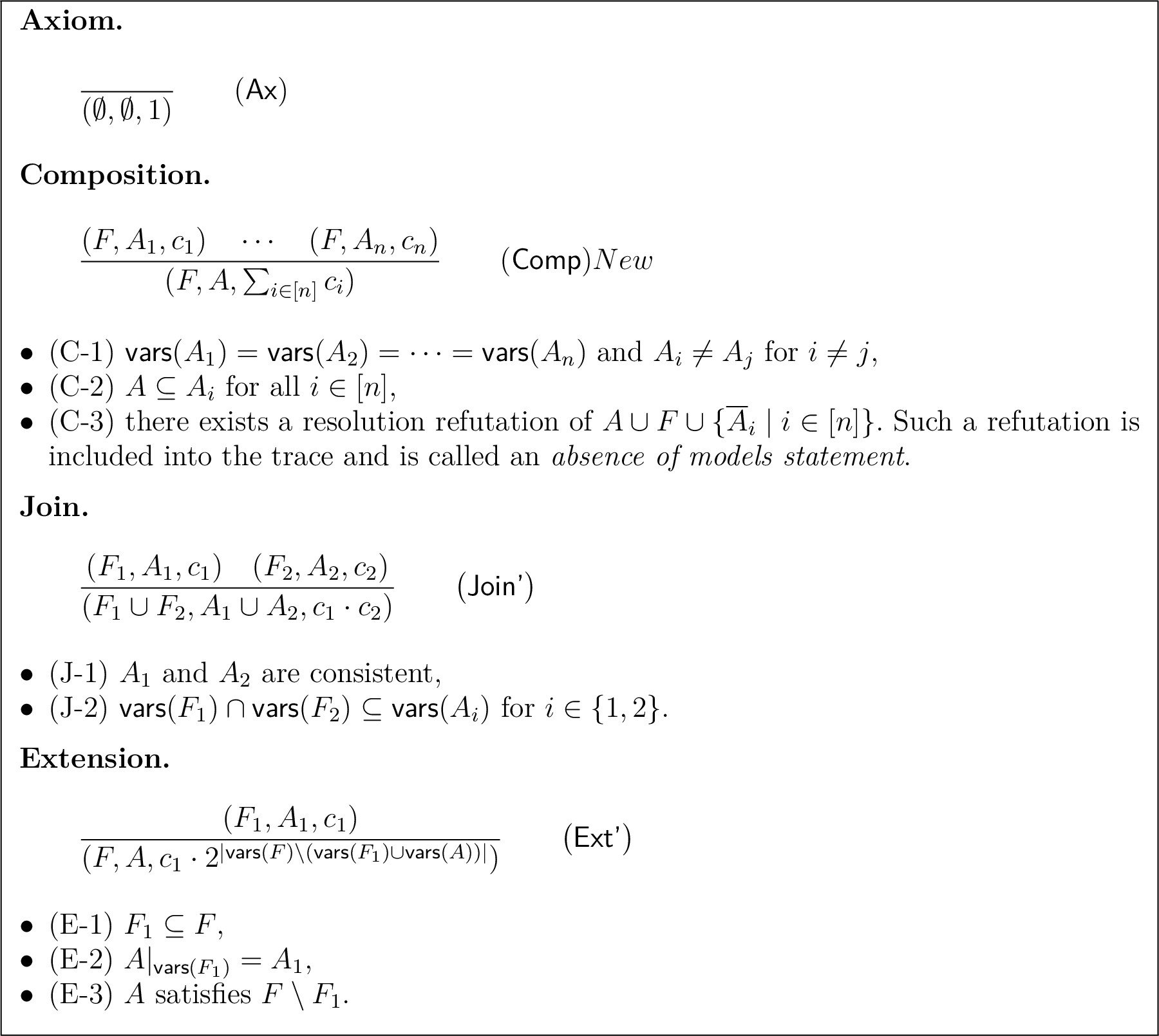
The rules of $\mathsf{MIC}{E}^{\prime }$ are Axiom (Ax), Composition (Comp’), Join (Join’) and Extension (Ext’). They are specified in Fig. 2.

Figure 2.

Inference rules for $\mathsf{MIC}{E}^{\prime }$ .

The intuition for the rules (Comp’) and (Join’) are very similar to (Comp) and (Join) from $\mathsf{MICE}$ . The (Ax) rule enables us to derive the claim $(\varnothing ,\varnothing ,1)$ which is trivially true. (Ext’) is also similar to (Ext) with one important difference: If we use (Ext) in $\mathsf{MICE}$ , the assumption has to assign all variables that are added to the claim. As a result, we extend one model of the original claim to one new model. In (Ext’) however, this is not necessarily the case. As long as the new assumption satisfies all added clauses, we are allowed to leave new introduced variables unassigned in the assumption. Like this we extend every model of the original claim to a set of new models, one for every possible assignment of these unassigned variables.

Definition 4.1 (Adapted Proof System $\mathsf{MIC}{E}^{\prime }$ ).

A claim is a triple $(F,A,c)$ with $\mathsf{vars}(A)\subseteq \mathsf{vars}(F)$ . For such a claim, let ${\mathsf{Mod}}_A(F):=\{\mathrm{\alpha }\in ⟨\mathsf{vars}(F)⟩\mid \mathrm{\alpha }\vDash F\mathbf{\cup }A\}$ . The claim is correct if $c=|{\mathsf{Mod}}_A(F)|$ . The rules of $\mathsf{MIC}{E}^{\prime }$ are (Ax), (Comp’), (Join’) and (Ext’). The notions of $\mathsf{MIC}{E}^{\prime }$ traces and $\mathsf{MIC}{E}^{\prime }$ proofs are defined analogously as for $\mathsf{MICE}$ . Furthermore, we use the same two measures for the proof size $s(\mathbf{\cdot })$ and $c(\mathbf{\cdot })$ .

As in the $\mathsf{MICE}$ proof system we often omit the count c of claims and assume that no redundant claims exist in $\mathsf{MIC}{E}^{\prime }$ proofs, i.e. all claims are connected to the final claim.

We prove that all four derivation rules are sound, i.e. for every derived claim $(F,A,c)$ holds $c=|{\mathsf{Mod}}_A(F)|$ . In doing so, we will also provide some intuition on the semantic meaning of the rules.

Lemma 4.2.

The inference rules of $\mathsf{MIC}{E}^{\prime }$ are sound.

Proof:

To prove the soundness of every $\mathsf{MIC}{E}^{\prime }$ rule, we associate every claim $(F,A,c)$ with the set ${\mathsf{Mod}}_A(F)$ . With this interpretation, we can specify how every rule modifies these models. This way, we can show that the resulting model count is indeed correct for every $\mathsf{MIC}{E}^{\prime }$ rule.

The soundness of (Ax) is obvious, since $|{\mathsf{Mod}}_{\varnothing }(\varnothing )|=|\{\varnothing \}|=1$ .

To show soundness of (Comp’), let $(F,A,{\sum }_{i\in [n]}{c}_i)$ be derived with (Comp’) from correct claims $(F,A_1,c_1),\dots ,(F,A_n,c_n)$ . Then we have $$\begin{array}{rl}& {\mathsf{Mod}}_A(F)\\ & =\{\mathrm{\alpha }\in ⟨\mathsf{vars}(F)⟩\mid \mathrm{\alpha }\vDash F\mathbf{\cup }A\}\\ & =\underset{i\in [n]}{{\displaystyle \uplus }}\{\mathrm{\alpha }\in ⟨\mathsf{vars}(F)⟩\mid \mathrm{\alpha }\vDash F\mathbf{\cup }{A}_i\}\mathbf{\uplus }\{\mathrm{\alpha }\in ⟨\mathsf{vars}(F)⟩\mid \mathrm{\alpha }\vDash F\mathbf{\cup }A\mathbf{\cup }\{{\bar{A}}_i\mid i\in [n]\left\}\right\}\end{array}$$ where ⊎ denotes the disjoint union. This split of A into those $A_i$ is possible since $A\subseteq A_i$ (C-2). The sets on the right side of the equation are pairwise disjoint because of (C-1). The last set is empty, otherwise there would not exist an absence of models statement (C-3). Thus, $$\begin{array}{c}{\mathsf{Mod}}_A(F)=\underset{i\in [n]}{{\displaystyle \uplus }}{\mathsf{Mod}}_{A_i}(F).\end{array}$$ Using the correctness of all used claims we get $$\begin{array}{c}|{\mathsf{Mod}}_A(F)|={\displaystyle \sum }_{i\in [n]}|{\mathsf{Mod}}_{A_i}(F)|={\displaystyle \sum }_{i\in [n]}{c}_i.\end{array}$$ Next, we show soundness of (Join’). For this, let $(F_1\mathbf{\cup }{F}_2,A_1\mathbf{\cup }{A}_2,c_1\mathbf{\cdot }{c}_2)$ be derived with (Join’) from correct claims $(F_1,A_1,c_1)$ and $(F_2,A_2,c_2)$ . We show that $$\begin{array}{c}{\mathsf{Mod}}_{A_1\mathbf{\cup }{A}_2}(F_1\mathbf{\cup }{F}_2)=\{{\mathrm{\alpha }}_1\mathbf{\cup }{\mathrm{\alpha }}_2\mid {\mathrm{\alpha }}_1\in {\mathsf{Mod}}_{A_1}(F_1),{\mathrm{\alpha }}_2\in {\mathsf{Mod}}_{A_2}(F_2)\}.\end{array}$$ We will prove both subset relations separately in the following.

For ⊆, let $\mathrm{\alpha }\in {\mathsf{Mod}}_{A_1\mathbf{\cup }{A}_2}(F_1\mathbf{\cup }{F}_2)$ be given. Per definition, α satisfies $F_1\mathbf{\cup }{F}_2\mathbf{\cup }{A}_1\mathbf{\cup }{A}_2$ and in particular $\mathrm{\alpha }{|}_{\mathsf{vars}(F_1)\mathbf{\cup }\mathsf{vars}(A_1)}$ has to satisfy $F_1\mathbf{\cup }{A}_1$ . Because of $\mathsf{vars}(A_1)\subseteq \mathsf{vars}(F_1)$ , $\mathrm{\alpha }{|}_{\mathsf{vars}(F_1)}$ has to satisfy $F_1\mathbf{\cup }{A}_1$ and therefore, $\mathrm{\alpha }{|}_{\mathsf{vars}(F_1)}\in {\mathsf{Mod}}_{A_1}(F_1)$ . Analogously, we get $\mathrm{\alpha }{|}_{\mathsf{vars}(F_2)}\in {\mathsf{Mod}}_{A_2}(F_2)$ . Since $\mathrm{\alpha }=\mathrm{\alpha }{|}_{\mathsf{vars}(F_1)}\mathbf{\cup }\mathrm{\alpha }{|}_{\mathsf{vars}(F_2)}$ , we can choose ${\mathrm{\alpha }}_1=\mathrm{\alpha }{|}_{\mathsf{vars}(F_1)}$ and ${\mathrm{\alpha }}_2=\mathrm{\alpha }{|}_{\mathsf{vars}(F_2)}$ to see the relation.

For the other direction ⊇, we first have to show that any fixed ${\mathrm{\alpha }}_1\in {\mathsf{Mod}}_{A_1}(F_1)$ and ${\mathrm{\alpha }}_2\in {\mathsf{Mod}}_{A_2}(F_2)$ are consistent. Because of (J-2) ensuring $\mathsf{vars}(F_1)\mathbf{\cap }\mathsf{vars}(F_2)\subseteq \mathsf{vars}(A_i)$ for both $i\in \{1,2\}$ , we know that they could only be inconsistent in variables in $A_i$ . With (J-1) which states that $A_1$ and $A_2$ are consistent, we can conclude that ${\mathrm{\alpha }}_1$ and ${\mathrm{\alpha }}_2$ are consistent. We know that ${\mathrm{\alpha }}_i$ satisfies $F_i\mathbf{\cup }{A}_i$ per construction. As a result, ${\mathrm{\alpha }}_1\mathbf{\cup }{\mathrm{\alpha }}_2$ satisfies $F_1\mathbf{\cup }{F}_2\mathbf{\cup }{A}_1\mathbf{\cup }{A}_2$ and is therefore in ${\mathsf{Mod}}_{A_1\mathbf{\cup }{A}_2}(F_1\mathbf{\cup }{F}_2)$ .

The model count for the derived claim follows directly with the correctness of both used claims, $$\begin{array}{c}|{\mathsf{Mod}}_{A_1\mathbf{\cup }{A}_2}(F_1\mathbf{\cup }{F}_2)|=|{\mathsf{Mod}}_{A_1}(F_1)|\mathbf{\cdot }|{\mathsf{Mod}}_{A_2}(F_2)|=c_1\mathbf{\cdot }{c}_2.\end{array}$$ Finally we have to show that (Ext’) is sound. Assume $(F,A,c)$ is derived with (Ext’) from the correct claim $(F_1,A_1,c_1)$ . We show $$\begin{array}{r}{\mathsf{Mod}}_A(F)=\{\mathrm{\alpha }\mathbf{\cup }(A\mathbf{\setminus }{A}_1)\mathbf{\cup }\mathrm{\beta }\mid \mathrm{\alpha }\in {\mathsf{Mod}}_{A_1}(F_1),\mathrm{\beta }\in ⟨\mathsf{vars}(F)\mathbf{\setminus }(\mathsf{vars}(F_1)\mathbf{\cup }\mathsf{vars}(A))⟩\}.\end{array}$$ Similarly to the previous case, we prove both inclusions separately.

For ⊆, let $\mathrm{\gamma }\in {\mathsf{Mod}}_A(F)$ be given. Per definition, γ satisfies $F\mathbf{\cup }A=F_1\mathbf{\cup }(F\mathbf{\setminus }{F}_1)\mathbf{\cup }{A}_1\mathbf{\cup }(A\mathbf{\setminus }{A}_1)$ . This split is possible because of (E-1) and (E-2). We can define $\mathrm{\alpha }=\mathrm{\gamma }{|}_{\mathsf{vars}(F_1)}$ , $\mathrm{\beta }=\mathrm{\gamma }{|}_{\mathsf{vars}(F)\mathbf{\setminus }(\mathsf{vars}(F_1)\mathbf{\cup }\mathsf{vars}(A))}$ . Then we have $\mathrm{\gamma }=\mathrm{\alpha }\mathbf{\cup }(A\mathbf{\setminus }{A}_1)\mathbf{\cup }\mathrm{\beta }$ and get the inclusion.

For ⊇, we fix some $\mathrm{\alpha }\in {\mathsf{Mod}}_{A_1}(F_1)$ , $\mathrm{\beta }\in ⟨\mathsf{vars}(F)\mathbf{\setminus }(\mathsf{vars}(F_1)\mathbf{\cup }\mathsf{vars}(A))⟩$ and define $\mathrm{\gamma }=\mathrm{\alpha }\mathbf{\cup }(A\mathbf{\setminus }{A}_1)$ . As α has to contain the assignment according to $A_1$ , we have that γ satisfies A. With (E-3) follows that γ satisfies $F\mathbf{\setminus }{F}_1$ . Since $A_1$ is a model of $F_1$ , γ satisfies $F_1$ as well. As a result, γ satisfies $F\mathbf{\cup }A$ and is therefore in ${\mathsf{Mod}}_A(F)$ .

The corresponding model count follows immediately with the correctness of $(F_1,A_1,c_1)$ , $$\begin{array}{c}|{\mathsf{Mod}}_A(F)|=|{\mathsf{Mod}}_{A_1}(F_1)|\mathbf{\cdot }|{\mathsf{Mod}}_A(F\mathbf{\setminus }{F}_1)|=c_1\mathbf{\cdot }{2}^{|\mathsf{vars}(F)\mathbf{\setminus }(\mathsf{vars}(F_1)\mathbf{\cup }\mathsf{vars}(A))|}.\end{array}$$ As we have shown with the easy semantic arguments above, all rules of $\mathsf{MIC}{E}^{\prime }$ are sound. □

Corollary 4.3.

Let claim $I=(F,A)$ and a model $\mathrm{\alpha }\in {\mathsf{Mod}}_A(F)$ be given.

If I is derived with (Comp’) using claims $(F,A_1),\dots ,(F,A_n)$ , then there exists exactly one $i\in [n]$ such that $\mathrm{\alpha }\in {\mathsf{Mod}}_{A_i}(F_i)$ .

If I is derived with (Join’) using claims $(F_1,A_1)$ and $(F_2,A_2)$ , then for both $i\in [2]$ we have $\mathrm{\alpha }{|}_{\mathsf{vars}(F_i)}\in {\mathsf{Mod}}_{A_i}(F_i)$ .

If I is derived with (Ext’) using claim $(F_1,A_1)$ , then $\mathrm{\alpha }{|}_{\mathsf{vars}(F_1)}\in {\mathsf{Mod}}_{A_1}(F_1)$ .

We introduce an additional rule (SA) which is similar to the construction in Proposition 3.3.

Definition 4.4 (Satisfying Assumption Rule).

Under the condition (S-1): A satisfies F, we allow to derive $$\begin{array}{c}{\displaystyle \frac{}{(F,A,2^{|\mathsf{vars}(F)\mathbf{\setminus }\mathsf{vars}(A)|})}}(\mathsf{SA}).\end{array}$$

This rule is sound and does not make $\mathsf{MIC}{E}^{\prime }$ proofs much shorter. Therefore, when constructing $\mathsf{MIC}{E}^{\prime }$ proofs, we sometimes use this additional rule as it makes proofs more intuitive and easier to understand.

Lemma 4.5.

(SA) is sound. Further, if formula φ has a $\mathsf{MIC}{E}^{\prime }$ proof π that can use the additional rule (SA), then there exists a $\mathsf{MIC}{E}^{\prime }$ proof ${\mathrm{\pi }}^{\prime }$ of φ with $s({\mathrm{\pi }}^{\prime })=s(\mathrm{\pi })\mathbf{+}1$ and $c({\mathrm{\pi }}^{\prime })=c(\mathrm{\pi })\mathbf{+}1$ .

Proof:

Assume that we applied (SA) in π to derive claim $I=(F,A,2^{|\mathsf{vars}(F)\mathbf{\setminus }\mathsf{vars}(A)|})$ . Then we can derive I without (SA) with two $\mathsf{MIC}{E}^{\prime }$ steps in the following way. We use (Ax) to get $(\varnothing ,\varnothing ,1)$ and then (Ext’) to derive I. It is easy to see that conditions (E-1) and (E-2) are fulfilled. (E-3) follows directly from (S-1). The resulting counts are the same since $1\mathbf{\cdot }{2}^{|\mathsf{vars}(F)\mathbf{\setminus }(\mathsf{vars}(F_1))\mathbf{\cup }\mathsf{vars}(A))|}=2^{|\mathsf{vars}(F)\mathbf{\setminus }\mathsf{vars}(A)|}$ . Since we can simulate (SA) with the other sound $\mathsf{MIC}{E}^{\prime }$ rules, (SA) is sound as well. If we replace all applications of (SA) like this, then the proof size increases at most by one, as we need (Ax) only once in the proof. □

To justify our definition of $\mathsf{MIC}{E}^{\prime }$ we have to show that it is indeed a proof system for #SAT.

Theorem 4.6.

$\mathsf{MIC}{E}^{\prime }$ is a sound and complete proof system for #SAT.

Proof:

The soundness of $\mathsf{MIC}{E}^{\prime }$ follows directly from the soundness of the inference rules as shown in Lemma 4.2.

Next, we show that $\mathsf{MIC}{E}^{\prime }$ is complete. For this, let an arbitrary formula φ be given. We can derive $I_{\mathrm{\alpha }}=(\mathrm{\phi },\mathrm{\alpha },1)$ for every $\mathrm{\alpha }\in \mathsf{Mod}(\mathrm{\phi })$ with (SA). For all these models together there is an absence of models statement. Therefore, we can derive $(\mathrm{\phi },\varnothing ,|\mathsf{Mod}(\mathrm{\phi })|)$ with (Comp’) from all claims $I_{\mathrm{\alpha }}$ . Note that for unsatisfiable formulas we can derive the final claim with a single application of (Comp’).

In proof systems, it is also necessary that proofs can be verified in polynomial time. This is possible in $\mathsf{MIC}{E}^{\prime }$ since all conditions (C-1), (C-2), (C-3), (J-1), (J-2), (E-1), (E-2) and (E-3) are easy to check in polynomial time. □

Next, we show some basic properties of $\mathsf{MIC}{E}^{\prime }$ .

Lemma 4.7.

Let claim $(F_1,A_1)$ be used to derive $(F,A)$ (not necessarily in one step). Then

$F_1\subseteq F$ ,

if $x\in \mathsf{vars}(F_1)\mathbf{\cap }\mathsf{vars}(A)$ , then $x\in \mathsf{vars}(A_1)$ and $A(x)=A_1(x)$ .

Proof:

Because every $\mathsf{MIC}{E}^{\prime }$ rule does not decrease the formula F, the first property is obvious.

Let $((F_1,A_1),\dots ,(F_n,A_n)=(F,A))$ be a path in this derivation. It is easy to check that for all four inference rules of $\mathsf{MIC}{E}^{\prime }$ we have $A_{i\mathbf{+}1}{|}_{\mathsf{vars}(F_i)}\subseteq A_i$ for $i\in [n\mathbf{-}1]$ . We can restrict both sides and get $$\begin{array}{c}(A_{i\mathbf{+}1}{|}_{\mathsf{vars}(F_i)}){|}_{\mathsf{vars}(F_1)}=A_{i\mathbf{+}1}{|}_{\mathsf{vars}(F_i)\mathbf{\cap }\mathsf{vars}(F_1)}=A_{i\mathbf{+}1}{|}_{\mathsf{vars}(F_1)}\subseteq A_i{|}_{\mathsf{vars}(F_1)}.\end{array}$$ Therefore, $$\begin{array}{c}A{|}_{\mathsf{vars}(F_1)}=A_n{|}_{\mathsf{vars}(F_1)}\subseteq A_{n\mathbf{-}1}{|}_{\mathsf{vars}(F_1)}\subseteq \cdots \subseteq A_1{|}_{\mathsf{vars}(F_1)}=A_1.\end{array}$$ From $A{|}_{\mathsf{vars}(F_1)}\subseteq A_1$ the second property follows. □

Using these properties, we can show that the new proof system $\mathsf{MIC}{E}^{\prime }$ is polynomially equivalent to $\mathsf{MICE}$ . Note that this result is true for both measures of proof size $s(\mathbf{\cdot })$ and $c(\mathbf{\cdot })$ . To prove this equivalence, we show both simulations separately.

First we show that $\mathsf{MIC}{E}^{\prime }$ is at least as strong as $\mathsf{MICE}$ . This simulation is the more important one for this paper as it implies that lower bounds for $\mathsf{MIC}{E}^{\prime }$ do also apply for $\mathsf{MICE}$ .

Proposition 4.8.

$\mathsf{MIC}{E}^{\prime }$ p-simulates $\mathsf{MICE}$ .

Proof:

Let $\mathrm{\pi }=(I_1,\dots ,I_m)$ be a $\mathsf{MICE}$ proof of a given formula φ. We assume that $\mathsf{vars}(F)\subseteq V$ for all claims $((F,V),A)$ in π which is justified by Lemma 3.6. We will show that for $f(((F,V),A)):=(F,A{|}_{\mathsf{vars}(F)})$ the sequence ${\mathrm{\pi }}^{\prime }=(f(I_1),\dots ,f(I_m))$ is a correct $\mathsf{MIC}{E}^{\prime }$ proof of φ.

For this we first prove by induction that $(f(I_1),\dots ,f(I_k))$ is a $\mathsf{MIC}{E}^{\prime }$ proof trace for every $k\in \{0,\dots ,m\}$ . In the base case $k=0$ the empty trace is valid. For the induction step we assume we have already derived $f(I_1),\dots ,f(I_{k\mathbf{-}1})$ and in particular $f(I)$ for all claims I we used to derive $I_k$ . We distinguish how $I_k$ is derived.

Exactly One Model.  $I_k=((F,V),A)$ is derived with (1-Mod). Then we can derive $f(I_k)=(F,A{|}_{\mathsf{vars}(F)})$ with (SA) since A satisfies F ((O-2) for $I_k$ ) and in particular, $A{|}_{\mathsf{vars}(F)}$ satisfies F.

Composition.  $I_k=((F,V),A)$ is derived with (Comp) using absence of models statement ρ and claims $I_{i_1},\dots ,I_{i_r}$ for $i_j<k$ with $I_{i_j}=((F,V),A_{i_j})$ and $f(I_{i_j})=(F,A_{i_j}{|}_{\mathsf{vars}(F)})$ . Note that some $f(I_{i_j})$ might be duplicates. We can derive $f(I_k)=(F,A{|}_{\mathsf{vars}(F)})$ with (Comp’) of claims $f(I_{i_j})$ after removing all duplicates:

(C-1). $A_{i_j}{|}_{\mathsf{vars}(F)}$ assign the same variables, since $A_{i_j}$ assign the same variables ((C-1) for $I_k$ ). The new assumptions are pairwise inconsistent as we removed all duplicates.

(C-2). $A{|}_{\mathsf{vars}(F)}\subseteq A_{i_j}{|}_{\mathsf{vars}(F)}$ follows from $A\subseteq A_{i_j}$ ((C-2) for $I_k$ ).

(C-3). There is an absence of models statement ρ ((C-3) for $I_k$ ) which is a refutation of $$\begin{array}{c}A\mathbf{\cup }F\mathbf{\cup }\{{\bar{A}}_{i_j}\mid j\in [r]\}\end{array}$$ where we used our assumption $\mathsf{vars}(F)\subseteq V$ . ρ can be adapted to a refutation of $$\begin{array}{c}A{|}_{\mathsf{vars}(F)}\mathbf{\cup }F\mathbf{\cup }\{{\bar{A}}_{i_j}{|}_{\mathsf{vars}(F)}\mid j\in [r]\},\end{array}$$ since we can just remove the variables that are not in $\mathsf{vars}(F)$ from every clause in ρ and get a valid resolution proof where some resolutions might get weakening steps.

Join.  $I_k=((F_i\mathbf{\cup }{F}_j,V_i\mathbf{\cup }{V}_j),A_i\mathbf{\cup }{A}_j)$ is derived with (Join) using claims $I_i$ and $I_j$ , with $i,j<k$ . For $r\in \{i,j\}$ let $I_r=((F_r,V_r),A_r)$ and $f(I_r)=(F_r,A_r{|}_{\mathsf{vars}(F_r)})$ . We can apply (Join’) to $f(I_i)$ and $f(I_j)$ :

(J-1). $A_i{|}_{\mathsf{vars}(F_i)}$ and $A_j{|}_{\mathsf{vars}(F_j)}$ are consistent since $A_i$ and $A_j$ are consistent ((J-1) for $I_k$ ).

(J-2). From requirement $\mathsf{vars}(F)\subseteq V$ for every claim follows $\mathsf{vars}(F_i)\mathbf{\cap }\mathsf{vars}(F_j)\subseteq V_i\mathbf{\cap }{V}_j$ . Furthermore, for $r\in \{i,j\}$ is $V_i\mathbf{\cap }{V}_j\subseteq \mathsf{vars}(A_r)$ ((J-2) for $I_k$ ). Thus, also $\mathsf{vars}(F_i)\mathbf{\cap }\mathsf{vars}(F_j)\subseteq \mathsf{vars}(A_r{|}_{\mathsf{vars}(F_r)})$ .

The resulting claim is $(F_i\mathbf{\cup }{F}_j,A_i{|}_{\mathsf{vars}(F_i)}\mathbf{\cup }{A}_j{|}_{\mathsf{vars}(F_j)})$ . We will show that $$\begin{array}{c}{A}_i{|}_{\mathsf{vars}(F_i)}\mathbf{\cup }{A}_j{|}_{\mathsf{vars}(F_j)}=A_i{|}_{\mathsf{vars}(F_i)\mathbf{\cup }\mathsf{vars}(F_j)}\mathbf{\cup }{A}_j{|}_{\mathsf{vars}(F_i)\mathbf{\cup }\mathsf{vars}(F_j)}.\end{array}$$ The direction ⊆ follows directly. For the other direction ⊇ we assume that x is in the right set and show that x is in the left set as well. W.l.o.g. let $x\in A_i{|}_{\mathsf{vars}(F_i)\mathbf{\cup }\mathsf{vars}(F_j)}$ . If $x\in \mathsf{vars}(F_i)$ , then $x\in A_i{|}_{\mathsf{vars}(F_i)}$ . So assume $x\notin \mathsf{vars}(F_i)$ , then is $x\in \mathsf{vars}(F_j)$ . Our requirement $\mathsf{vars}(F_j)\subseteq V_j$ implies $x\in V_j$ . Per definition of a claim, $\mathsf{vars}(A_i)\subseteq V_i$ and therefore, $x\in V_i$ . Using (J-2) we get $x\in V_i\mathbf{\cap }{V}_j\subseteq \mathsf{vars}(A_j)$ . Since $A_i$ and $A_j$ are consistent ((J-1) for $I_k$ ), we have $x\in A_j{|}_{\mathsf{vars}(F_j)}$ .

Therefore, the (Join’) application results in the claim $$\begin{array}{rl}& (F_i\mathbf{\cup }{F}_j,A_i{|}_{\mathsf{vars}(F_i)\mathbf{\cup }\mathsf{vars}(F_j)}\mathbf{\cup }{A}_j{|}_{\mathsf{vars}(F_i)\mathbf{\cup }\mathsf{vars}(F_j)})\\ & =(F_i\mathbf{\cup }{F}_j,(A_i\mathbf{\cup }{A}_j){|}_{\mathsf{vars}(F_i)\mathbf{\cup }\mathsf{vars}(F_j)})\\ & =f(I_k).\end{array}$$

Extension.  $I_k=((F,V),A)$ is derived with (Ext) from claim $I_j=((F_j,V_j),A_j)$ with $j<k$ and $f(I_j)=(F_j,A_j{|}_{\mathsf{vars}(F_j)})$ . We can derive $f(I_k)=(F,A{|}_{\mathsf{vars}(F)})$ with (Ext’) of $f(I_j)$ :

(E-1). $F_j\subseteq F$ follows from (E-1) for $I_k$ .

(E-2). $(A{|}_{\mathsf{vars}(F)}){|}_{\mathsf{vars}(F_j)}=A{|}_{\mathsf{vars}(F)\mathbf{\cap }\mathsf{vars}(F_j)}=A{|}_{\mathsf{vars}(F_j)}$ since $F_j\subseteq F$ . Using $\mathsf{vars}(F_j)\subseteq V_j$ this is equal to $A{|}_{V_j\mathbf{\cap }\mathsf{vars}(F_j)}$ which we can transform to $(A{|}_{V_j}){|}_{\mathsf{vars}(F_j)}$ . Finally we can use $A{|}_{V_j}=A_j$ ((E-3) for $I_k$ ) and get $(A_j){|}_{\mathsf{vars}(F_j)}$ .

(E-3). $A{|}_{\mathsf{vars}(F)}$ satisfies $F\mathbf{\setminus }{F}_j$ since A satisfies $F\mathbf{\setminus }{F}_j$ ((E-4) for $I_k$ ).

This completes the induction. Therefore, ${\mathrm{\pi }}^{\prime }$ is a valid $\mathsf{MIC}{E}^{\prime }$ trace. Since the final claim is $f(I_m)=f(((\mathrm{\phi },\mathsf{vars}(\mathrm{\phi })),\varnothing ))=(\mathrm{\phi },\varnothing )$ we have that ${\mathrm{\pi }}^{\prime }$ is a $\mathsf{MIC}{E}^{\prime }$ proof of φ. Per construction, $c({\mathrm{\pi }}^{\prime })⩽c(\mathrm{\pi })\mathbf{+}1$ and $s({\mathrm{\pi }}^{\prime })⩽s(\mathrm{\pi })\mathbf{+}1$ . The additional 1 is needed in order to use the (SA) rule to simulate (1-Mod). Apart from that, the number of claims and the number of clauses in the resolution refutations do not increase. □

Next we show that $\mathsf{MIC}{E}^{\prime }$ is not stronger than $\mathsf{MICE}$ . Although this result is not needed for the lower bounds, it is nice to know how our new proof system $\mathsf{MIC}{E}^{\prime }$ relates to $\mathsf{MICE}$ exactly.

Proposition 4.9.

$\mathsf{MICE}$ p-simulates $\mathsf{MIC}{E}^{\prime }$ .

Proof:

Let $\mathrm{\pi }=(I_1,\dots ,I_n)$ with $I_i=(F_i,A_i)$ be a $\mathsf{MIC}{E}^{\prime }$ proof of a given formula φ. We define $I_i^{\prime }=((F_i,\mathsf{vars}(F_i)),A_i)$ and show that we can derive $I_k^{\prime }$ using $I_1^{\prime },\dots I_{k\mathbf{-}1}^{\prime }$ with $O(|\mathsf{vars}(\mathrm{\phi })|)$ $\mathsf{MICE}$ steps. We distinguish how $I_k$ is derived.

Axiom.  $I_k=(\varnothing ,\varnothing )$ is derived with (Ax). Then we can derive $I_k^{\prime }=((\varnothing ,\varnothing ),\varnothing )$ with (1-Mod).

(O-1) and (O-2) are fulfilled since $\mathsf{vars}(\varnothing )=\varnothing$ and the empty assignment satisfies ∅.

Composition.  $I_k=(F_k,A_k)$ is derived with (Comp’) using absence of models statement ρ and claims $I_{i_1},\dots ,I_{i_r}$ with $I_{i_j}=(F_k,A_{i_j})$ for $i_j<k$ . Then we can derive $I_k^{\prime }$ with (Comp’) from $I_{i_1}^{\prime },\dots ,I_{i_r}^{\prime }$ .

(C-1) and (C-2) follow directly from (C-1) and (C-2) for $I_k$ as we do not modify the assumptions. For (C-3) we can simply use the absence of models statement ρ since it refutes $$\begin{array}{c}(A_k){|}_{\mathsf{vars}(F_k)}\mathbf{\cup }{F}_k\mathbf{\cup }\{{\bar{A}}_{i_j}{|}_{\mathsf{vars}(F_k)}\mid j\in [r]\}=A_k\mathbf{\cup }{F}_k\mathbf{\cup }\{{\bar{A}}_{i_j}\mid j\in [r]\}.\end{array}$$

Join.  $I_k=(F_i\mathbf{\cup }{F}_j,A_i\mathbf{\cup }{A}_j)$ is derived with (Join’) applied to $I_i=(F_i,A_i)$ and $I_j=(F_j,A_j)$ with $i,j<k$ . Then we can derive $I_k^{\prime }$ with (Join’) using $I_i^{\prime }$ and $I_j^{\prime }$ .

(J-1) follows directly from (J-1) for $I_k$ , as we do not modify the assumptions. (J-2) stating $\mathsf{vars}(F_1)\mathbf{\cap }\mathsf{vars}(F_2)\subseteq \mathsf{vars}(A_k)$ follows from (J-2) for $I_k$ .

Extension.  $I_k=(F_k,A_k)$ is derived with (Ext’) from $I_i=(F_i,A_i)$ with $i<k$ .

We derive $$\begin{array}{c}I=\left(\right(\varnothing ,\mathsf{vars}(F_k)\mathbf{\setminus }(\mathsf{vars}(F_i)\mathbf{\cup }\mathsf{vars}(A_k))),\varnothing )\end{array}$$ with the construction of Proposition 3.3. We can apply (Join) to I and $I_i^{\prime }$ .

(J-1). The empty assumption ∅ and $A_i$ are consistent.

(J-2). $(\mathsf{vars}(F_k)\mathbf{\setminus }(\mathsf{vars}(F_i)\mathbf{\cup }\mathsf{vars}(A_k)))\mathbf{\cap }\mathsf{vars}(F_i)=\varnothing \subseteq \mathsf{vars}(A_j)$ .

(J-3). This follows from Corollary 3.7.

With this (Join’) we receive $$\begin{array}{rl}{I}^{\prime }& =\left(\right(F_i,\mathsf{vars}(F_i)\mathbf{\cup }\mathsf{vars}(F_k)\mathbf{\setminus }(\mathsf{vars}(F_i)\mathbf{\cup }\mathsf{vars}(A_k))),A_i)\\ & =\left(\right(F_i,\mathsf{vars}(F_i)\mathbf{\cup }\mathsf{vars}(F_k)\mathbf{\setminus }\mathsf{vars}(A_k)),A_i).\end{array}$$ Next, we can apply (Ext) to get $$\begin{array}{r}\left(\right(F_k,\mathsf{vars}(F_k)),A_k)=I_k^{\prime }.\end{array}$$

• (E-1). $F_i\subseteq F_k$ follows from (E-1) for $I_k$ . Therefore, we also have $\mathsf{vars}(F_i)\mathbf{\cup }\mathsf{vars}(F_k)\mathbf{\setminus }\mathsf{vars}(A_k)\subseteq \mathsf{vars}(F_k)$ .

• (E-2). We apply some basic set operations to get $\mathsf{vars}(F_k)\mathbf{\setminus }(\mathsf{vars}(F_i)\mathbf{\cup }(\mathsf{vars}(F_k)\mathbf{\setminus }\mathsf{vars}(A_k)))\subseteq \mathsf{vars}(F_k)\mathbf{\setminus }(\mathsf{vars}(F_k)\mathbf{\setminus }\mathsf{vars}(A_k))\subseteq \mathsf{vars}(F_k)\mathbf{\cap }\mathsf{vars}(A_k)=\mathsf{vars}(A_k)$ . For the last equation we used that $(F_k,A_k)$ is a $\mathsf{MIC}{E}^{\prime }$ claim and therefore $\mathsf{vars}(A_k)\subseteq \mathsf{vars}(F_k)$ .

• (E-3). We have that $A_k{|}_{\mathsf{vars}(F_i)\mathbf{\cup }\mathsf{vars}(F_k)\mathbf{\setminus }\mathsf{vars}(A_k)}=A_k{|}_{\mathsf{vars}(F_i)}$ is equal to $A_i$ because of (E-2) for $I_k$ .

• (E-4). $A_k$ satisfies $F_k\mathbf{\setminus }{F}_i$ follows from (E-3) for $I_k$ .

• (E-5). This follows from Corollary 3.7.

As a result, we can derive $I_k^{\prime }$ from $I_1^{\prime },\dots I_{k\mathbf{-}1}^{\prime }$ with a single $\mathsf{MICE}$ step if $I_k$ is derived with (Ax), (Comp’) or (Join’). In particular, the resolution proof size of the absence of models statement in case of (Comp’) does not change. If $I_k^{\prime }$ is derived with (Ext’), we need one application of the construction of Proposition 3.3, one (Join) and one (Ext) and therefore in total $O(|\mathsf{vars}(\mathrm{\phi })|)$ $\mathsf{MICE}$ steps.

Since $I_n^{\prime }=((\mathrm{\phi },\mathsf{vars}(\mathrm{\phi })),\varnothing )$ , there is a $\mathsf{MICE}$ proof ${\mathrm{\pi }}^{\prime }$ of φ that has sizes $s({\mathrm{\pi }}^{\prime })=s(\mathrm{\pi })\mathbf{\cdot }O(\mathsf{vars}(\mathrm{\phi }))$ and $c({\mathrm{\pi }}^{\prime })=c(\mathrm{\pi })\mathbf{\cdot }O(\mathsf{vars}(\mathrm{\phi }))$ . □

5. Lower Bounds for MICE and MICE’

In this section we investigate the proof complexity of $\mathsf{MIC}{E}^{\prime }$ . Because of the equivalence of $\mathsf{MICE}$ and $\mathsf{MIC}{E}^{\prime }$ (Proposition 4.8 and Proposition 4.9), all of the proof complexity results for $\mathsf{MIC}{E}^{\prime }$ below also apply to $\mathsf{MICE}$ . For the analysis we use the two different measures of proof size.

First, we consider the proof size $s(\mathbf{\cdot })$ . For that, we can easily lift known lower bounds from propositional resolution and get families of formulas that require $\mathsf{MIC}{E}^{\prime }$ proofs of exponential size.

However, one could argue, that this is not the kind of hardness we are interested in. In the second part we get a stronger result by showing a lower bound for the number of inference steps $c(\mathbf{\cdot })$ , i.e. we ignore the sizes of the absence of models statements.

5.1. Lower Bounds for the Proof Size

In this subsection we only consider the proof size $s(\mathbf{\cdot })$ that counts the number of claims plus the length of all resolution refutations. If we use $\mathsf{MIC}{E}^{\prime }$ on unsatisfiable formulas, we have to prove that the formula has zero models. Hence, we can use $\mathsf{MIC}{E}^{\prime }$ as proof system for the language UNSAT as well. We show that $\mathsf{MIC}{E}^{\prime }$ is precisely as strong as resolution for unsatisfiable formulas.

Theorem 5.1.

$\mathsf{MIC}{E}^{\prime }$ is polynomially equivalent to $\mathsf{Res}$ for unsatisfiable formulas.

Proof:

Let φ be an arbitrary unsatisfiable formula.

We first show that $\mathsf{Res}$ is simulated by $\mathsf{MIC}{E}^{\prime }$ . Suppose ${\mathrm{\pi }}_{\mathsf{Res}}$ is a resolution refutation of φ, then we can use ${\mathrm{\pi }}_{\mathsf{Res}}$ as an absence of models statement and derive the final claim $(\mathrm{\phi },\varnothing ,0)$ with a single application of (Comp’) of zero claims.

Next, we show that $\mathsf{MIC}{E}^{\prime }$ is simulated by $\mathsf{Res}$ . Let a $\mathsf{MIC}{E}^{\prime }$ refutation ${\mathrm{\pi }}_{}=(I_1,\dots ,I_m)$ for φ be given with $I_i=(F_i,A_i,c_i)$ . We define ${\mathrm{\pi }}_{\mathsf{Res}}=(\mathrm{\phi },X_1,X_2,\dots ,X_m)$ with $$\begin{array}{c}{X}_i=\left\{\begin{array}{ll}\varnothing & \text{if}{c}_i\ne 0\\ \{{\bar{A}}_i\}& \text{if}{I}_i\text{is derived by (}\mathsf{\text{Join’}}\text{) or (}\mathsf{\text{Ext’}}\text{)}\\ \{C\mathbf{\cup }{\bar{A}}_i\mid C\in \mathrm{\rho }\}& \text{if}{I}_i\text{is derived by (}\mathsf{\text{Comp’}}\text{) and absence of models}\\ & \text{statement}\mathrm{\rho }\text{.}\end{array}\right.\end{array}$$ We show that ${\mathrm{\pi }}_{\mathsf{Res}}$ is a valid resolution trace (with weakening steps). For this we use induction on m. In the base case for $m=0$ the trace only contains the clauses of φ and is therefore valid. For the induction step let $(\mathrm{\phi },X_1,\dots ,X_{k\mathbf{-}1})$ be a valid resolution trace. If $c_k\ne 0$ , there is nothing to show. Therefore, we can assume that $c_k=0$ . In particular, $I_k$ is not derived with (Ax). We distinguish how $I_k$ is derived.

$I_k$ is derived with (Comp’) from claims $I_{i_1},\dots ,I_{i_r}$ with $i_j<k$ using the absence of models statement ρ which is a resolution derivation $$\begin{array}{c}{F}_k\mathbf{\cup }{A}_k\mathbf{\cup }\{{\bar{A}}_{i_j}\mid j\in [r]\}⊢\square .\end{array}$$ In this derivation we can weaken every clause by ${\bar{A}}_k$ . Thus $X_k$ is a resolution derivation of $$\begin{array}{c}{F}_k\mathbf{\cup }\{{\bar{A}}_{i_j}\mid j\in [r]\}⊢{\bar{A}}_k.\end{array}$$ All clauses of $F_k\subseteq \mathrm{\phi }$ (Observation 3.4) are already in ${\mathrm{\pi }}_{\mathsf{Res}}$ . All clauses ${\bar{A}}_{i_j}$ are in ${\mathrm{\pi }}_{\mathsf{Res}}$ as well by induction hypothesis, since $c_{i_j}=0$ for all used claims $I_{i_1},\dots ,I_{i_r}$ to get the sum $c_k=0$ . Thus, the resolution derivation is correct.

$I_k$ is derived by (Join’) from claims $I_i$ and $I_j$ with $i,j<k$ . Since $c_k=0=c_i\mathbf{\cdot }{c}_j$ , w.l.o.g. $c_i=0$ . Therefore, we have already derived ${\bar{A}}_i$ by induction hypothesis. Thus ${\bar{A}}_k=\overline{A_i\mathbf{\cup }{A}_j}=({\bar{A}}_i\mathbf{\vee }{\bar{A}}_j)$ can be derived with a single weakening step.

$I_k$ is derived by (Ext’) from $I_i$ with $i<k$ . Since $c_k=c_i\mathbf{\cdot }{2}^{|\mathsf{vars}(F_k)\mathbf{\setminus }(\mathsf{vars}(F_i)\mathbf{\cup }\mathsf{vars}(A_k))|}=0$ we have $c_i=0$ . Thus ${\bar{A}}_i$ has already been derived. We can derive ${\bar{A}}_k$ from ${\bar{A}}_i$ by weakening since $A_i\subseteq A_k$ (E-3).

Since $c_m=0$ , the last claim $I_m$ is derived with (Comp’), (Join’) or (Ext’). Thus, $X_m$ contains the clause ${\bar{A}}_m=\square$ . As a result, ${\mathrm{\pi }}_{\mathsf{Res}}$ is a resolution refutation of φ since it is a valid derivation of □. Furthermore, we see that $|{\mathrm{\pi }}_{\mathsf{Res}}|=O(s(\mathrm{\pi }))$ . It is known that any refutation with resolution and weakening can be transformed into a refutation without weakening efficiently which proves the claim. □

Many hard families of formulas for resolution are known. One famous example is the pigeonhole formula family $\mathsf{PHP}$ for which an exponential lower bound for resolution was first shown in [27]. With Theorem 5.1 we can conclude that these hard formulas for resolution are also hard for $\mathsf{MIC}{E}^{\prime }$ .

Corollary 5.2.

Any $\mathsf{MIC}{E}^{\prime }$ proof π of ${\mathsf{PHP}}_n$ has size $s(\mathrm{\pi })=2^{\Omega (n)}$ .

We note that it is also quite straightforward to obtain exponential proof size lower bounds for satisfiable formulas in $\mathsf{MIC}{E}^{\prime }$ by forcing the system to refute some exponentially hard CNFs in absence of models statements.

5.2. Lower Bounds for the Number of Inference Steps

One could argue that unsatisfiable formulas such as $\mathsf{PHP}$ are not particularly interesting for model counting. We also note that they have very simple $\mathsf{MIC}{E}^{\prime }$ proofs of just one step (as in the simulation of resolution by $\mathsf{MIC}{E}^{\prime }$ in Theorem 5.1) and that their hardness for $\mathsf{MIC}{E}^{\prime }$ stems solely from the fact that they are hard for resolution (and such resolution proofs need to be included as an absence of models statement). However, we would argue that this does not tell us much on the complexity of $\mathsf{MIC}{E}^{\prime }$ proofs.

We therefore now tighten our complexity measure and consider the proof size measure $c(\mathbf{\cdot })$ that only counts the number of $\mathsf{MIC}{E}^{\prime }$ inference steps which is exactly the number of claims a proof π has. This measure disregards the size of the accompanying resolution refutations and hence formulas such as $\mathsf{PHP}$ become easy.

In our main result we present a family of formulas that is exponentially hard with respect to this sharper measure of counting inference steps. Such hard formulas need to have many models as the following upper bound shows.

Observation 5.3.

Every formula φ has a $\mathsf{MIC}{E}^{\prime }$ proof π with $c(\mathrm{\pi })=|\mathsf{Mod}(\mathrm{\phi })|\mathbf{+}2$ .

Proof:

The $\mathsf{MIC}{E}^{\prime }$ proof that we used to show the completeness in Theorem 4.6 needs one (Ax) step, $|\mathsf{Mod}(\mathrm{\phi })|$ applications of (Ext’), and one application of (Comp’). □

Therefore, to show exponential lower bounds to the number of steps we will need formulas with $2^{\Omega (n)}$ models. Next, we show that $\mathsf{MIC}{E}^{\prime }$ proofs for such formulas do not require claims with $c=0$ . In particular, we can assume that there are no such claims in the proofs.

Lemma 5.4.

Let $\mathrm{\phi }\in \mathit{\text{SAT}}$ and π be a $\mathsf{MIC}{E}^{\prime }$ proof of φ. Then there is a $\mathsf{MIC}{E}^{\prime }$ proof ${\mathrm{\pi }}^{\prime }$ of φ that has no claim with count $c=0$ such that $s({\mathrm{\pi }}^{\prime })=O(s{(\mathrm{\pi })}^2)$ and $c({\mathrm{\pi }}^{\prime })⩽c(\mathrm{\pi })$ .

Proof:

Assume that in π some claim $I=(F,A)$ is derived with (Comp’) from claims $I_1,\dots ,I_n$ with $I_i=(F,A_i,c_i)$ and $c_n=0$ using some absence of models statement ρ. Because of Theorem 5.1 we can construct a resolution refutation ${\mathrm{\rho }}_n$ of $F\mathbf{\cup }{A}_n$ that has size $O(|\mathrm{\pi }|)$ . Therefore, we can derive I with (Comp’) from $I_1,\dots ,I_{n\mathbf{-}1}$ as well: (C-1) and (C-2) are still satisfied. For (C-3) we need an absence of models statement that refutes $F\mathbf{\cup }A\mathbf{\cup }\{{\bar{A}}_i\mid i\in [n\mathbf{-}1]\}$ . For this we can first derive ${\bar{A}}_n$ from F with ${\mathrm{\rho }}_n$ and then apply ρ. Like this, we can remove claim $I_n$ . We repeat this for every claim with $c=0$ that is used for (Comp’). Afterwards, we remove all claims that became redundant. Let ${\mathrm{\pi }}^{\prime }$ be the resulting proof.

Per construction, ${\mathrm{\pi }}^{\prime }$ is a valid $\mathsf{MIC}{E}^{\prime }$ proof for φ. We will show that ${\mathrm{\pi }}^{\prime }$ has no claims with $c=0$ . Assume otherwise claim I with $c=0$ is in ${\mathrm{\pi }}^{\prime }$ . Since I is not redundant, there is a path to the final claim with $c>0$ . In this path there have to be claims $I_1$ with $c_1=0$ and $I_2$ with $c_2>0$ such that $I_2$ is directly derived from $I_1$ with one of the four $\mathsf{MIC}{E}^{\prime }$ rules.

Obviously this is not possible with (Ax).

Per construction, it is impossible with (Comp’), because otherwise $I_1$ would not be in ${\mathrm{\pi }}^{\prime }$ .

It is not possible with (Join’) nor (Ext’) as $c_2$ would be a product with one factor $c_1=0$ leading to $c_2=0$ .

Hence, ${\mathrm{\pi }}^{\prime }$ has no claim with $c=0$ . Furthermore, $c({\mathrm{\pi }}^{\prime })⩽c(\mathrm{\pi })$ since we only removed claims. For every claim with $c=0$ that was used for (Comp’), we have to add a resolution proof of size $O(s(\mathrm{\pi }))$ leading to $s({\mathrm{\pi }}^{\prime })=O(s{(\mathrm{\pi })}^2)$ . □

Next, we introduce the family of formulas ${({\mathsf{XOR}\text{-}\mathsf{PAIRS}}_n)}_{n\in \mathbb{N}}$ . They consist of variables $x_i$ and $z_{ij}$ for $i,j\in [n]$ and are satisfied exactly if $(z_{ij}=x_i\mathbf{\oplus }{x}_j)$ for every pair $i,j\in [n]$ .

Definition 5.5.

The formula ${\mathsf{XOR}\text{-}\mathsf{PAIRS}}_n$ consists of the clauses $$\begin{array}{rl}{C}_{ij}^1& =(x_i\mathbf{\vee }{x}_j\mathbf{\vee }{\bar{z}}_{ij}),C_{ij}^2=({\bar{x}}_i\mathbf{\vee }{x}_j\mathbf{\vee }{z}_{ij}),\\ C_{ij}^3& =(x_i\mathbf{\vee }{\bar{x}}_j\mathbf{\vee }{z}_{ij}),C_{ij}^4=({\bar{x}}_i\mathbf{\vee }{\bar{x}}_j\mathbf{\vee }{\bar{z}}_{ij})\end{array}$$ for $i,j\in [n]$ .

Theorem 5.6.

Any $\mathsf{MIC}{E}^{\prime }$ proof π of ${\mathsf{XOR}\mathit{\text{-}}\mathsf{PAIRS}}_n$ requires size $c(\mathrm{\pi })=2^{\Omega (n)}$ .

We start with some observations and lemmas and prove the lower bound at the end of this section.

The idea of the proof is the following: The final claim has a large count. In order to get a large count with a small number of $\mathsf{MIC}{E}^{\prime }$ steps, we have to use (Ext’) or (Join’) such that the previous counts get multiplied. However, we show that one factor of any such multiplication is always 1. As a result, the only way to increase the count is with (Comp’). We start with applications of (Ax) with count 1 and can only sum up those counts with (Comp’). As a result, we need an exponential number of summands.

Observation 5.7.

${\mathsf{XOR}\mathit{\text{-}}\mathsf{PAIRS}}_n$ has $2^n$ models.

Proof:

We can set $x_i$ arbitrarily for all $i\in [n]$ and have a unique assignment for the remaining z variables to satisfy ${\mathsf{XOR}\text{-}\mathsf{PAIRS}}_n$ . □

For the following arguments we will only consider $\mathsf{MIC}{E}^{\prime }$ proofs of ${\mathsf{XOR}\text{-}\mathsf{PAIRS}}_n$ without redundant claims (i.e. all claims are connected to the final claim) and without claims with $c=0$ (this is possible by Lemma 5.4). Our next lemma states that if we have some clause $C_{ij}$ in a claim, then all missing clauses $C_{ij}$ have to be satisfied by the assumption.

Lemma 5.8.

Let $(F,A)$ be an arbitrary claim in a $\mathsf{MIC}{E}^{\prime }$ proof of ${\mathsf{XOR}\mathit{\text{-}}\mathsf{PAIRS}}_n$ . If there are $i,j\in [n]$ such that $\{x_i,x_j,z_{ij}\}\subseteq \mathsf{vars}(F)$ , then A has to satisfy every clause $C_{ij}^k$ for $k\in [4]$ that is not in F.

Proof:

We fix variables $i,j\in [n]$ such that $\{x_i,x_j,z_{ij}\}\subseteq \mathsf{vars}(F)$ and a clause $C=C_{ij}^k\notin F$ for some $k\in [4]$ . We consider only the path from $(F,A)$ to $({\mathsf{XOR}\text{-}\mathsf{PAIRS}}_n,\varnothing )$ which has to exist, because otherwise $(F,A)$ is redundant. There have to be claims $I_1=(F_1,A_1)$ and $I_2=(F_2,A_2)$ directly adjacent in this path with $F\subseteq F_1\subseteq F_2\subseteq \mathrm{\phi }$ , $C\notin F_1$ , $C\in F_2$ , i.e. $I_1$ is the last claim in the path that does not contain C. $I_2$ is directly derived from $I_1$ with one of the four $\mathsf{MIC}{E}^{\prime }$ steps.

$I_2$ is obviously not derived with (Ax) nor (Comp’), since $F_1\ne F_2$ .

Assume $I_2$ is derived with (Join’) of $I_1$ and some $I_3=(F_3,A_3)$ . Since $C\notin F_1$ and $C\in F_2=F_1\mathbf{\cup }{F}_3$ is $C\in F_3$ . In particular $\{x_i,x_j,z_{ij}\}\subseteq \mathsf{vars}(F_3)$ . Together with $\{x_i,x_j,z_{ij}\}\subseteq \mathsf{vars}(F)\subseteq \mathsf{vars}(F_1)$ we get $\{x_i,x_j,z_{ij}\}\subseteq \mathsf{vars}(F_1)\mathbf{\cap }\mathsf{vars}(F_3)\subseteq \mathsf{vars}(A_1)$ and $\{x_i,x_j,z_{ij}\}\subseteq \mathsf{vars}(A_3)$ where we used (J-2). Since $A_1$ and $A_3$ are consistent (J-1), $x_i$ , $x_j$ , $z_{ij}$ have to be assigned in the same way in $A_1$ and $A_3$ . Because of Lemma 4.7 those variables have to be set in A as well and in particular with the same polarities.

Assume A does not satisfy C. Then, $A_3$ does not satisfy C either, since all variables of C are set as in A. Hence, $(F_3,A_3)$ has no models leading to $c_3=0$ which contradicts our assumption that there are no claims with count zero for satisfiable formulas (Lemma 5.4). Therefore, A has to satisfy C.

Assume, $I_2$ is derived with (Ext’) from $I_1$ . Then $A_2$ has to satisfy $C\in F_2\mathbf{\setminus }{F}_1$ by condition (E-3). Because of Lemma 4.7, A has to assign $x_i$ , $x_j$ , $z_{ij}$ in the same way as $A_2$ . Hence A satisfies C as well.

Therefore, $I_2$ can only be derived if A satisfies C leading to the lemma. □

The following lemma is similar in spirit. It shows that if all clauses $C_{ij}$ are missing in a claim, then $x_i$ and $x_j$ have to be set in the assumption.

Lemma 5.9.

Let a $\mathsf{MIC}{E}^{\prime }$ proof of ${\mathsf{XOR}\mathit{\text{-}}\mathsf{PAIRS}}_n$ be given and let $(F,A)$ be an arbitrary claim in the proof. If there are $i,j\in [n]$ such that $\{x_i,x_j\}\subseteq \mathsf{vars}(F)$ and $z_{ij}\notin \mathsf{vars}(F)$ , then $\{x_i,x_j\}\subseteq \mathsf{vars}(A)$ .

Proof:

We fix indices $i,j\in [n]$ such that $\{x_i,x_j\}\subseteq \mathsf{vars}(F)$ and $z_{ij}\notin \mathsf{vars}(F)$ . Since $z_{ij}\notin \mathsf{vars}(F)$ we have $C_{ij}^k\notin F$ for all $k\in [4]$ . We consider only the path from $(F,A)$ to $({\mathsf{XOR}\text{-}\mathsf{PAIRS}}_n,\varnothing )$ which has to exist, because otherwise $(F,A)$ is redundant. There have to be claims $I_1=(F_1,A_1)$ and $I_2=(F_2,A_2)$ directly adjacent in this path with $C_{ij}^k\notin F_1$ for all $k\in [4]$ and $C_{ij}^s\in F_2$ for at least one $s\in [4]$ . That means, $I_1$ is the last claim in this path which contains none of the four clauses $C_{ij}$ . Towards a contradiction, let us assume $x_i\notin \mathsf{vars}(A)$ (the argument for $x_j$ is analogous). By Lemma 4.7, also $x_i\notin \mathsf{vars}(A_1)$ and $x_i\notin \mathsf{vars}(A_2)$ . The claim $I_2$ is directly derived from $I_1$ by one of the four $\mathsf{MIC}{E}^{\prime }$ rules.

$I_2$ is not derived with (Ax) nor (Comp’), since $F_1\ne F_2$ .

$I_2$ is not derived with (Join’). Assume otherwise, then $I_2$ is the result of (Join’) of $I_1$ with some other claim $I_3=(F_3,A_3)$ . Since $C_{ij}^s\notin F_1$ and $C_{ij}^s\in F_2=F_1\mathbf{\cup }{F}_3$ we have $C_{ij}^s\in F_3$ and in particular $x_i\in \mathsf{vars}(F_3)$ . Together with $x_i\in \mathsf{vars}(F)\subseteq \mathsf{vars}(F_1)$ we get a contradiction with (J-2) because $x_i\in \mathsf{vars}(F_1)\mathbf{\cap }\mathsf{vars}(F_3)\subseteq \mathsf{vars}(A_1)$ , but $x_i\notin \mathsf{vars}(A_1)$ .

$I_2$ is not derived with (Ext’) from $I_1$ . Otherwise, $A_2$ has to satisfy $F_2\mathbf{\setminus }{F}_1$ by condition (E-3). Since $F_1$ does not contain any clause $C_{ij}$ , $A_2$ has to satisfy all clauses $C_{ij}$ that are in $F_2$ . By Lemma 5.8, $A_2$ has to satisfy all clauses $C_{ij}$ that are not in $F_2$ as well. In order to satisfy all four clauses of $C_{ij}$ , all three variables $x_i$ , $x_j$ and $z_{ij}$ have to be set in $A_2$ , in particular $x_i\in \mathsf{vars}(A_2)$ which is a contradiction.

As a result, $I_2$ cannot be derived from $I_1$ which implies that our assumption $x_i\notin \mathsf{vars}(A)$ was false. □

Using the previous two lemmas, we show that the two inference rules that multiply counts, i.e. (Join’) and (Ext’), do not affect the count at all for the $\mathsf{XOR}\text{-}\mathsf{PAIRS}$ formulas.

Lemma 5.10.

Let a $\mathsf{MIC}{E}^{\prime }$ proof of ${\mathsf{XOR}\mathit{\text{-}}\mathsf{PAIRS}}_n$ be given. If the proof contains a (Join’) of two claims $(F_1,A_1,c_1)$ and $(F_2,A_2,c_2)$ , then $min(c_1,c_2)=1$ .

Proof:

Suppose otherwise, $c_1⩾2$ and $c_2⩾2$ .

Assume that all x variables occurring in $\mathsf{vars}(F_1)$ are assigned in $A_1$ . Since $c_1⩾2$ , $\mathsf{vars}(F_1)\mathbf{\setminus }\mathsf{vars}(A_1)\ne \varnothing$ . In particular, there has to be a $z_{ij}\in \mathsf{vars}(F_1)\mathbf{\setminus }\mathsf{vars}(A_1)$ such that there is at least one model of $F_1$ and $A_1$ with $z_{ij}=0$ and one with $z_{ij}=1$ . Then we have $\{x_i,x_j\}\subseteq \mathsf{vars}(F_1)$ and $\{x_i,x_j\}\subseteq \mathsf{vars}(A_1)$ . As a result, $A_1$ has to satisfy all clauses $C_{ij}^k$ that are in $F_1$ . Because of Lemma 5.8, $A_1$ has to satisfy the clauses $C_{ij}^k$ that are not in $F_1$ as well. Thus, $A_1$ has to satisfy all four clauses $C_{ij}^k$ , which is only possible if $z_{ij}\in \mathsf{vars}(A_1)$ . This contradicts the choice of $z_{ij}$ . Similarly, we also see that there is at least one x variable in $\mathsf{vars}(F_2)\mathbf{\setminus }\mathsf{vars}(A_2)$ .

Hence, we can fix $x_i\in \mathsf{vars}(F_1)\mathbf{\setminus }\mathsf{vars}(A_1)$ and $x_j\in \mathsf{vars}(F_2)\mathbf{\setminus }\mathsf{vars}(A_2)$ . Condition (J-2) implies $x_i\notin \mathsf{vars}(F_2)$ , $x_j\notin \mathsf{vars}(F_1)$ and in particular $i\ne j$ . Because of $\mathsf{vars}(A_1)\subseteq \mathsf{vars}(F_1)$ and $x_j\notin \mathsf{vars}(F_1)$ we get $x_j\notin \mathsf{vars}(A_1)$ and therefore also $x_j\notin \mathsf{vars}(A_1\mathbf{\cup }{A}_2)$ . The joined claim is $(F,A)=(F_1\mathbf{\cup }{F}_2,A_1\mathbf{\cup }{A}_2)$ with $\{x_i,x_j\}\subseteq \mathsf{vars}(F)$ and $C_{ij}^k\notin F$ for all k, implying $z_{ij}\notin \mathsf{vars}(F)$ . With Lemma 5.9 we get the contradiction $x_j\in \mathsf{vars}(A)=\mathsf{vars}(A_1\mathbf{\cup }{A}_2)$ .

Therefore, our assumption $c_1⩾2$ and $c_2⩾2$ was false. □

Using this lemma we can show, that w.l.o.g. any $\mathsf{MIC}{E}^{\prime }$ proof of ${\mathsf{XOR}\text{-}\mathsf{PAIRS}}_n$ does not use (Join’).

Lemma 5.11.

Let π be a $\mathsf{MIC}{E}^{\prime }$ proof of ${\mathsf{XOR}\mathit{\text{-}}\mathsf{PAIRS}}_n$ . Then there is a $\mathsf{MIC}{E}^{\prime }$ proof ${\mathrm{\pi }}^{\prime }$ that does not use (Join’) with $c({\mathrm{\pi }}^{\prime })⩽2\mathbf{\cdot }c(\mathrm{\pi })$ .

Proof:

Using π we construct a $\mathsf{MIC}{E}^{\prime }$ proof ${\mathrm{\pi }}^{\prime }$ that does not use (Join’).

For this suppose that in π, the claim $I=(F_1\mathbf{\cup }{F}_2,A_1\mathbf{\cup }{A}_2)$ is derived with (Join’) of $(F_1,A_1,c_1)$ and $(F_2,A_2,c_2)$ . Because of Lemma 5.10 we can assume that $c_2=1$ . Thus, there is a unique assignment α such that $\mathsf{vars}(A_2)\mathbf{\cap }\mathsf{vars}(\mathrm{\alpha })=\varnothing$ , $\mathsf{vars}(A_2\mathbf{\cup }\mathrm{\alpha })=\mathsf{vars}(F_2)$ and $A_2\mathbf{\cup }\mathrm{\alpha }$ satisfies $F_2$ . Then, we can apply (Ext’) to $(F_1,A_1)$ resulting in $(F_1\mathbf{\cup }{F}_2,A_1\mathbf{\cup }{A}_2\mathbf{\cup }\mathrm{\alpha })$ . We check the conditions to apply (Ext’).

(E-1). $F_1\subseteq F_1\mathbf{\cup }{F}_2$ holds.

(E-2). We see that $(A_1\mathbf{\cup }{A}_2\mathbf{\cup }\mathrm{\alpha }){|}_{\mathsf{vars}(F_1)}=A_1{|}_{\mathsf{vars}(F_1)}\mathbf{\cup }{A}_2{|}_{\mathsf{vars}(F_1)}\mathbf{\cup }\mathrm{\alpha }{|}_{\mathsf{vars}(F_1)}=A_1$ . In the last equation we used three facts:

$A_1{|}_{\mathsf{vars}(F_1)}=A_1$ is a direct consequence of $\mathsf{vars}(A_1)\subseteq \mathsf{vars}(F_1)$ .

$A_2{|}_{\mathsf{vars}(F_1)}\subseteq A_1$ follows from $\mathsf{vars}(A_2{|}_{\mathsf{vars}(F_1)})\subseteq \mathsf{vars}(F_2)\mathbf{\cap }\mathsf{vars}(F_1)\subseteq \mathsf{vars}(A_1)$ by (J-2) and the fact that $A_1$ and $A_2$ are consistent by (J-1).

$\mathrm{\alpha }{|}_{\mathsf{vars}(F_1)}=\varnothing$ . Assume otherwise that $x\in \mathsf{vars}(\mathrm{\alpha })\mathbf{\cap }\mathsf{vars}(F_1)$ . Then $x\in \mathsf{vars}(\mathrm{\alpha })\mathbf{\cap }\mathsf{vars}(F_1)\subseteq \mathsf{vars}(F_2)\mathbf{\cap }\mathsf{vars}(F_1)\subseteq \mathsf{vars}(A_2)$ by (J-2). Thus, $x\in \mathsf{vars}(A_2)\mathbf{\cap }\mathsf{vars}(\mathrm{\alpha })$ contradicting the construction of α.

(E-3). $A_1\mathbf{\cup }{A}_2\mathbf{\cup }\mathrm{\alpha }$ satisfies $(F_1\mathbf{\cup }{F}_2)\mathbf{\setminus }{F}_1\subseteq F_2$ as $A_2\mathbf{\cup }\mathrm{\alpha }$ satisfies $F_2$ by construction.

Applying (Comp’) on the claim $(F_1\mathbf{\cup }{F}_2,A_1\mathbf{\cup }{A}_2\mathbf{\cup }\mathrm{\alpha })$ we get $(F_1\mathbf{\cup }{F}_2,A_1\mathbf{\cup }{A}_2)$ . In this way we can remove every (Join’) application with one application of each (Ext’) and (Comp’). Let ${\mathrm{\pi }}^{\prime }$ be the resulting $\mathsf{MIC}{E}^{\prime }$ proof of ${\mathsf{XOR}\text{-}\mathsf{PAIRS}}_n$ that does not use (Join’). The number of claims in the proof increases at most by a factor of two. □

Lemma 5.12.

Let a $\mathsf{MIC}{E}^{\prime }$ proof of ${\mathsf{XOR}\mathit{\text{-}}\mathsf{PAIRS}}_n$ be given. Any claim $(F,A,c)$ in the proof that is derived with (Ext’) from $(F_1,A_1,c_1)$ satisfies $c=c_1$ .

Proof:

Suppose $c\ne c_1$ . Since $c=c_1\mathbf{\cdot }{2}^{|\mathsf{vars}(F)\mathbf{\setminus }(\mathsf{vars}(F_1)\mathbf{\cup }\mathsf{vars}(A))|}$ there is a variable $v\in \mathsf{vars}(F)$ with $v\notin \mathsf{vars}(F_1)\mathbf{\cup }\mathsf{vars}(A)$ . Variable v occurs in some clause $C_{ij}^k\in F\mathbf{\setminus }{F}_1$ . Therefore, $\{x_i,x_j,z_{ij}\}\subseteq \mathsf{vars}(F)$ . A has to satisfy all clauses of $C_{ij}$ that occur in $F\mathbf{\setminus }{F}_1$ because of (E-3). Furthermore, A has to satisfy all clauses of $C_{ij}$ that do not occur in F as well due to Lemma 5.8. Since, $v\notin \mathsf{vars}(F_1)$ , there is no $C_{ij}\in F_1$ . Therefore, A has to satisfy all four clauses $C_{ij}$ . For this, $x_i$ , $x_j$ and $z_{ij}$ have to be set in A. Since v occurs in $C_{ij}$ , we have $v\in \mathsf{vars}(A)$ which contradicts the choice of v. □

Now we have all ingredients to finally prove that the $\mathsf{XOR}\text{-}\mathsf{PAIRS}$ formulas require proofs with an exponential number of $\mathsf{MIC}{E}^{\prime }$ steps. Proof of Theorem 5.6:

Note that with Observation 5.7, Lemma 5.10 and Lemma 5.12 we can infer immediately that any tree-like $\mathsf{MIC}{E}^{\prime }$ proof of ${\mathsf{XOR}\text{-}\mathsf{PAIRS}}_n$ , i.e. any proof that uses every claim except the axiom at most one time, has at least size $2^n\mathbf{+}2$ . However, in general (dag-like) $\mathsf{MIC}{E}^{\prime }$ proofs, any claim can be used multiple times. General dag-like $\mathsf{MIC}{E}^{\prime }$ might be exponentially stronger than the tree-like version. Therefore, the lower bound is not shown yet.

To prove the lower bound in the general case, let π be an arbitrary $\mathsf{MIC}{E}^{\prime }$ proof of ${\mathsf{XOR}\text{-}\mathsf{PAIRS}}_n$ . Let ${\mathrm{\pi }}^{\prime }$ be a $\mathsf{MIC}{E}^{\prime }$ proof of ${\mathsf{XOR}\text{-}\mathsf{PAIRS}}_n$ that does not use (Join’) with $c({\mathrm{\pi }}^{\prime })⩽2\mathbf{\cdot }c(\mathrm{\pi })$ which has to exist because of Lemma 5.11.

We consider an arbitrary fixed path κ in ${\mathrm{\pi }}^{\prime }$ from the axiom to the final claim. Since ${\mathrm{\pi }}^{\prime }$ does not use (Join’), we can only enlarge the formula with (Ext’). Because of Lemma 5.12, we have to assign all newly introduced variables when we use (Ext’), i.e. every variable is in at least one assumption in κ. The only rule that can remove variables from the assumption is (Comp’).

Since the final claim has the empty assumption, we have to remove all variables from the assumption in κ. Therefore, in κ there has to be at least one application of (Comp’) where we remove a variable $x_i$ from the assumption for some $i\in [n]$ . Let $I_1^{\mathrm{\kappa }}=(F_1^{\mathrm{\kappa }},A_1^{\mathrm{\kappa }})$ be the claim that was used for the first such (Comp’) in κ to derive $I_2^{\mathrm{\kappa }}=(F_2^{\mathrm{\kappa }},A_2^{\mathrm{\kappa }})$ .

Let X be the set of all x variables: $X:=\{x_1,\dots ,x_n\}$ . We show $$\begin{array}{c}X\subseteq \mathsf{vars}\left(F_1^{\mathrm{\kappa }}\right).\end{array}$$ Let $x_i$ be a variable that is removed from the assumption by applying (Comp’) to $I_1^{\mathrm{\kappa }}$ , i.e. $x_i\notin \mathsf{vars}(A_2^{\mathrm{\kappa }})$ . Suppose, there is a $j\in [n]$ such that $x_j\notin \mathsf{vars}(F_1^{\mathrm{\kappa }})$ and in particular $C_{ij}^s\notin F_1^{\mathrm{\kappa }}$ for all $s\in [4]$ , implying $z_{ij}\notin \mathsf{vars}(F_1^{\mathrm{\kappa }})$ . Let $I_r^{\mathrm{\kappa }}=(F_r^{\mathrm{\kappa }},A_r^{\mathrm{\kappa }})$ be the first claim in κ with $z_{ij}\in \mathsf{vars}(F_r^{\mathrm{\kappa }})$ and therefore $\{x_i,x_j,z_{ij}\}\subseteq \mathsf{vars}(F_r^{\mathrm{\kappa }})$ . $I_r^{\mathrm{\kappa }}$ has to be derived with (Ext’). Because of condition (E-3), $A_r^{\mathrm{\kappa }}$ has to satisfy all clauses $C_{ij}^s$ in $F_r^{\mathrm{\kappa }}$ . Furthermore, $A_r^{\mathrm{\kappa }}$ has to satisfy all clauses $C_{ij}^s$ that are not in $F_r^{\mathrm{\kappa }}$ because of Lemma 5.8. Hence, $A_r^{\mathrm{\kappa }}$ has to satisfy $C_{ij}^s$ for all $s\in [4]$ . To do so, we have to assign all three variables $x_i$ , $x_j$ and $z_{ij}$ in $A_r^{\mathrm{\kappa }}$ . In particular, we have $x_i\in \mathsf{vars}(A_r^{\mathrm{\kappa }})$ . Since $x_i\notin \mathsf{vars}(A_2^{\mathrm{\kappa }})$ , Lemma 4.7 states $x_i\notin \mathsf{vars}(A_r^{\mathrm{\kappa }})$ . With this contradiction we see that such an $x_j$ with $x_j\notin \mathsf{vars}(F_1^{\mathrm{\kappa }})$ cannot exist.

Since $X\subseteq \mathsf{vars}(F_1^{\mathrm{\kappa }})$ , all variables in X were introduced and assigned in the assumption with (Ext’) in $I_1^{\mathrm{\kappa }}$ or previously in κ. Per construction there are no other (Comp’) applications before $I_1^{\mathrm{\kappa }}$ in κ that remove variables in X. Therefore, we have $$\begin{array}{c}X\subseteq \mathsf{vars}\left(A_1^{\mathrm{\kappa }}\right).\end{array}$$

We show that for every $\mathrm{\alpha }\in \mathsf{Mod}({\mathsf{XOR}\text{-}\mathsf{PAIRS}}_n)$ there is a path κ in ${\mathrm{\pi }}^{\prime }$ with $\mathrm{\alpha }{|}_X=A_1^{\mathrm{\kappa }}{|}_X$ . Assume that for some fixed model α there is no such path. Since ${\mathrm{\pi }}^{\prime }$ does not use (Join’) and $\mathrm{\alpha }\in {\mathsf{Mod}}_{\varnothing }({\mathsf{XOR}\text{-}\mathsf{PAIRS}}_n)$ , Corollary 4.3 implies that there is a path κ from axiom to the final claim, such that every claim $(F,A)$ in κ fulfills $\mathrm{\alpha }{|}_{\mathsf{vars}(F)}\in {\mathsf{Mod}}_A(F)$ . In particular, $$\begin{array}{c}\mathrm{\alpha }{|}_{\mathsf{vars}(F_1^{\mathrm{\kappa }})}\in {\mathsf{Mod}}_{A_1^{\mathrm{\kappa }}}\left(F_1^{\mathrm{\kappa }}\right).\end{array}$$ If we restrict both sides on the variables in X and use $X\subseteq \mathsf{vars}(F_1^{\mathrm{\kappa }})$ , we get $$\begin{array}{c}\mathrm{\alpha }{|}_X\in \{\mathrm{\beta }{|}_X\mid \mathrm{\beta }\in {\mathsf{Mod}}_{A_1^{\mathrm{\kappa }}}(F_1^{\mathrm{\kappa }}\left)\right\}.\end{array}$$ Since $X\subseteq \mathsf{vars}(A_1^{\mathrm{\kappa }})$ , all models $\mathrm{\beta }\in {\mathsf{Mod}}_{A_1^{\mathrm{\kappa }}}(F_1^{\mathrm{\kappa }})$ have $\mathrm{\beta }{|}_X=(A_1^{\mathrm{\kappa }}){|}_X$ . Therefore, the right set has only one element which is $(A_1^{\mathrm{\kappa }}){|}_X$ , leading to $\mathrm{\alpha }{|}_X=(A_1^{\mathrm{\kappa }}){|}_X$ . Hence, κ is a path with the claimed property for α.

Since ${\mathsf{XOR}\text{-}\mathsf{PAIRS}}_n$ has $2^n$ models, there are (at least) $2^n$ paths in ${\mathrm{\pi }}^{\prime }$ and in particular $2^n$ claims $I_1^{\mathrm{\kappa }}$ . Because every model of ${\mathsf{XOR}\text{-}\mathsf{PAIRS}}_n$ assigns the x variables differently, all these claims $I_1^{\mathrm{\kappa }}$ are pairwise different. Therefore, ${\mathrm{\pi }}^{\prime }$ has at least $2^n$ claims.

Finally, we see that the arbitrarily chosen $\mathsf{MIC}{E}^{\prime }$ proof π has size $c(\mathrm{\pi })⩾\frac{1}{2}\mathbf{\cdot }c({\mathrm{\pi }}^{\prime })⩾2^{n\mathbf{-}1}$ leading to the lower bound. □

6. Connection Between MICE’ and Decision DNNFs

In this section we show that there is a tight connection between $\mathsf{MIC}{E}^{\prime }$ proofs and decision DNNFs. That is, we show in Section 6.1. that we can extract a decision DNNF for some formula φ efficiently from a $\mathsf{MIC}{E}^{\prime }$ proof of φ. By exploiting this connection we immediately get further lower bounds for $\mathsf{MIC}{E}^{\prime }$ . Finally, in Section 6.2. we use this connection in order to provide an alternative proof that $\mathsf{XOR}\text{-}\mathsf{PAIRS}$ requires $\mathsf{MIC}{E}^{\prime }$ proofs of exponential size.

Let us first review the concept of DNNFs (Decomposable Negation Normal Form) and focus on the special case of decision DNNFs [21] which are widely used in knowledge compilation. Formally, a decision DNNF D with variables V is a directed acyclic graph with the following conditions. It has exactly one node with in-degree 0 which is called source. The nodes with outdegree 0 are labelled with 0 or 1 and are called sinks. All other nodes have out-degree 2 and are either decision nodes or And nodes. A decision node is labelled with a variable $x\in V$ . One outgoing edge is labelled with 0 and the other with 1. On any path in D the variable x can be decided at most once. An And node is labelled with ∧ and has to satisfy the decomposability property. That is, the sets of variables that occur in the subcircuits of the two children have to be disjoint.

Let N be any node in D, then $D_N$ denotes the subcircuit of D with root N. Under a given assignment $\mathrm{\alpha }\in ⟨V⟩$ , D evaluates to $D(\mathrm{\alpha })$ which is defined recursively as follows.

Let N be a sink of D with label 0, then $D_N(\mathrm{\alpha })=0$ . If its label is 1, then $D_N(\mathrm{\alpha })=1$ .

Let N be a decision node deciding variable $x\in V$ and let $N_0$ be the child node for $x=0$ , $N_1$ for $x=1$ . Then, $$\begin{array}{r}{D}_N(\mathrm{\alpha })=\left\{\begin{array}{ll}{D}_{N_0}(\mathrm{\alpha }),& \text{if}x\text{is assigned to false in}\mathrm{\alpha }\\ D_{N_1}(\mathrm{\alpha }),& \text{if}x\text{is assigned to true in}\mathrm{\alpha }.\end{array}\right.\end{array}$$

Let N be an And node with children $N_0$ and $N_1$ . Then, $D_N(\mathrm{\alpha })=D_{N_0}(\mathrm{\alpha })\mathbf{\wedge }{D}_{N_1}(\mathrm{\alpha })$ .

A decision DNNF represents some formula φ if D evaluates to 1 for exactly the models of φ. The size of a decision DNNF is the number of its nodes.

6.1. Efficient Extraction of a Decision DNNF from a MICE’ Proof

We will show, that we can extract decision DNNFs from $\mathsf{MIC}{E}^{\prime }$ proofs efficiently, i.e. the size of the resulting decision DNNF is not much larger than the number of $\mathsf{MIC}{E}^{\prime }$ steps.

Theorem 6.1.

Let φ be a formula with $\mathsf{MIC}{E}^{\prime }$ proof π with n steps. Then there exists a decision DNNF of size at most $n\mathbf{\cdot }(1\mathbf{+}|\mathsf{vars}(\mathrm{\phi })|)\mathbf{+}1$ representing φ.

Proof:

Let $\mathrm{\pi }=I_1,\dots ,I_n$ be a $\mathsf{MIC}{E}^{\prime }$ proof with $I_k=(F_k,A_k)$ for every $k\in [n]$ . Our goal is to construct from π a decision DNNF for φ. W.l.o.g. the first claim of π is $(\varnothing ,\varnothing ,1)$ derived with (Ax) and all other claims are not derived with (Ax). We use the notation ${\mathsf{Mod}}_{\mathrm{\phi }}(F):=\{\mathrm{\alpha }\in ⟨\mathsf{vars}(\mathrm{\phi })⟩\mid \mathrm{\alpha }\vDash F\}$ . Inductively, we construct a decision DNNF $C_k$ for every $k\in [n]$ such that:

(IH1) $C_k$ evaluates to one on exactly all assignments from ${\mathsf{Mod}}_{\mathrm{\phi }}(F_k[A_k])$ and

(IH2) $C_k$ contains only variables from $F_k[A_k]$ .

For the base case $k=1$ , $I_1=(\varnothing ,\varnothing ,1)$ is derived with (Ax). Therefore, we set $C_1$ to a circuit that only contains one sink labelled with 1.

For the induction step we distinguish how $I_k$ is derived.

Join. $I_k$ is derived with (Join) of claims $I_i$ and $I_j$ . Per induction hypothesis, we have already derived decision DNNFs $C_i$ and $C_j$ representing ${\mathsf{Mod}}_{\mathrm{\phi }}(F_i[A_i])$ and ${\mathsf{Mod}}_{\mathrm{\phi }}(F_j[A_j])$ . We define $C_k$ to be an And gate with the two children $C_i$ and $C_j$ . Because of (J-2) we have $\mathsf{vars}(F_i)\mathbf{\cap }\mathsf{vars}(F_j)\subseteq \mathsf{vars}(A_i)\mathbf{\cap }\mathsf{vars}(A_j)$ . Together with (IH2) we get $\mathsf{vars}(C_i)\mathbf{\cap }\mathsf{vars}(C_j)\subseteq \mathsf{vars}(F_i[A_i])\mathbf{\cap }\mathsf{vars}(F_j[A_j])=\varnothing$ . Therefore, the And is indeed decomposable. Furthermore, (IH1) and (IH2) are satisfied: $$\begin{array}{rl}& {\mathsf{Mod}}_{\mathrm{\phi }}(F_k[A_k])\\ & ={\mathsf{Mod}}_{\mathrm{\phi }}((F_i\mathbf{\cup }{F}_j)[A_i\mathbf{\cup }{A}_j])\\ & ={\mathsf{Mod}}_{\mathrm{\phi }}(F_i[A_i\mathbf{\cup }{A}_j]\mathbf{\cup }{F}_j[A_i\mathbf{\cup }{A}_j])\\ & ={\mathsf{Mod}}_{\mathrm{\phi }}(F_i[A_i]\mathbf{\cup }{F}_j[A_j])\\ & ={\mathsf{Mod}}_{\mathrm{\phi }}(F_i[A_i])\mathbf{\cap }{\mathsf{Mod}}_{\mathrm{\phi }}(F_j[A_j])\end{array}$$ and $$\begin{array}{rl}\mathsf{vars}(C_k)& =\mathsf{vars}(C_i)\mathbf{\cup }\mathsf{vars}(C_j)\\ & \subseteq \mathsf{vars}(F_i[A_i])\mathbf{\cup }\mathsf{vars}(F_j[A_j])\\ & \subseteq \mathsf{vars}((F_i\mathbf{\cup }{F}_j)[A_i\mathbf{\cup }{A}_j])\\ & =\mathsf{vars}(F_k[A_k])\end{array}$$ where we used that $A_i$ , $A_j$ are consistent (J-1). Further, in the third step, we use that if there is some variable $v\in \mathsf{vars}(F_i)\mathbf{\cap }\mathsf{vars}(A_j)$ , then also $v\in \mathsf{vars}(F_i)\mathbf{\cap }\mathsf{vars}(F_j)\subseteq \mathsf{vars}(A_i)$ (J-2).

Composition. $I_k$ is derived with (Comp) from claims $I_{i_1},\dots ,I_{i_r}$ . If $r=0$ , then $C_k$ only contains one node labelled with 0 and the induction hypothesis is fulfilled. Otherwise, let $V=\mathsf{vars}(A_{i_1})\mathbf{\setminus }\mathsf{vars}(A_k)$ . (Remember, that all assumptions $A_{i_j}$ have the same set of variables because of (C-1)). We build a complete binary decision tree T with variables in V. For every claim $I_{i_j}$ for $j\in [r]$ there is exactly one leaf in T that is consistent with the assumption of $I_{i_j}$ . We replace this leaf with the corresponding decision DNNF $C_{i_j}$ . Afterwards, we replace all remaining leaves with the 0 sink. Furthermore, we remove every decision gate where both decisions lead to the 0 sink node as long as such nodes exist. We set $C_k$ to be the resulting circuit. Note, that $C_k$ has at most n paths from the root to some claim and every such path has at most $|\mathsf{vars}(\mathrm{\phi })|$ decision nodes.

Per construction, $C_k$ contains exactly the models of $F_k[A_k]$ and $C_k$ contains only variables from $F_k[A_k]$ .

Extension. $I_k$ is derived with (Ext) from $I_i$ . Then we can set $C_k=C_i$ . To see this, we use that $A_k$ satisfies $F_k\mathbf{\setminus }{F}_i$ by (E-3) and $A_k{|}_{\mathsf{vars}(F_i)}=A_i$ by (E-2): $$\begin{array}{rl}{F}_k[A_k]& =F_i[A_k]\\ & =F_i[A_k{|}_{\mathsf{vars}(F_i)}]\\ & =F_i[A_i].\end{array}$$ Therefore, ${\mathsf{Mod}}_{\mathrm{\phi }}(F_k[A_k])={\mathsf{Mod}}_{\mathrm{\phi }}(F_i[A_i])$ .

This completes the induction. Since $I_n=(\mathrm{\phi },\varnothing )$ , $C_n$ computes ${\mathsf{Mod}}_{\mathrm{\phi }}(\mathrm{\phi })$ . Thus, $C_n$ represents φ and is a decision DNNF by construction.

To estimate the size, we observe that every claim becomes a node in $C_n$ . Further, there are at most $|\mathsf{vars}(\mathrm{\phi })|\mathbf{\cdot }n$ additional decision nodes for the (Comp’) constructions. We may also need one additional sink labelled with 0. In total, we get $|C_n|⩽n\mathbf{\cdot }(1\mathbf{+}|\mathsf{vars}(\mathrm{\phi })|)\mathbf{+}1$ . □

As a direct consequence of Theorem 6.1, lower bounds for decision DNNFs also apply for $\mathsf{MIC}{E}^{\prime }$ .

Corollary 6.2.

If formula φ requires a decision DNNF of size d, then any $\mathsf{MIC}{E}^{\prime }$ proof for φ has size at least $(d\mathbf{-}1)\mathbf{\cdot }{(|\mathsf{vars}(\mathrm{\phi })|\mathbf{+}1)}^{\mathbf{-}1}$ .

However, the resulting lower bounds are only of interest if the formulas admit short CNF representations. Therefore, in order to obtain relevant lower bounds for $\mathsf{MIC}{E}^{\prime }$ , we need formulas that separate CNF from decision DNNFs. In fact, a few such formulas are known in the literature [4,5,11,12], which by Corollary 6.2 yield additional $\mathsf{MIC}{E}^{\prime }$ lower bounds.

6.2. An Alternative Proof of the Lower Bound

Here, we provide an alternative proof to our direct $\mathsf{MIC}{E}^{\prime }$ lower bound for $\mathsf{XOR}\text{-}\mathsf{PAIRS}$ (Theorem 5.6). By Corollary 6.2, to show the lower bound it suffices to show that $\mathsf{XOR}\text{-}\mathsf{PAIRS}$ require decision DNNFs of exponential size. In fact, we show the even stronger result, that all DNNFs for $\mathsf{XOR}\text{-}\mathsf{PAIRS}$ have exponential size.

For the DNNF size lower bound we use a technique from communication complexity similar to [12]. To do so, we have to introduce some notions from communication complexity. Let V be a set of variables. A (combinatorial) rectangle over V is a set $R\subseteq ⟨V⟩$ such that there exists a partition $V=V_1\mathbf{\uplus }{V}_2$ and two sets of assignments $r_1\subseteq ⟨V_1⟩$ , $r_2\subseteq ⟨V_2⟩$ satisfying $R=\{{\mathrm{\alpha }}_1\mathbf{\cup }{\mathrm{\alpha }}_2\mid {\mathrm{\alpha }}_1\in r_1,{\mathrm{\alpha }}_2\in r_2\}$ . A rectangle is called balanced if its underlying partition is balanced, i.e. $\frac{|V|}{3}⩽|V_1|⩽\frac{2\mathbf{\cdot }|V|}{3}$ . A finite set of balanced rectangles $\{R_i\}$ over variables $\mathsf{vars}(\mathrm{\phi })$ is called rectangle cover of φ if ${\bigcup }_i{R}_i={\mathsf{Mod}}_{\mathrm{\phi }}$ .

The following result provides a powerful technique to prove lower bounds for DNNF size (and thus also for $\mathsf{MIC}{E}^{\prime }$ proof size).

Theorem 6.3 ([12]).

Let C be a DNNF computing a function φ. Then, φ has a balanced rectangle cover of size at most $|C|$ .

Therefore, we only have to prove that any rectangle cover of $\mathsf{XOR}\text{-}\mathsf{PAIRS}$ has exponential size. For that, we show that any rectangle in such a cover cannot be too large.

Lemma 6.4.

Any balanced rectangle for ${\mathsf{XOR}\mathit{\text{-}}\mathsf{PAIRS}}_n$ has size at most $2^{\frac{73}{74}\mathbf{\cdot }n}$ for large enough n.

Proof:

Let n be large enough and R be a balanced rectangle from some arbitrary rectangle cover for ${\mathsf{XOR}\text{-}\mathsf{PAIRS}}_n$ . Let $V=V_1\mathbf{\uplus }{V}_2$ be the underlying balanced partition. We say that a pair $(i,j)$ is split if $x_i$ , $x_j$ and $z_{i,j}$ do not all occur in the same set $V_1$ or $V_2$ . Further, two pairs $(i,j)$ and $(k,l)$ intersect if $\{i,j\}\mathbf{\cap }\{k,l\}\ne \varnothing$ .

First, we show that R contains at least $\frac{n^2}{37}$ pairs that are split. For that we distinguish two cases.

Case 1. Assume that both sets $V_1$ and $V_2$ contain at least $\frac{n}{6}$ different $x_i$ variables each. Then $(i,j)$ is split, if $x_i\in V_1$ and $x_j\in V_2$ . Thus, R has at least ${(\frac{n}{6})}^2=\frac{n^2}{36}$ split pairs.

Case 2. Otherwise we assume that $V_2$ has w.l.o.g. at most $\frac{n}{6}$ different $x_i$ variables. Since $V_1$ has at least $\frac{5\mathbf{\cdot }n}{6}$ different $x_i$ variables, there are ${(\frac{5\mathbf{\cdot }n}{6})}^2=\frac{25\mathbf{\cdot }{n}^2}{36}$ different $z_{ij}$ variables that would need to be in $V_1$ such that $V_1$ does not contain a split pair. However, as R is balanced, we have $|V_1|⩽\frac{2}{3}\mathbf{\cdot }|V|=\frac{2}{3}\mathbf{\cdot }(n^2\mathbf{+}n)$ . Therefore, these $z_{ij}$ variables do not all fit in $V_1$ and for every such variable $z_{ij}$ that is put in $V_2$ instead, we obtain a split pair $(i,j)$ . In this way, by making $V_1$ as large as allowed, we still get $\frac{25\mathbf{\cdot }{n}^2}{36}\mathbf{-}\frac{2}{3}\mathbf{\cdot }(n^2\mathbf{+}n)=\frac{n^2}{36}\mathbf{-}\frac{2\mathbf{\cdot }n}{3}⩾\frac{n^2}{37}$ (for n large enough) split pairs.

Next, we have a closer look at these $\frac{n^2}{37}$ split pairs. Since every pair $(i,j)$ only intersects with at most $2\mathbf{\cdot }n$ other pairs, R has to contain at least $\frac{n^2\mathbf{∕}37}{2\mathbf{\cdot }n}=\frac{n}{74}$ split pairs that are pairwise-disjoint.

Let $(i,j)$ be one of these pairwise disjoint pairs. For the two variables $x_i$ and $x_j$ there are four possibilities to assign them. We can show that at most two of these assignments lie in our rectangle R. For that we distinguish two cases.

Case 1. $x_i$ and $x_j$ are in two different sets of $V_1$ and $V_2$ . W.l.o.g. we assume that $x_i\in V_1$ , $x_j\in V_2$ and $z_{ij}\in V_2$ . Then, the value of $x_i$ has to be fixed in R. Otherwise, R would contain two assignments that assign $x_j$ and $z_{ij}$ in the same way but $x_i$ differently. As R contains only assignments that satisfy ${\mathsf{XOR}\text{-}\mathsf{PAIRS}}_n$ this is impossible because it contradicts $z_{ij}=x_i\mathbf{\oplus }{x}_j$ .

Case 2. $x_i$ and $x_j$ are in the same set. W.l.o.g. we assume that $x_i\in V_1$ and $x_j\in V_1$ . Since $(i,j)$ is split, we have $z_{ij}\in V_2$ . With the same argument used in case 1, we see that the value of $x_i\mathbf{\oplus }{x}_j$ has to be constant in R. So there are at most two of the four assignments for $x_1$ and $x_2$ in R.

Now, we can finally argue about the maximum size R can have. As ${\mathsf{XOR}\text{-}\mathsf{PAIRS}}_n$ has $2^n$ models, it cannot be larger than that. However, for every pairwise-disjoint pair in R, the rectangle can only contain two of the four possible assignments. Therefore, $|R|⩽2^{n\mathbf{-}\frac{n}{74}}=2^{\frac{73}{74}\mathbf{\cdot }n}$ . □

For ${\mathsf{XOR}\text{-}\mathsf{PAIRS}}_n$ we have to cover all $2^n$ models with rectangles which cannot be larger than $2^{\frac{73}{74}\mathbf{\cdot }n}$ . Therefore, any cover has at least size $2^{\frac{n}{74}}$ . With Theorem 6.3, we obtain the DNNF size lower bound.

Corollary 6.5.

Any DNNF computing ${\mathsf{XOR}\mathit{\text{-}}\mathsf{PAIRS}}_n$ has size at least $2^{\frac{n}{74}}$ for large enough n.

Finally, by applying Theorem 6.1, we get the $\mathsf{MIC}{E}^{\prime }$ lower bound as well. Corollary 6.6.

Any $\mathsf{MIC}{E}^{\prime }$ proof of ${\mathsf{XOR}\mathit{\text{-}}\mathsf{PAIRS}}_n$ has size $2^{\Omega (n)}$ .

7. Conclusion

We performed a proof-complexity study of the #SAT proof system $\mathsf{MICE}$ , exhibiting hard formulas, both in terms of unsatisfiable CNFs, where their complexity in $\mathsf{MICE}$ matches their resolution complexity, and for highly satisfiable CNFs with many models. As Fichte et al. [24] show that $\mathsf{MICE}$ proofs can be extracted from solver runs for $\mathsf{sharpSAT}$ [35], $\mathsf{DPDB}$ [25] and $\mathsf{D}\mathsf{4}$ [30], this implies a number of hard instances for these #SAT solvers.

We believe that the ideas for the lower bound for our formula $\mathsf{XOR}\text{-}\mathsf{PAIRS}$ can be extended to show hardness of further CNFs with many models. A natural problem for future research is to construct stronger #SAT proof systems (and #SAT solvers) where formulas such as $\mathsf{XOR}\text{-}\mathsf{PAIRS}$ become easy.

It would also be interesting to determine the exact relations between the systems $\mathsf{MICE}$ , $\mathsf{MIC}{E}^{\prime }$ and the two other #SAT proof systems $\mathsf{kcps}$ (#SAT) [16], based on certified decision DNNFs, and CPOG [13].