
Abstract
PURPOSE:
The present paper investigates the real performances of Software-Based Shielding (SBS) in two different stores of fashion retailers located in Northern Italy.
DESIGN/METHODOLOGY/APPROACH:
The study is based on a double case study analysis. Six different factors have been chosen, with two levels each. Namely, we investigated two different (i) stores; (ii) reader models; (iii) power levels; (iv) classification methods; (v) training data sets and (vi) settings of reference tags. The results have been evaluated in terms of overall and specific accuracies, and in percentage of false front (i.e., tags wrongly located in the sales floor area).
FINDINGS:
SBS proves to be a sound method for classifying tags’ location during normal operations in real-life stores, with overall accuracy up to 0.95. Of the two readers, reader A shows better results in terms of both overall and front accuracy, whereas reader B performs better in terms of rear accuracy and percentage of false front. With respect to the classification method, the combination of Method 2 with reads from reader A provides the best results. With respect to the training data, the use of front and back reads for training performs mostly better than the training with sole front data.
ORIGINALITY:
We are not aware of any other study that performed and reported results of SBS testing under normal operations in real stores. To the best of our knowledge, this study is the first one to report such results.
RESEARCH LIMITATIONS:
Main limitations of our research are the limited set of factors and levels, and the specific classification methods that we used, labelled as Method 1 and Method 2. Also, we did not consider tags disposition and density in our study.
PRACTICAL IMPLICATIONS:
We prove that SBS is a feasible option that could replace physical shielding in retail stores. We call to action for further research on this topic, and for retailers to test it in different store locations.
Introduction
Location-based services, such as localization, tracking, and navigation systems, are attracting an ever-growing attention from practitioners and researchers, mainly due to the significant market penetration of sensor-rich mobile devices and to the almost ubiquitous availability of wireless networks (Laoudias et al., 2018; Yunhao & Zheng, 2011). In this study, we will use of the umbrella term ‘localization’ to refer to the process of estimating the objects’ position. Localization, however, can be grouped in several different categories, such as physical or symbolic localization, absolute localization, and relative localization (G. Esposito, 2021). Also, due to the intrinsic variety and complexity of localization problems, it is not easy to univocally define the above-mentioned categories. One of the aspects on which most of the scientific contributions on this field agree upon is the distinction between indoor and outdoor localization (Farid, Nordin, & Ismail, 2013; Laoudias et al., 2018); the basics characteristics of the surrounding environment, in fact, such as the presence of a physical obstacles and the size and volume of the operational area greatly influence the choice of both methods and technologies to be used for localization. As an example, whereas Global Navigation Satellite Systems such as the Global Positioning System (GPS) are often considered as the standard solution for outdoor localization, there is no predominant technology for areas that are not covered by GPS, such as city centres or indoor spaces.
Indoor localization can be defined as the process of obtaining the location of a device or an object in an indoor environment, and this often goes together with the location of the user connected to the located object or device. Indoor object localization has been extensively investigated over the last few decades, with several researchers that have focused their efforts on exploiting new technologies or improving existing ones, mainly in terms of accuracy and reliability (see for example the recent contributions of Andò et al., 2021; Obeidat et al., 2021; Sesyuk et al., 2022). In particular, the last decade has seen huge progresses in the field of indoor positioning and navigation; however, several studies also note that there is no prevailing technology that is both cheap and accurate enough for the general market (Ashraf, Hur, & Park, 2020; Potortì, Palumbo, & Crivello, 2020). Among the available technologies for indoor localization, Radio Frequency (RF) based navigation is certainly the most adopted system, although indoor localization and navigation can also rely on systems based on sound-, optical-, magnetic-, inertial-based and satellite-based systems (Obeidat et al., 2021). It is generally recognized, however, that RF-based localization systems tend to show better results (Uckelmann & Romagnoli, 2016) and cover wider areas by means of relatively cheap hardware (J. Liu & Jain, 2014). RFID, in particular, the well-known technology whose acronym stands for RF Identification, has proven its effectiveness in increasing process accuracy and reducing process times in different industries (E. Esposito, Romagnoli, Sandri, & Villani, 2015).
A promising research and innovation area for RFID is linked to item-level tagging and items localization (G. Esposito, 2021; Solti, Raffel, Romagnoli, & Mendling, 2018). In their recent review, G. Esposito, et al. (2021). report both the research and commercial item-level RFID solutions that have been developed and proposed in the last 25 years to provide localization and classification of items and people in several different sectors (Bottani, Montanari, & Romagnoli, 2016; Knapp & Romagnoli, 2021). As a large number of studies report, in fact, passive UHF RFID is a very common auto-ID technology in several industrial situations, due to the trade-off between localization accuracy, unique identification of objects, and system’s implementation and operation costs (Wu, Tao, Gong, Yin, & Ding, 2019).
An important limitation of RFID systems, however, is the limited precision in location-based classification of tags: due to the characteristic of RF waves to penetrate different materials, such as walls and human bodies, physical shielding materials must be used to limit the RF field to the area of location or inventory count, and therefore to avoid inaccuracies and false reads (Obeidat et al., 2021). Commonly used (physical) shielding materials are metal foils applied to the separating walls of different store areas, with the aim of avoiding that the RF field penetrates walls and furniture, and thus adequately ensuring that the read tags are located in the same area of the reader (Bertolini, 2017).
In their 2021 paper, G. Esposito, and Romagnoli (2021) proposed an alternative software-based shielding (SBS) solution that, without any need of physical shielding between different areas, relies on item-level tagging and a logistic regression model to provide the shielding effect and to estimate the tags position with respect to the reader. The proposed solution is definitely cheaper and more flexible, and it provided interesting results, that is an average 95% accuracy in the positioning of tags. The mentioned study, however, only tested the solution in a specific scenario, and it only applied the logistic regression approach to the SBS problem. In a later study, Neroni et al. (2022) tested SBS performances under different classification approaches, namely (i) a simple heuristic; (ii) a logistic regression; (iii) a logistic regression with reference tags; (iv) a neural network (NN) and (v) a convolutional neural network (CNN). Also, Neroni et al. (2022) considered different wall types and thickness, as well as varying tags dispositions and densities, and they introduced reference tags to support the work of the classification model.
To the best of the authors’ knowledge, however, no SBS solution has ever been tested in real-life scenario. This is precisely the goal of this paper, where we will test SBS performances in two different store settings of a fashion retailer located in Bologna and Milan (Italy). Due to secrecy reason, the name of the company is not reported in this study, and we will refer to it as Fashion Retailer (FR). The firm we cooperated with, however, belongs to an important Italian Fashion Group, and it is an established women’s fashion company with flagship stores in main Italian cities and worldwide.
Thus, the present study aims to answer to the following research question: is it possible to use SBS in a real fashion store without compromising on reading and classification accuracy? And, if so, what are SBS performances in real life stores?
The remainder of the paper is organized as follows: in Section 2 we report an overview on the current state of indoor objects localization via RFID and of SBS. Section 3 provides the materials and methods of our analysis, with particular attention to the factors and levels that we tested, and to the output variables we considered. Section 4 reports and discusses our results, and Section 5 draws conclusions, also suggesting possible future lines of research.
Indoor localization of objects via RFID and SBS
Indoor localization of objects based on RFID
Preliminarily, for clarity reasons and without loss of generality, we note that we will only refer to objects’ localization in the reminder of this paper. All the hypotheses and conclusions that we formulate or draw in this study, however, could also be applied to people without adding much complexity. From a technology point of view, localization solutions exploit different approaches such as inertial sensors, RF fields using different frequency ranges, sound, computer vision, and light (Andò et al., 2021). This variety of different technologies produces two main consequences: (i) there is no generally accepted solution for indoor positioning and navigation, and (ii) there is still a significant lack of standardization in the design, application, and evaluation for a fair assessment and comparison of promising solutions, both from the scientific and from the commercial point of view (Potortì et al., 2017). However, as Bergeron et al. (2018) suggest, the location problem can be partitioned in precise position finding against qualitative position estimates. Indeed, if the goal is to provide a 2D or 3D location, that is identifying a given portion of area or volume where an object can be located with a given confidence interval, the problem can be seen as a classification problem, and RFID has proven to be an effective technology for this types of localization (Deak, Curran, & Condell, 2012). Another possible classification of the localization problem is the difference between moving or static objects. In the first case, typically much more complicated, the state of the system might change over time, and real-time objects tracking is often requested. In the second case, on the contrary, it is sufficient to estimate the location of an object, assuming that it does not change over time, and therefore permitting the use of specific algorithms for these scenarios. As Obeidat et al. report (2021), the main benefits of RFID in these context are the cost-effectiveness of their deployment, especially with significant numbers of objects to be tracked and located, and the possibility of achieving real-time localization (to the detriment of accuracy and response time). Therefore, although other technologies might provide higher localization precision (Buffi, Nepa, & Lombardini, 2014), RFID is still a common choice, also due to the fact that it is often and increasingly deployed for other logistics or in-store purposes (Cilloni, Leporati, Rizzi, & Romagnoli, 2019; Uckelmann & Romagnoli, 2016). Also, we note that an increasing number of sectors are integrating RFID solutions in their operations to enable automatic identification (Neroni et al., 2022); therefore RFID-based localization solutions could add valuable information to the identification systems that are already existing and in place. From this point of view, we note that one of the leading supply chains to increasingly deploy item-level RFID tagging has been the fashion and apparel one (Bertolini, 2017). For this reason, the remainder of the paper will focus on this specific supply chain.
Software-Based Shielding (SBS)
According to Cilloni et al. (2019), the most frequent RFID use cases in fashion and apparel retail are inventory accuracy, process automation and backroom replenishment, enabled by the auto-ID provided possibility of performing inventory counts more frequently in retail stores. With respect to inventory count in retail stores, G. Esposito, & Romagnoli (2021) discriminate between selective inventory counts, performed with the goal of counting the number of garments for each Stock Keeping Units (SKUs) in a small area, and massive inventory count, executed to account for the inventories per SKU in a much larger area that is typically delimitated by physical barriers such as walls, shelves, or doors. In both situations, the main aim of any inventory counting process is to rely on noisy sensor data and provide an accurate and robust account of all items located in a given area. Thus, to avoid inaccuracies, RFID reading solutions are often using physical shielding materials for the areas where the inventory count is performed (Swedberg, 2019). In practice, RF-shielding metal foils or coatings are usually applied to structural elements that confine the areas where the inventory count takes place, so that every time a reading session is performed in one area, there is good confidence that all read tags belong to that specific area.
Starting from the industrial context, the proposed SBS approach has been claimed by some recently filed patents that do not disclose significant data to the scientific community (Patent No. WO 2018/157101 A1, 2018; Patent No. WO 2020/237193 A1, 2020). Similarly, some industries have being providing their own solutions in the last years: Nedap, for instance, has proposed a solution named ‘Virtual Shielding’ with the aim of determining the location of an item in a store, and particularly by distinguishing between the sales floor and the backroom area (Nedap, 2020). Similarly, Detego launched its machine learning approach called ‘Smart Shield’ (Detego, 2020), and Temera also reports the t!Tunnel project, which leverages artificial intelligence for virtually shielding a logistics tunnel (Temera, 2022).
Contribution of the proposed solution
Scientific literature on this topic is still scarce: a preliminary solution based on logistic regression for object classification in retail has been recently proposed in a given scenario (G. Esposito, 2021). Shortly afterwards, Neroni et al. (2022) have investigated SBS under varying conditions, in terms of wall types, thicknesses, tags dispositions, tag densities, and under different software approaches. We are, however, not aware of any SBS application in a real industrial environment, which is precisely the goal of the present study.
Materials and methods
The present study is based on a qualitative research methodology, as a very significant uncertainty exists about SBS performances in real-life stores. Indeed, no pre-existing data are available on SBS in retail stores, so our goal here is to building theory by defining and testing new variables. More specifically, we adopted a double case study analysis, that is we deeply examined two different cases, aiming to provide analytic validity to our results (Haq, 2014).
The factors and the levels that we considered in our research are summarized in Table 1 and reported below. We note that a combination of the specific levels of each factor reported below define an experimental scenario, which was carried out in five different repetitions.
Factors that were considered for the study and respective levels
Factors that were considered for the study and respective levels
In this work we test the performances of SBS in two different retail stores of a fashion retailer. The two stores are located in Bologna and Milan, respectively. Both the stores were open and running at the time of testing, with the only attention of testing the SBS solution on off-peak working times, to avoid perturbation of both store and testing operations in a busy period; also, both stores have been investigated in specific areas located on a single floor level. The area of the Bologna store has a surface of around 35 m2, and the Milan store, which has an overall surface of around 180 m2, has been used for a total surface of around 85 m2. We note that these surfaces comprehend both the store area (which we will refer to as front) and the backroom (or back), with the backroom areas respectively of 9 m2 (Bologna) and 30 m2 (Milan). In both cases, the front is separated from the back by a plasterboard wall with a door.
Reader model
Two different handheld readers have been used for the tests, namely the (i) Bluebird RFR900 reader, and the (ii) Zebra RDF8500. These two well-known reader models were selected because of their widespread use in 2022. With the aim of anonymizing results with respect to the reader model, however, the reader will be reported as Reader A and B, without connection to the specific brand and model, but with consistent results (i.e., reader A is always reported with the same brand and model in the paper).
Power level
Three different power levels have been used in this study, measured by their effective radiated power (ERP) in mW; namely, the 125 mW and 600 mW values have been used, since empirical evidence and discussion with retail store managers attested that these values are representative of selective and massive inventory counts, respectively, as in Neroni et al. (2022).
Classification method
For confidentiality reasons, the two methods will be labelled as Method 1 and Method 2, without providing full details of their specific settings. The Method 1 (M1) is the same model that was already implemented in previous works (G. Esposito, Mezzogori, Neroni, Rizzi, & Romagnoli, 2021; Neroni et al., 2022). The M1 uses as first input a 7 elements vector that considers: (i) the read rate of the tag (i.e., how many times it has been read), (ii) its average Received Signal Strength Indicator (RSSI), (iii) the median of its RSSI, and (iv) four RSSI quantiles (respectively 5%, 25%, 75%, and 95%). However, since reference tags were also considered in this study, the model uses them as follows: whenever tag reads are available and the model wants to classify object tags and assign them to a specific store area, the system does not only use the information of the aforementioned vector related to the object tag, but it also leverages the information from the same vectors of the reference tags. If we assume that the total number of reference tags used during a classification instance is equal to r, the M1 model is a vector of 7 + 7r elements, with the first 7 values being the data vector of the object tag, and the remaining 7r values being the same parameters for all the r reference tags.
The second model is labelled as Method 2 (M2), and it also uses reference tags. To avoid complicated tuning of the parameters, we implemented a very common configuration with three hidden layers of 32 nodes each. The size of the input layer is the same of the M1 with reference tags that we just mentioned, i.e., a 7 + 7r vector, with r being the total number of reference tags. The output layer consists of a single node with the sigmoid activation function. All the network nodes (except for the output node) use the classic ReLU activation function, and the training is made using the common Adam algorithm (Jais, Ismail, & Nisa, 2019) and with batches of 1024 rows. During the training, a minor dropout regularisation technique was used in all three layers to avoid overfitting (Srivastava, 2013).
Training data sets
We note that, since we operated in a real store, the data collection method, and the amount of collected data are vital research details. Firstly, we started by building the two databases of the tags located in both areas of each store. To achieve this, we performed two preliminary reading sessions in each store at very low power levels (i.e., 40 mW ERP) and with a quasi-line of sight between the reader and the tags. Each of these reading sessions was separated between reads in the front and in the back, and it was performed until no new tag was read per store area, by practically ensuring as much as possible that every tag was read and correctly located in the store area where it belonged. The results of these reading sessions are summarized in Table 2. We note that the number of tags per area of each store is comparable, with the Milan store having around 200 more tags than the Bologna one, most of which are in its backroom area. Also, by considering the store characteristics of Sect. 3.1, we reported the density of tags per store area and in total. From this perspective, we note that the density of tags is significantly higher in Bologna, with data reporting around 2–2.5 higher tags’ densities than in Milan.
Summary of the two databases of the tags located in both areas of each store
Summary of the two databases of the tags located in both areas of each store
Once the reference databases have been created, reading sessions were performed in different area of each store. We performed 10 different reading repetition per each scenario, by alternating reading sessions in the two different areas, so that, given a reading scenario, a session in the front was always followed by the corresponding reading session in the back. In this way, 20 reading session were performed per each scenario, that is 10 in the front and 10 in the back. Thus, the total maximum number of tags that could be read per each reading scenario equals to 8,560 in Bologna, and 10,520 in Milan. We refer to the maximum number of tags, as this is the total number of tag reads that can be achieved if every session indeed achieves 100% accuracy.
The classification methods of Section 3.4 were trained, in each scenario, by means of the common 80% training set, i.e., by 8 randomly selected reading sessions, per each store. We note that the possible reading session to train the models could be the front reading ones, only, or the combination of 8 corresponding reading sessions in both the store areas in the front and in the back. In this latter case, of course, consecutive front and back reading sessions were randomly selected.
The algorithm used for training is the Limited-memory Broyden–Fletcher–Goldfarb–Shanno (D. C. Liu & Nocedal, 1989), with the default parameters suggested by authors. Finally, the test set is composed by the remaining 20% of the reading sessions.
Reference tags were located in the partition wall between the front and the back. The number of reference tags used varies according to the dimensions of the wall itself, as they are applied in couples every two linear metres of the partition wall. Each couple of reference tags is located on the same point in the store plant, with two different heights (i.e., 1.00 and 1.80 metres). Thus, we achieved an average of 1 reference tag per linear metre of the partition wall per each side of the wall itself. Although the reference tags were available and they were read whenever it was possible, their use by the classification model is strictly connected to the training data sets. More specifically, when the training data set of readings from the front area was used, reference tags from the very same area were also used for classification. Similarly, when the training data set of readings from both the front and the back areas were used, then also reference tags from both the sides of the partition wall were used by the classification models.
Output variables
The combinations of these factors and levels produced a total of 40 different scenarios. For each scenario, we calculated the standard confusion matrix as in Fawcett (2006), with the true classes derived from the database, as in Section 3.5, and predicted classes achieved in each scenario. An example of a confusion matrix is reported in Table 3.
Example confusion matrix for the store Bologna store (Reader A, 125 mW, LR with front reads training)
Example confusion matrix for the store Bologna store (Reader A, 125 mW, LR with front reads training)
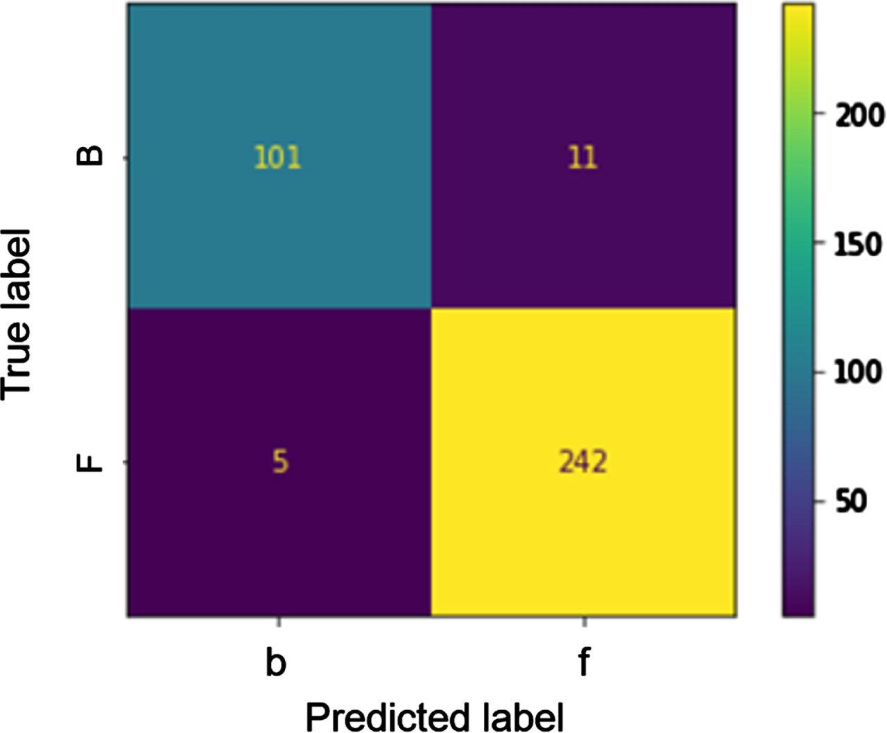
With respect to Fawcett (2006), in our case we do not deal with positive or negative, but with true (or predicted) locations in the front or in the back. With this respect, we refer to true front (fF, that is tags correctly located in the front by the classification method), true back (bB, that is tags correctly located in the back by the classification method), false front (fB) and false back (bF), with the true label being identified by capital letters (F and B), and predicted labels being identified by normal letters (f and b). With this respect, we define:
We note that the concept of accuracy and front accuracy are also used in standard confusion matrix, with the names of accuracy and recall (respectively). On the contrary, we introduce the concepts of Rear Accuracy and Percentage of False Front after brainstorming and discussion with store managers, software integrators, and academic colleagues. The former, in fact, allows us to estimate the percentage of tags that has been correctly located in the back and, consequently, the percentage of fB tags. Furthermore, the percentage of false front is used to identify, among all tags in the store, the percentage of those that have been located in the front, although they are not (i.e., fB tags).
Tables 4 7 report the results obtained by the different readers, reported in column, and by classification method, training data sets and power levels [mW ERP], reported in rows. These results are reported with average values of lines and columns, and they are detailed in average accuracy values of Equation 1 (reported in Table 4), average front accuracy values as in Equation 2 (and reported in Table 5), average rear accuracy values of Equation 3 (Table 6) and average percentages of false front, as detailed in Equation 4 (and whose results are reported in Table 7).
Accuracy per reader (column), by classification method, training data sets and power level in mW ERP (rows)
Accuracy per reader (column), by classification method, training data sets and power level in mW ERP (rows)
Front accuracy (same details of Table 4)
Rear accuracy (same details of Table 4)
Percentage of false front (same details of Table 4)
At first, we note that the overall accuracy of the different factors and levels tested in the two stores is of 0.90 (Table 4). This general value, however, can be achieved as an average of the two accuracies of reader A (0.94) and B (0.87). In particular, reader B with M2 classification method achieves a relatively low value of accuracy (0.81), with lower values of accuracy at higher power levels. Conversely, by means of reader A, higher values of accuracy can be achieved, especially by means of M2 classification method and at higher power levels (accuracy of 0.95–0.96). Also, due to the low performances of the M2 with reader B, this classification method results to perform worse than the M1 in terms of accuracy (with average values of 0.88 and 0.93, respectively).
Table 5 details the reasons behind the lower accuracy values of reader B with M2 its Front accuracy performances are definitely perfectible. The Front accuracy of the M2 with reader B is in fact below 0.70, with particularly low performances at higher reading power levels. Although this defect might be specific of the configuration of the classification method that we tested, we note that the application of M2 to reads from reader B has not been very effective in predicting the front label (f) for tags whose true label was in the front (F). On the contrary, the Front accuracy of reads from reader A is promising, with particularly high values of the M2 trained with front and back reads (0.96–97 Front accuracy).
The results of Table 6 add another interesting point of view on our results; although all methods and trainings perform relatively well in terms of Rear accuracy, reader B looks much more promising from this point of view, with Rear accuracy values as high as 0.99–1.00 (M2 trained with front reads only) that never drop below 0.94, regardless of the power level, training data set and classification method. Indeed, reader A also performs relatively well in terms of Rear accuracy, with an average value of 0.93, and better results with the use of front and back reads as training data sets and higher power levels.
These results are of course in line with the percentages of false front, which sees much better results produced by reader B, with an average percentage of false front of 0.01, and most data below 0.02, regardless of the power levels, training data sets and classification method. As it can be expected from what was stated so far, the reader A slightly underperformed in terms of percentage of false front, with values between 0.02 and 0.05 and no clear path that can lead to identify differences in performance based on the mentioned variables.
Lastly, we stress the fact that the two different stores do not produce significantly different data, in terms of all the output variables of Section 3.7, as it has been confirmed by a test on the analysis of variance (ANOVA) with p value equal to 0.05.
In this paper, the RFID SBS solution proposed by G. Esposito, and Romagnoli (2021) is investigated in real-life environments, i.e., in two different fashion retail stores located in Northern Italy (Bologna and Milan, respectively). The proposed solution relies on item-level RFID tags, and it particularly suits the needs of the fashion and apparel sector, providing flexibility and, possibly, economic savings, as it can classify tags belonging to different store areas without a physical shielding between the very same areas. In the present study, SBS has been tested with different factors and levels, that is (i) reader models, (ii) power levels, (iii) classification methods, and (iv) training data sets. Also, reference tags have been introduced in the present work, to support both the classification methods. The output variables upon which the factors and levels were compared are their accuracy (overall, front, and rear accuracy, as in Equation 1–3) and the percentage of false front.
Firstly, we note that the two stores were operating during testing activities, so our results have been collected in normal working conditions. In these circumstances, SBS proves to be a viable solution, although some more testing and fine tuning is still requested to identify its best working conditions in a robust way. Also, we note that the use of reference tags has proved to be quite inexpensive, and non-intrusive, with respect to store operations. The overall accuracy of all factors and level tested is of 0.90, with the reader A performing better than the reader B in terms of overall and front accuracy (both values of 0.94 with reader A, against 0.87 and 0.79 of reader B). Reader B, on the contrary, has proved to perform better in terms of rear accuracy, and percentage of false front (0.98 and 0.01, respectively, against the values of 0.93 and 0.03 of reader A). From these values, we can deduce the fact that, despite the different power levels, classification methods, and training data sets, reads from reader B are more likely to be classified in the back, to the detriment of both front and overall accuracy values. Reads from reader A, on the contrary, provide higher overall and front accuracy, at the price of higher percentages of false front. We note that false front is particularly undesired by store managers, as they relate to items that are indicated in the front (and therefore not considered for replenishment), while they are not, with potential generation of lost sales.
With respect to the classification method, no clear indications emerge from our study on the best performing one. M2, in fact, performs slightly better than M1 with reader A, but the contrary is true if we consider reads from reader B. In particular, the application of M2 to the reads from reader B has performed very bad in terms of front accuracy. Despite this mistake could be linked to the specific selection and tuning of the classification method that we used, we have not yet identified the possible cause behind these data, and therefore we call to action for more research on this point.
With respect to the training data, we note that, given the same reader model and classification method, when front and back reads data are used for training, the results are almost always better than the training with sole front data. This result suggests more research on the training of classification models with different data sets, regardless of the specific method used. Lastly, no clear indication can be drawn by the different power levels. Our results, in fact, are not importantly connected to the reading power levels, thus suggesting that both selective and massive inventory counts can by supported by SBS.
The limitations of the present study can be summarised as follows: first, we considered a given set of factors and levels, which could definitely be expanded and improved (e.g., different readers, power levels). Also, only a specific setting of each of the two classification methods M1 and M2 was tested. We used similar methods to those applied in prior research, but we urgently call for more research on this topic, so as to allow comparison with different methods and algorithms suggested by other colleagues. Another limitation is the fact that we could not consider tags disposition and density in the present study. As Neroni et al. (2022) recently proved, both tags disposition and density are impactful surrounding conditions for the performances of SBS. Unfortunately, we needed to adapt the design of our research to the real store conditions on the testing days, so it was not possible for us to produce too much disturbance to normal store operations. We are already working on some of these points for future research.