Sage Journals: Discover world-class research

Abstract

Osteoporosis is a disorder, that leads to fractures and fatal problems in bones. It is believed that more than 200 million individuals are affected globally. Furthermore, osteoporosis is caused by micro-architectural degeneration of bone tissues, which increases the risk of bone fragility and fractures. Moreover, the osteoporosis categorization is essential for the medical industry, which classifies the skeleton problems of individuals caused by ageing. This work presented the prediction of femur bone volume for osteoporosis classification. Moreover, the femur bone X-ray image is utilized for the classification. The preprocessing phase is employed to neglect the noise contained in input bone images through a non-local means filter. In the image segmentation process, the SegNet is utilized to isolate the specific portion. Moreover, the template search approach based on femoral geometric estimation is carried out and the feature extraction phase is essential for a significant feature extraction process. The proposed tuna jellyfish optimization based deep batch-normalized eLU AlexNet (DbneAlexNet) is utilized in the osteoporosis classification process. Furthermore, accuracy, Positive Predictive Value (PPV), Negative Predictive Value (NPV), True Positive Rate (TPR) and True Negative Rate (TNR) are the metrics to validate the model and the superior values 0.913, 0.906, 0.896, 0.923 and 0.932 are achieved.

Keywords

Femur bone osteoporosis classification jelly fish search optimization tuna swarm optimization deep batch-normalized eLU AlexNet

1. Introduction

The femur bone can be referred to as the thigh bone. Moreover, it is the lengthy, largest and heaviest bone. This bone’s length is nearly 26% of the height of the individual. The femur bone is separated into three sections, which include the upper extremity, the body, and the lower extremity. The upper section is made up of the neck, head and two trochanters. The body is a long and cylindrical structure, that is slightly curved. The lower extremities are larger than the upper extremities. It is slightly cuboid in shape, but its diagonal diameter is bigger than its anteroposterior [23]. Moreover, osteoporosis is a form of skeletal illness defined by a reduced mass of bones. It is restricted by the microstructure of bone cells, which increases the susceptibility and fragility to fractures. In 2019, there were 32 million people were affected in Europe. This growth is regulated by the lifestyle aspects such as food and physical movement. Thus, it can be expected that the pandemic will worsen the situation and significantly affect the person [11]. If osteoporosis is not identified in the early stage, then the bones are affected by osteoporotic fractures and it is more dangerous in the spine. Therefore, continuous research is necessary to develop the best diagnostic method that would allow the detection of osteoporosis at an early stage of development [27, 17].

Osteoporosis is commonly known as a chronic illness, in which the bones are weakened increasing the possibility of fractures. This condition is overlooked and relatively quiet because the consequences are only felt when the fracture has happened. This asymptomatic condition is a complicated health issue affecting women, in which approximately 80% of them are in the postmenopausal stage. If they are not treated or prevented properly, it may cause severe injuries. Normally, individuals have a certain quantity of minerals and calcium present in a specific region of the bone. If this quantity increases significantly, then the bones become more denser, tougher and less likely to break. Hence, the earlier prediction of osteoporosis minimized the risk of bone crack. A person suffering from osteoporosis is susceptible to fractures which cause serious damage to bones. In such cases, a very small amount of pressure is applied on the bone to perform their daily activities, which does not affect a healthy bone [24]. The common method for detecting osteoporosis is the calculation of Bone Mineral Density (BMD) [6] and BMD estimates the thickness of bones via X-rays. The BMD test is employed for estimating the T-score of the body. The T-score of a person’s bone density report is used to calculate the difference between his/her BMD to that of a healthy 30-year-old [24].

Osteoporosis condition has become more prevalent with the rise of the ageing population. It is a critical, multi-factorial health issue. This is a social as well as a health issue that must be treated in the earlier period. In recent years, the clinically relevant approaches for diagnosing osteoporosis have been split into two categories, they are invasive and non-invasive examination. Moreover, the invasive examination utilizes histomorphometry, whereas the non-invasive examination comprises biochemical testing, medical imaging, bone density assessment and so on. There are many imaging diagnostic methods for osteoporosis including dual-energy X-ray absorptiometry (DEXA) [6], quantitative computed tomography (QCT) [29], quantitative ultrasound (QUS) [28], magnetic Resonance check diagnosis (including diffusion-weighted imaging (DWI) [9], ultrashort echo (UTE), magnetic resonance imaging (MRI), high-resolution magnetic resonance imaging (HRMR), magnetic resonance spectroscopy (MRS) and so on [5]. In medical image processing, deep learning models including convolutional neural networks (CNN) have demonstrated considerable efficacy. Moreover, the Deep CNN (DCNN) is a deep learning method, that has been gaining a significant role in computer vision. The deep learning uses the image pixels and their relevant classes of medical images and consequent learning for feature description. Numerous early studies have also shown the promising results of DCNN used in a variety of medical imaging including radiology, pathology, dermatology, and ophthalmology [2].

1.1 Motivation

Bone X-ray images are widely regarded as the most effective approach for diagnosing osteoporosis and predicting the risk for fractures. For this, several methodologies were used, but it was still expensive and required a longer time for osteoporosis detection. Therefore, this research utilized a hybrid optimization-enabled deep learning technique for effectually identifying osteoporosis.

1.2 Main contribution

A prime objective is to model a reliable methodology for categorizing osteoporosis using X-ray images. Here, the Non-Local Means (NLM) filter is employed in the preprocessing, and then the noise from the image is neglected. Moreover, the SegNet is utilized for segmenting the bone image. Following, that, the template search approach is employed for estimating the femoral geometry. Afterwards, the Grey Level Co-occurrence Matrix (GLCM), medical feature, Local Vector Pattern (LVP) feature, Pyramid histogram of orientation gradient (PHoG) features and CNN features are extracted. Finally, osteoporosis classification is done by DbneAlexNet, where its hyperparameters training is done via the proposed tuna jellyfish optimization.

The crucial contribution is elucidated as follows: tuna jellyfish optimization based DbneAlexNet for osteoporosis classification: A novel model is developed for femur bone volumetric estimation based osteoporosis classification, utilizing the tuna jellyfish optimization based DbneAlexNet. Here, the hyperparameters present in the DbneAlexNet are trained using tuna jellyfish optimization. Furthermore, the tuna jellyfish optimization is obtained by a merging of tuna swarm optimization with jellyfish search optimizer.

1.3 Structural organization

This paper is labelled in the following way: The traditional methodologies in osteoporosis classification are explained in Section 2 and the proposed osteoporosis prediction is defined in Section 3. The experimental result of the proposed technique is explained in Section 4. Furthermore, the conclusion is illustrated in Section 5.

2. Literature review

Shankar et al. [16] developed the Gradient Harmony Search based Deep Belief Network for osteoporosis detection. Here, preprocessing, segmentation, geometric evaluation, feature extraction and osteoporosis categorization are the five procedures used in osteoporosis classification. Moreover, the gradient descent required less computation time and less storage. Nonetheless, it failed to consider the advanced segmentation techniques for attaining even more precise performance. Nazia Fathima et al. [21] devised the modified U-net for BMD estimation. Here, the linear regression model was designed to evaluate the BMD. It obtained higher classification accuracy for DEXA and X-ray images. Still, it did not produce a reliable outcome in real-time applications. Liu et al. [5] developed the deep U-Net model for osteoporosis diagnosis. In this, the input image pattern on each layer was identical. This approach produced a precise categorization result and effectively minimized the influence of image distortion in BMD measurement. Still, the processing time was high. Suzuki et al. [22] devised a mandibular cortical index (MCI) and mandibular cortical widths (MCW) based osteoporosis classification. During orthopedics treatment, the patients were subjected to BMD and panoramic radiography tests. This approach required a little storage space. However, it failed to assess the prevalence of cortical bone porosity throughout the body. Prakash et al. [24] developed the 4x-expert system for osteoporosis segmentation and detection, which employed a multi-model machine learning algorithm to improve prediction accuracy. This method provided segmentation outcomes via the quick processes and it offered flexible features. Nonetheless, it offered poor reliability in real-time usage. Shaker [1] developed the Recurrent Neural Network (RNN) based osteoporosis detection method. The osteoporotic fractures were predicted using spine images. This approach was suitable for larger datasets and it failed to utilize the DEXA images for osteoporosis prediction. Shahzad et al. [14] developed the osteoporosis classification model using CNN. It was more efficient in terms of extracting more features. This approach effectively identified the bone volume and predicted osteoporosis effectively. However, the sensitivity level was too low. Su et al. [18] developed the fusion of CNN and handcrafted features (CNN $+$ handcrafted) for diagnosing osteoporosis. The high dimensionality of the features was reduced using a minimum-redundancy maximum-relevance approach. Furthermore, it attained the finest features and improved its performance. Nonetheless, it needed more iteration levels to provide the outcome.

2.1 Major challenges

Some of the challenges faced by the classical techniques for osteoporosis classification are listed below:

The method [22] did not use deep learning based Artificial Intelligence approach. Since the raising quantity of training samples did not enhance the diagnostic accuracy. Furthermore, it failed to include the creation of software for performing the Mandibular cortical index (MCI) categorization on the cortex of the limb’s bones. The RNN accurately predict osteoporotic fractures based on spine scans. However, the dataset employed in this method was very small, and it failed to represent the complete range of real-time feature space [1]. The CNN model [14] provided clear visualization, since, the visualizations of pre-trained models were more difficult to classify the femur bones. Moreover, it produced fewer notable outcomes. The CNN $+$ handcrafted features [18] have the greatest accuracy and specificity. However, it did not incorporate the advanced CNN features and did not provide enhanced handcrafted features to improve diagnostic accuracy. The deep learning methods required a vast amount of data to attain accurate classification. Due to the complexity of the data models, the training process was quite expensive. Furthermore, the deep learning model necessitates the use of costly GPUs and hundreds of workstations.

3. Proposed tuna jellyfish optimization based DbneAlexNet for osteoporosis classification

The crucial role of this research is to build the osteoporosis classification model using the proposed tuna jellyfish optimization. Initially, the input femur bone image is subjected to the pre-processing module, where the noises present in the image are removed using an NLM filter [19]. After that, the femur boundary segmentation is carried out using the SegNet [25]. After segmentation, the femoral geometry measurement is done using the template search method [16]. Thereafter, the feature extraction is carried out to extract the GLCM texture features [3, 15], medical level features, LVP feature [10], PHoG feature [26], and CNN features [18]. Here, the GLCM features include the Angular Second Moment (ASM), correlation, contrast, Inverse Difference Moment (IDM), entropy and homogeneity. On the other hand, medical-level features [16] include Hip Axis Length (HAL), Femoral Neck Axis Length (FNAL), Femoral Head Diameter (FHD), Femoral Neck Width (FNW), Neck Shaft Angle (NSA), and shaft width. Following this, the osteoporosis classification is performed by the DbneAlexNet [4], where the parameters of DbneAlexNet are trained by the proposed tuna jellyfish optimization algorithm. Finally, the osteoporosis classification is obtained. Figure 1 represents a block diagram of tuna jellyfish optimization based DbneAlexNet for osteoporosis classification.

Figure 1.

Block diagram of tuna jellyfish optimization based DbneAlexNet for osteoporosis classification.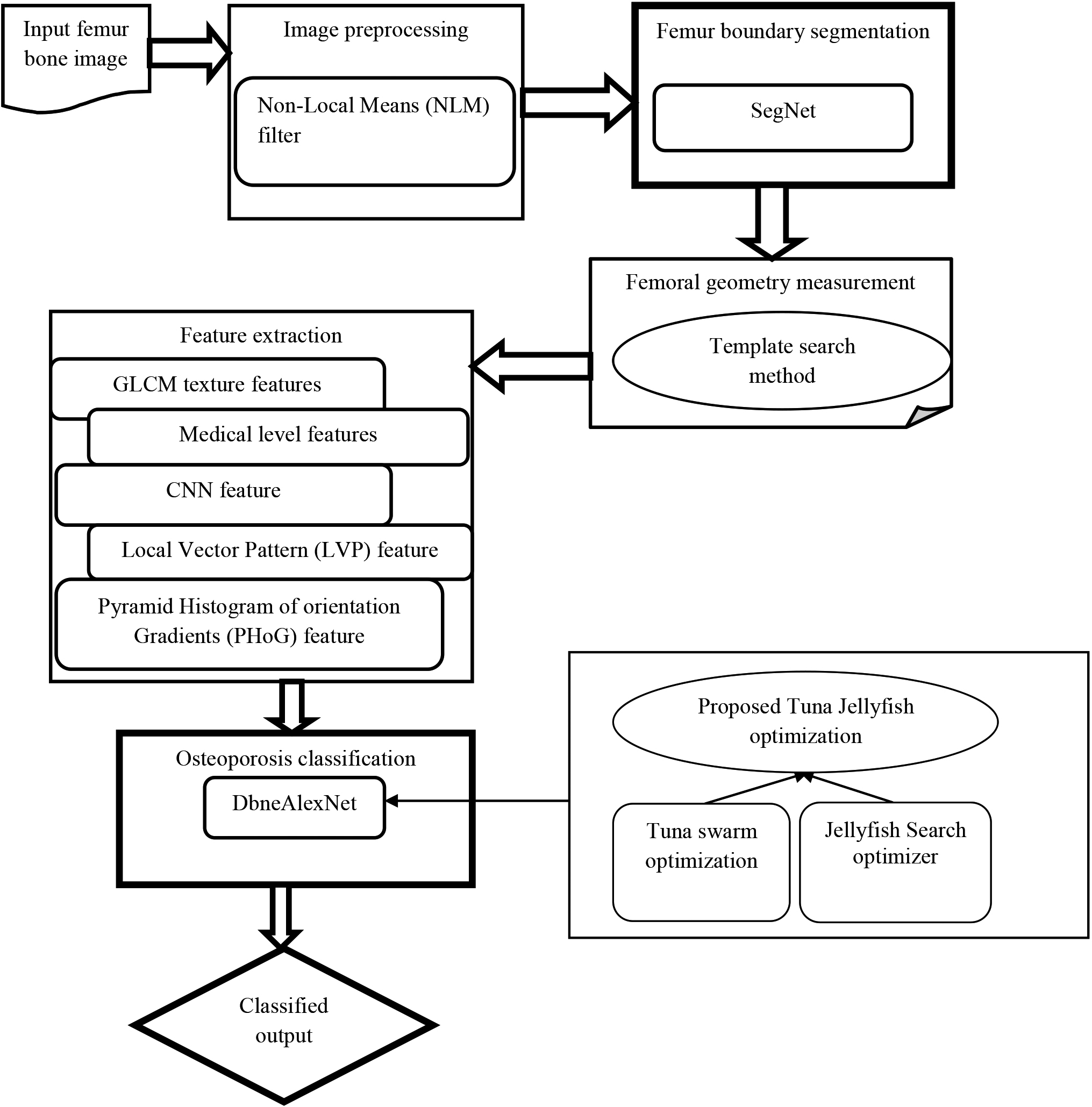

3.1 Image acquisition

Input femur bone image is gathered through a dataset $B$ , where the entire count of this image is represented as $y$ . The dataset is represented as follows,

$\displaystyle B=\{{B_{1},B_{2},\ldots,B_{n},\ldots,B_{y}}\}$ (1)

where the whole counting of the image is denoted as $y$ and $n^{\text{th}}$ image is denoted by $B_{n}$ .

3.2 Image preprocessing using non-local means filter

Preprocessing is the initial step, where noise is reduced. Here, the noise present in the images is filtered out using the NLM [19] filter. The input image $B_{n}$ is applied for the preprocessing stage, where it contains the original image $(s)$ and a noise $(t)$ . It is denoted as $B_{n}=s+t$ in which the NLM evaluate the noiseless image $\widehat{s}_{\textit{NLM}}(v)$ of pixel $v$ is given as,

$\displaystyle\widehat{s}_{\textit{NLM}}(v)=\sum\limits_{w\in\Omega B_{n}}% \varpi({v,w})B_{n}$ (2)

where $\Omega B_{n}$ specifies the entire image. The weight $\varpi({v,w})$ amongst the original pixel $B_{n}$ and target pixel $s(v)$ is represented as,

$\displaystyle\varpi({v,w})=\frac{1}{E_{v}}\exp\left\{{-\frac{\|{B_{n}({\sigma_% {v}})-B_{n}({\sigma_{w}})}\|_{2,\Im}^{2}}{\ell}}\right\}$ (3)

where $E_{v}$ represents the normalizing factor, in which $\sum\varpi({v,w})=1$ , $B_{n}({\sigma_{v}})$ specifies the neighborhood, $\sigma_{w}$ indicates the centred around the pixel $v$ of the noisy image, $||.||_{2,\Im}^{2}$ denotes the Euclidean norm of Gaussian kernel with standard deviation $\Im$ , and the parameter $\ell$ alters the decay of weight. Moreover, the outcome of NLM is denoted as $B_{o}$ .

3.3 Femur boundary segmentation

The pre-processed image $B_{o}$ is given to the femur boundary segmentation phase, where SegNet is used to identify the femur areas. Hence, the femur region is segmented for further processing. The structure of SegNet is presented as follows.

Figure 2.

Architecture of SegNet.

3.3.1 Architecture of SegNet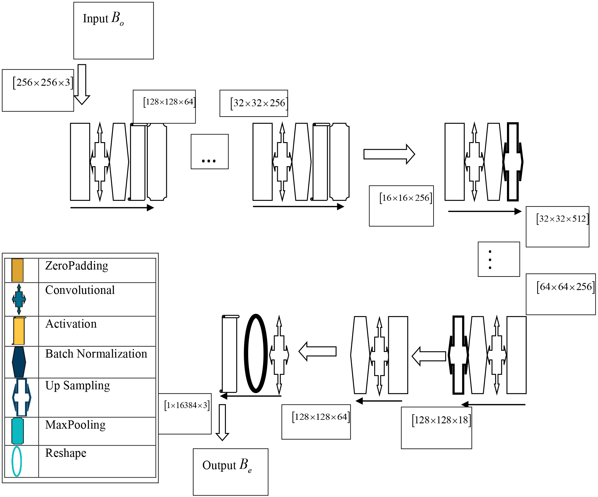

SegNet [25] is the encoder network, where the corresponding decoder network follows the final layer for pixel-based classification. The structural depiction of SegNet is given in Fig. 2. The encoder has 13 convolutional layers, and training is conducted with weights. Furthermore, the fully connected (FC) layers are removed to get a higher-resolution feature map. The training of the decoder filter without the feature maps is convoluted by the SegNet, which employs the max-pooling function and directs the upsample. Furthermore, SegNethass is the decoder that increases the resolution of the input feature maps. Additionally, a decoder utilized a pooling index to assess a linked max-pooling of the encoder and non-linear upsampling. As a result, the dense feature map is created by conserving the upsample maps and convolving them with trainable filters. The segmentation output is represented as $B_{e}$ .

3.4 Femur geometry measurement

The template search approach [16] computes the important locations in the femur segment while measuring the femur geometry. The femoral boundary measurement is utilized for computing the numerous medical-level features. Moreover, the effective prediction of femur geometry is needed to find the fracture risks and bone strength. The methods required to measure the geometry of the femurs are shown in Fig. 3. Here, the segmented femur image $B_{e}$ is applied as the input of femur geometry measurement.

Step 1:
Application of Circular Hough transform: It is used to determine the circle’s center by detecting a circular patch of the femur segment. The ideal center is denoted by $P$ , which is the center point.
Step 2:
Find the points $S$ and $X$ : The horizontal line is marked across an ideal center and then the angle $({\angle 35})$ is pointed on the horizontal line. Moreover, the line is marked to the ideal center to reach a femoral boundary $S$ and $X$ .
Step 3:
Mark the point $P$ and point $R$ : The distance amongst the points $S$ and $X$ is calculated by dividing this distance by 8. Point $S$ moved outward to meet $R$ , that is a distance from $S$ .
Step 4:
Create a perpendicular bisector to $P$ : A vertical bisector is constructed for a line $R X$ as its center point $P$ , which intersects at locations $P$ and $T$ . Furthermore, a parallel line $Y U$ is marked and the horizontal line $Z T$ is drawn on a point $Y$ that intersects three locations at the femoral region.
Step 5:
Detecta point $Q$ : Points $V$ and $W$ are connected to create a femoral shaft, in which a line from a middle point of $V W$ meet $R X$ on point $Q$ . Moreover, these points are calculated in an optimum way by the template search approach, which automatically calculates the important points from the femoral limits and computes the medical level feature. The outcome of template search based geometric measurement is represented by $B_{\hbar}$ .

Figure 3.
Femur bone structure.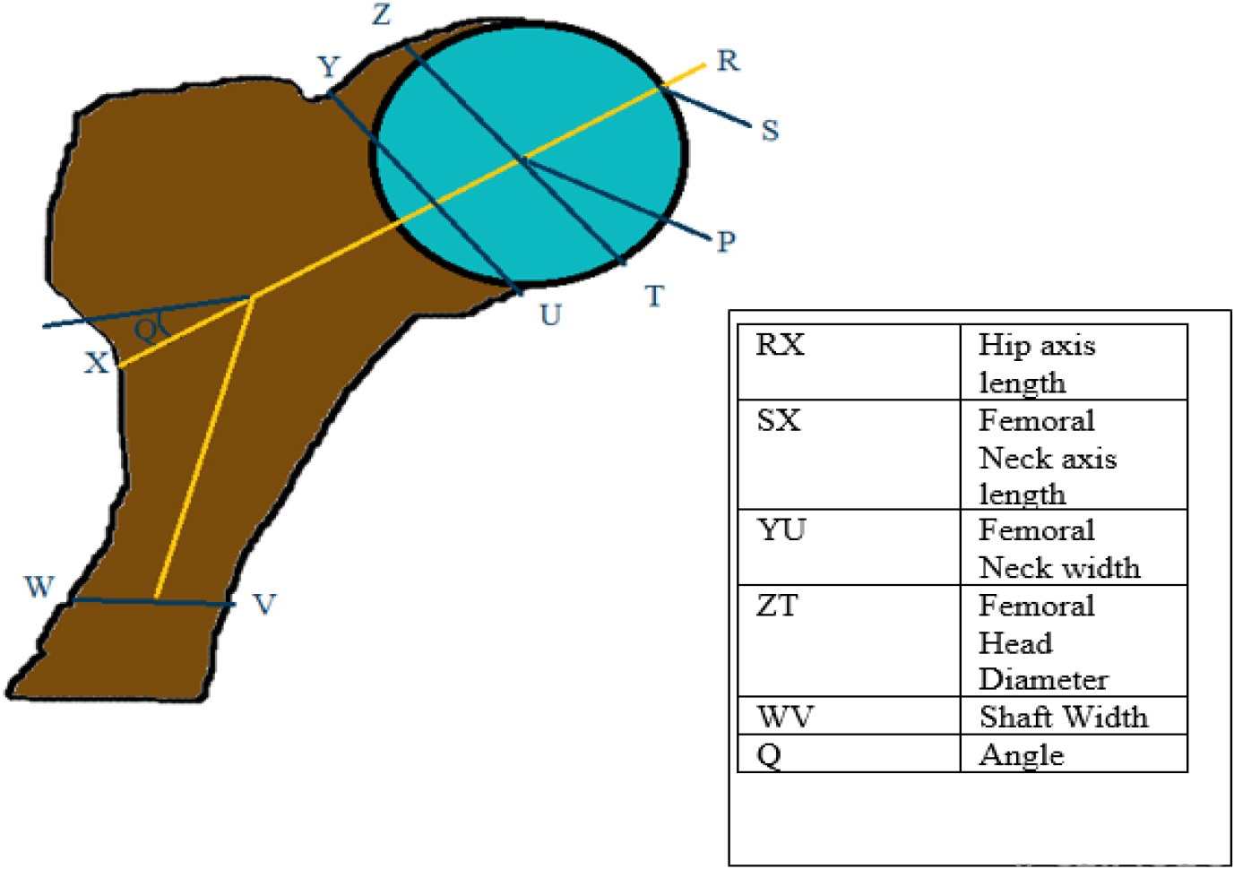

3.5 Feature extraction

The image after femur geometry measurement $B_{\hbar}$ is applied to feature extraction. Here, the important features have been extracted to provide the prediction process effectively. Moreover, the GLCM, medical features, LVP, CNN and PHoG features are extracted.

3.5.1 Grey level co-occurrence matrix (GLCM) texture features

To achieve spatial dependency amongst the image pixels, the GLCM features [3, 15] are used. The GLCM is a kind of matrix having the counts of columns and rows are equivalent to grey levels. The pixel distance $({\Delta_{\beta},\Delta_{\gamma}})$ is applied to separate the matrix elements $F({I,J|\Delta_{\beta},\Delta_{\gamma}})$ using the frequency level and the statistical measurements. Still, it is primarily applied to grey-level image matrices for getting important features like ASM, contrast, correlation, entropy, and IDM. Here, the $B_{\hbar}$ is applied as the input of the feature extraction technique.

Angular Second Moment ASM [3] is defined as the addition of squares of the image’s grey levels. It is also referred to as energy. Whenever the intensity levels are asymmetrical, the ASM value is increased. Moreover, ASM is specified as $\mathbb{N}_{1}$ .

$\displaystyle\mathbb{N}_{1}=\sum\limits_{I}{\sum\limits_{J}{\{{B_{e}({I,J})}\}% ^{2}}}$ (4)

where $B_{e}({I,J})$ implies the image with a pixel element $({I,J})$ .

Contrast [3] measures the brightness of an image. If the image pixels have similar intensity, then the contrast value is low. Moreover, contrast is denoted as $\mathbb{N}_{2}$ .

$\displaystyle\mathbb{N}_{2}=\sum\limits_{i=0}^{K-1}i^{2}\left\{{\sum\limits_{I% =1}^{K}{\sum\limits_{J=1}^{K}{B_{e}({I,J})}}}\right\}$ (5)

where $K$ signifies a grey level of the image.

Correlation [3] is described as an index of grey value dependence and is expressed as a portion of the comparability of the pixel to its neighboring measurement. Therefore, the correlation expression is denoted as $\mathbb{N}_{3}$ .

$\displaystyle\mathbb{N}_{3}=\frac{\mathbb{N}_{1}=\sum\limits_{I}{\sum\limits_{% J}{({IJ})B_{e}({I,J})-\vartheta_{\varsigma}\vartheta_{\wp}}}}{\lambda_{% \varsigma}\lambda_{\wp}}$ (6)

where $\lambda_{\varsigma},\lambda_{\wp},\vartheta_{\varsigma},\vartheta_{\wp}$ represents the standard deviation and mean of the image $B_{e}$ .

Entropy [3] is utilized for predicting the heterogeneity of the images. It is a statistical aspect for specifying the texture data of an image. It is given by $\mathbb{N}_{4}$ .

$\displaystyle\mathbb{N}_{4}=-\sum\limits_{I}{\sum\limits_{I}{B_{e}({I,J})}}% \log({B_{e}({I,J})})$ (7)

Inverse Difference Moment (IDM) [3] specifics the smoothness of the image. If the grey value of the pixels matches, the IDM value is high. Furthermore, the IDM is written as $\mathbb{N}_{5}$ .

$\displaystyle\mathbb{N}_{5}=\sum\limits_{I}\sum\limits_{j}\frac{1}{1+({I-J})^{% 2}}B_{e}(I,J)$ (8)

Homogeneity [15] offers the degree of measurement that determines the proximity of the origin. Moreover, the homogeneity is denoted as $\mathbb{N}_{6}$ .

$\displaystyle\mathbb{N}_{6}=\sum\limits_{I,J}{\frac{C({I,J})}{1+|{I-J}|}}$ (9)

To attain a smooth output, it is required to identify all points $C({I,J})$ of the image.

3.5.2 Medical level features

The medical level features [16] are essential for effective classification, and they enhance the classification accuracy. Moreover, Hip Axis Length (HAL), Femoral Neck Axis Length (FNAL), Femoral Head Diameter (FHD), Femoral Neck Width (FNW), Neck Shaft Angle (NSA), and shaft width are medical features, which are extracted by a geometric point and that are predicted by the automatic template search technique. Moreover, the medical feature is attained from Fig. 3.

Hip Axis Length (HAL) is a measurement of the distance between the bigger trochanter as well as its inner pelvic brim. Here the points $R$ and $X$ specifies the bigger trochanter and the inner pelvic brim, which are used to calculate hip axis length. In longer HAL, there is more probability of fractures. Here, $\mathbb{N}_{7}$ represents the HAL feature.

Femoral Neck Axis Length (FNAL) is the distance between the bigger trochanter $(S)$ and the vertex of the femoral head $X$ . Figure 3 depicts the locations A and G. Moreover, the FNAL is necessary while the femurs are separated from the conjunctive tissues and there is no attachment to the pelvic region. Here, the FNAL feature is symbolized as $\mathbb{N}_{8}$ .

Femoral Head Diameter (FHD) is the distance amongst the geometric point $Z$ and $T$ , while the greatest value of femoral head diameter and it is necessary to measure the bone strength. Moreover, $\mathbb{N}_{9}$ indicates the FHD feature.

Femoral Neck Width (FNW) is the shorter distance, which is vertical to a neck axis with the femoral neck. Furthermore, FNW is the distance between the points $W$ and $X$ . If the FNW is less, there is a greater risk of bone injury. However, FNW is related to age, body size, and other aspects. Here, $\mathbb{N}_{10}$ indicates the FNW feature.

Neck Shaft Angle (NSA) $({\angle Q})$ is termed as an angle created among the femoral neck and shaft axis. The average NSA in adults is reported about 120⁰ to 135⁰, and it fluctuates by the level of physical activity. Furthermore, the NSA feature is indicated as $\mathbb{N}_{11}$ .

Shaft width implies a width of the femur below the trochanter minor, and a line $V W$ illustrates the shaft width. Here, $\mathbb{N}_{12}$ represents the shaft width.

3.5.3 Local Vector Pattern (LVP) feature

Local Vector Pattern (LVP) [10] represents a one-dimensional texture pattern and generates a structure-related image. It determines the referenced and pixel values at various distances and angles. Moreover, a vector direction $\Re_{\varphi,\theta}(\mathbb{Z}_{\phi})$ in a reference pixel $\mathbb{Z}_{\phi}$ at the local sub-region $\mathbb{C}$ is represented as,

$\displaystyle\Re_{\varphi,\theta}(\mathbb{Z}_{\phi})=(\mathbb{C}(\mathbb{Z}_{% \varphi,\theta})-\mathbb{C}(\mathbb{Z}_{\phi}))$ (10)

where $\varphi$ specifies a direction of adjacent as well as referenced pixel, distance amongst the adjacent and adjutant pixels are denoted as $\theta$ . In referred pixels, LVP utilizes four pairwise vector directions. With the aid of the transform ratio, the weight vector for the dynamic linear function is fixed via the 8-bit binary sequence. Additionally, $\mathbb{N}_{13}$ implies the LVP features.

3.5.4 Pyramid histogram of orientation gradients (PHOG) feature

A histogram of orientation gradients (HoG) over each image sub-region at each resolution level constitutes the pyramid histogram of orientation gradients (PHOG) descriptor [26]. To do this, every image is composed of a series of increasingly finer spatial grids through the doubling of divisions in every direction (similar to a quadtree). The PHOG descriptor is an HoG, that covers a sub-region on every image resolution. Moreover, the PHOG features are obtained in the following way.

Step 1:
Initially an edge curve of an image is extracted for the following steps.
Step 2:
The cells are isolated from the images by multiple pyramidic levels.
Step 3:
In each stage of pyramid resolution, the HOG of every grid was calculated. Moreover, a local shape is denoted via an edge orientation histogram. Moreover, step 1 involved the location of the edge contour of an original image and calculating an orientation gradient.
Step 4:
All HOG vectors of a pyramid resolution are combined to generate PHOG-featured images. By combining all HOG vectors, spatial data is captured. Several pyramid levels are considered and each HOG is connected to unity. Furthermore, the PHOG features are indicated as $\mathbb{N}_{14}$ .

3.5.5 CNN features

The CNN [18] is made up of convolutional layers, pooling (POOL) layers, and an FC layer, which is deliberated in Fig. 4. Normally, input $B_{\hbar}$ is passed to the convolutional layer. A significant layer in CNN is the convolutional layer, which has several subsequent layers. Here, an outcome of the prior layer is given to the present layers, which is utilized to get an outcome of the FC layer. To facilitate the underlying processing, convolutional networks are integrated into global and local pooling. The pooling layer provides a fixed function, and it is the subsampling layer to decreases the solution of the feature map and boosts up the uniformity of the input image. The CNN feature is specified as $\mathbb{N}_{15}$ .

Figure 4.

CNN feature.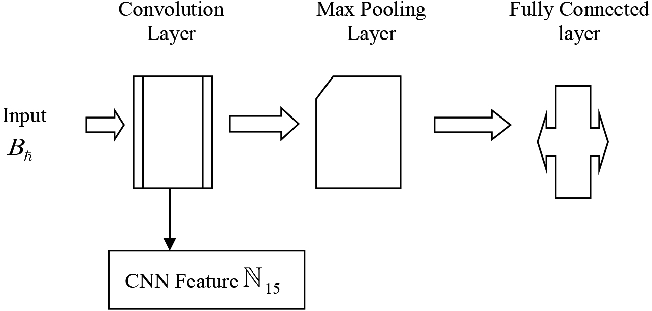

Here, a feature vector $\mathbb{N}$ implies an outcome of feature extraction, which is expressed as follows,

$\displaystyle\mathbb{N}=\{{\mathbb{N}_{1},\mathbb{N}_{2},\ldots,\mathbb{N}_{15% }}\}$ (11)

3.6 Osteoporosis classification

In the osteoporosis classification stage, the DbneAlexNet is employed. Here, the tuna jellyfish optimization algorithm is utilized for the training process of DbneAlexNet. The DbneAlexNet has faster learning as well as convergence speed. Here, a feature vector $\mathbb{N}$ is utilized as an input to the classification phase. Furthermore, the model description and training process of tuna jellyfish optimization enabled DbneAlexNet are illustrated as follows.

3.6.1 Architecture of DbneAlexNet

The DbneAlexNet [4] contains the convolutional layer, which is followed by batch normalization, Max pooling, flattening, dense layer and dropout layers. Figure 5 illustratesa structure of DbneAlexNet. In this, a feature vector $\mathbb{N}$ is given as an input to DbneAlexNet. The exponential linear unit (Elu) activation layer is utilized instead of the rectified linear unit (ReLU). Furthermore, the internal covariate shift concerns are resolved by batch normalization. It is done by altering a count of variables in the prior one. Dropout is another layer of DbneAlexNet. In training, a dropout mechanism is used to ignore a randomly selected neuron. Furthermore, $\mathbb{N}_{\xi}^{\textit{Dbne}}$ implies the outcome of DbneAlexNet.

Figure 5.

Structure of DbneAlexNet.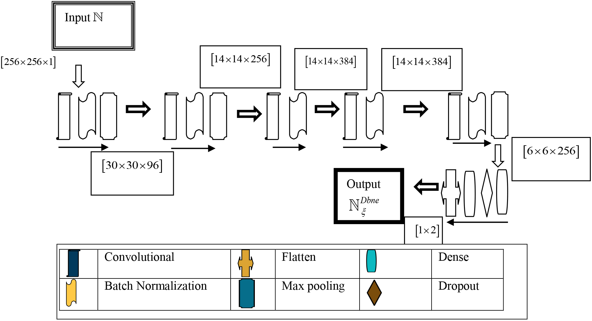

3.6.2 Training of DbneAlexNet by proposed tuna jellyfish optimization

The parameters of DbneAlexNet are tuned using the proposed tuna jellyfish optimization. Moreover, the merging of tuna swarm optimization [13] and jellyfish search optimizer [7] formed the tuna jellyfish optimization. Here, tuna swarm optimization depends on the Tuna fish’s cooperative hunting behaviour. The Tuna is scientifically known as Thunnini, which is a carnivore sea fish. There are different kinds of tuna categories, and their sizes are varied. Tuna are the top aquatic predators that eat a wide range of surface and midwater live species. In addition, the tunas have persistent swimming behavior with a distinct effective swimming style. As a result, tuna will employ a “group travel approach for prediction”. They hunt and attack the prey using their intellectual abilities. Moreover, spiral and parabolic foraging are the two powerful and clever foraging strategies of tuna swarms. Moreover, it has higher robustness and scalability to provide the finest solution. Furthermore, the jellyfish search optimizer is combined with tuna swarm optimization to diminish the computational complexity. Jellyfish search optimizer [7] is based on the behaviors of jellyfish, which exist in a variety of depths and environmental conditions in the deep sea. They appear as bell-shaped and utilized their limbs to harm an object. Moreover, they do not harm people, though anybody who swims up to them or comes into contact with them is affected. Furthermore, jellyfish bloom is produced by the ocean circulation and specific attitudes of all jellyfish within the swarm. The movement is varied with respect to the food location. The optimal position of jellyfish is estimated by comparing the quantity of available food. It was utilized for resolving the structural optimization issues. Furthermore, these two algorithms are merged to attain the rate of convergence. The tuna jellyfish optimization are modelled in the following section:

Step 1: Population initialization

The initial population in tuna jellyfish optimization is generated randomly, which is given by,

$\displaystyle H_{a}^{\textit{Int}}=\textit{rand}.({b^{u}-b^{l}})+b^{l},a=1,2,\ldots M$ (12)

where $H_{a}^{\textit{Int}}$ represents the $a^{\text{th}}$ initial individual, $b^{u}$ and $b^{l}$ specifies an upper and lower boundary, $M$ implies the count of tuna and rand indicates a random vector, where it is regularly distributed in [0-1].

Step 2: Fitness Computation

Fitness is regarded as an important criterion for finding the finest solution. Moreover, the fitness function depends on the Mean Square Error (MSE) of the solution. Therefore, a solution provided with a minor MSE is considered as an optimum solution. The fitness is expressed as,

$\displaystyle\textit{Fitness}=\frac{1}{y}\,\sum\limits_{\xi=1}^{y}{[{\mathbb{N% }_{\xi}^{\ast}-\mathbb{N}_{\xi}^{\textit{Dbne}}}]^{2}}$ (13)

where the entire count of the images is specified by $y$ , $\mathbb{N}_{\xi}^{\ast}$ specifies the targeted outcome and $\mathbb{N}_{\xi}^{\textit{Dbne}}$ specifies the DbneAlexNet’s outcome.

Step 3: Spiral Foraging

Spiral foraging is the first strategy in tuna jellyfish optimization. At this point, the group of tuna fish chases the prey in a closely tight spiral shape. The majority of the fish do not have the awareness of selecting the direction, because a small group of these fish moves vigorously in one direction, whereas the neighboring fishes will change their direction. It generates a larger group with similar persistence for starting the hunting process. The mathematical model for the spiral foraging method is given by,

$\displaystyle H_{a}^{d+1}=\left\{{\begin{array}[]{ll}\rho_{1}.({H_{\textit{% best}}^{d}+\eta.|{H_{\textit{best}}^{d}-H_{a}^{d}}|})+\rho_{2}.H_{a}^{d},&a=1% \\ \rho_{1}.({H_{\textit{best}}^{d}+\eta.|{H_{\textit{best}}^{d}-H_{a}^{d}}|})+% \rho_{2}.H_{a-1}^{d},&a=2,3,\ldots,M\\ \end{array}}\right.$ (14) $\displaystyle\rho_{1}=g+({1-g}).\frac{d}{d_{\max}}$ (15) $\displaystyle\rho_{2}=({1-g})-({1-g}).\frac{d}{d_{\max}}$ (16) $\displaystyle\eta=e^{hc}.\cos({2\pi h})$ (17) $\displaystyle c=e^{3\cos({({(d_{\max}+1_{d})-1})\pi})}$ (18)

where $H_{a}^{d+1}$ denotes the $a^{\text{th}}$ individual of $d+1$ iteration, $H_{a}^{d+1}$ specifies $a^{\text{th}}$ individual on $d^{\text{th}}$ iteration, $H_{\textit{best}}^{d}$ represents the best individual on current location, $\rho_{1}$ and $\rho_{2}$ denotes weight coefficients for controlling the tendency of an individual moved to the optimal as well as previous individual, the constant $g$ is employed to find the optimal and previous individuals initial stage, $d$ represents the counting of present iteration, the maximum iterations is specified as $d_{\max}$ and $h$ depicts a random number, which lies in 0 and 1 range.

The tuna possesses strong exploitation capability in the search space for food. Moreover, it generates a random location on a search space and it is a reference point during the spiral searching phases. This allows every user to investigate a larger space and provides the tuna swarm optimization with worldwide exploration capability. The expression of updated search space is denoted as follows,

where $H_{\textit{rand}}^{d}$ implies the randomly produced reference point on a search space and $M$ specifies the size of the population. These algorithms typically create global exploration during an early stage. The mathematical form of the spiral foraging mechanism is given by,

$\displaystyle H_{a}^{d+1}=\left\{{\begin{array}[]{ll}\rho_{1}.({H_{\textit{% rand}}^{d}+\eta.|{H_{\textit{rand}}^{d}-H_{a}^{d}}|})+\rho_{2}.H_{a}^{d},&a=1,% \\ \rho_{1}.({H_{\textit{rand}}^{d}+\eta.|{H_{\textit{rand}}^{d}-H_{a}^{d}}|})+% \rho_{2}.H_{a-1}^{d},&a=2,3,\ldots,M,\quad\text{if }\textit{rand}<\frac{d}{d_{% \max}},\\ \rho_{1}.({H_{\textit{best}}^{d}+\eta.|{H_{\textit{best}}^{d}-H_{a}^{d}}|})+% \rho_{2}.H_{a}^{d},&a=1,\\ \rho_{1}.({H_{\textit{best}}^{d}+\eta.|{H_{\textit{best}}^{d}-H_{a}^{d}}|})+% \rho_{2}.H_{a-1}^{d},&a=2,3,\ldots,M,\quad\text{if }\textit{rand}\geqslant% \frac{d}{d_{\max}},\\ \end{array}}\right.$ (20)

Step 4: Parabolic Foraging: Parabolic foraging is the second strategy of tuna jellyfish optimization. Here, every tuna follows the previous one and constructs a parabolic curve that covers the prey. Furthermore, tuna search the food by looking around them. These two procedures are carried out concurrently. This specific model is expressed as follows,

$\displaystyle H_{a}^{d+1}=\left\{{\begin{array}[]{ll}H_{\textit{best}}^{d}+% \textit{rand}.({H_{\textit{best}}^{d}-H_{a}^{d}})+L.k^{2}.({H_{\textit{best}}^% {d}-H_{a}^{d}}),&\text{if }\textit{rand}<0.5,\\ L.k^{2}.H_{a}^{d}&\text{if }\textit{rand}\geqslant 0.5,\\ \end{array}}\right.$ (21)

where $L$ depicts a random value lie in ( $-$ 1 to1) and $k$ is given by,

$\displaystyle k=\left({1-\frac{d}{d_{\max}}}\right)^{\left({\raise 3.01pt\hbox% {$d$}\!\mathord{/{\vphantom{d{d_{\max}}}}.\kern-1.2pt}\!\lower 3.01pt\hbox{${d% _{\max}}$}}\right)}$ (22)

Consider $\textit{rand}<0.5$ , Eq. (22) is written as,

$\displaystyle H_{a}^{d+1}=H_{\textit{best}}^{d}+\textit{rand}.({H_{\textit{% best}}^{d}-H_{a}^{d}})+L.k^{2}.({H_{\textit{best}}^{d}-H_{a}^{d}})$ (23) $\displaystyle H_{a}^{d+1}=H_{\textit{best}}^{d}+\textit{rand}.H_{\textit{best}% }^{d}-\textit{rand}.H_{a}^{d}+L.k^{2}.H_{\textit{best}}^{d}-L.k^{2}.H_{a}^{d}$ (24) $\displaystyle H_{a}^{d+1}=H_{\textit{best}}^{d}({1+\textit{rand}+L.k^{2}})-H_{% a}^{d}({\textit{rand}+L.k^{2}})$ (25)

To improve the convergence speed, the jellyfish search optimizer [7] is merged in this phase, and the updated equation of tuna jellyfish optimization is expressed as follows,

$\displaystyle H_{a}^{d+1}=H_{a}^{d}+\alpha\times\textit{rand}({0,1})\times({B^% {u}-B^{l}})$ (26)

where upper and lower bounds are stated as $B^{u}$ and $B^{l}$ . The motion coefficient is represented as $\alpha$ . Moreover, $\alpha=0.1$ is considered for sensitivity assessment.

$\displaystyle H_{a}^{d}=H_{a}^{d+1}-\alpha\times\textit{rand}({0,1})\times({B^% {u}-B^{l}})$ (27)

Substitute Eq. (27) in Eq. (25),

$\displaystyle H_{a}^{d+1}=H_{\textit{best}}^{d}({1+\textit{rand}+L.k^{2}})-({H% _{a}^{d+1}-\alpha\times\textit{rand}({0,1})\times({B^{u}-B^{l}})({\textit{rand% }+L.k^{2}})})$ (28) $\displaystyle H_{a}^{d+1}+H_{a}^{d+1}({\textit{rand}+L.k^{2}})=H_{\textit{best% }}^{d}({1+\textit{rand}+L.k^{2}})+\alpha\times\textit{rand}({0,1})\times({B^{u% }-B^{l}})$ (29) $\displaystyle\quad({\textit{rand}+L.k^{2}})$ $\displaystyle H_{a}^{d+1}[{1+({\textit{rand}+L.k^{2}})}]=H_{\textit{best}}^{d}% ({1+\textit{rand}+L.k^{2}})+\alpha\times\textit{rand}({0,1})\times({B^{u}-B^{l% }})$ (30) $\displaystyle\quad({\textit{rand}+L.k^{2}})$ $\displaystyle H_{a}^{d+1}=\frac{1}{1+\textit{rand}+L.k^{2}}[H_{\textit{best}}^% {d}({1+\textit{rand}+L.k^{2}})+\alpha\times\textit{rand}({0,1})\times({B^{u}-B% ^{l}})$ (31) $\displaystyle\quad({\textit{rand}+L.k^{2}})]$

Equation (3.6.2) indicates the updated solution of tuna jellyfish optimization. For every iteration, all individuals randomly find one of the above-mentioned two foraging strategies and regenerate the location based on the probability $\delta$ .

Step 5: Re-estimation of Fitness

The overall fitness of an upgraded solution is found, where a solution that has minimal MSE is taken as an ideal solution.

Step 6: Termination

Continued the iteration till the ideal solution is reached. Moreover, Algorithm 1 represents the pseudocode of the proposed tuna jellyfish optimization.

Algorithm 1: Pseudo code of tuna jellyfish optimization
1 Input: Population size $M$ and maximum iteration $d_{\max}$
2 Output: Optimum solution $H_{a}^{d+1}$
3 Initialize a random population $H_{a}^{\textit{int}}({a=1,2,\ldots M})$
4 Allocate the parameter $a$
5 While $({d<d_{\max}})$
6 Compute the fitness function using Eq. (13)
7 Updating $H_{\textit{best}}^{d}$
8 For all Tuna do
9 Updating $\rho_{1}$ , $\rho_{2}$ and $k$
10 If $({\textit{rand}<\delta})$ , then
11 Updating the position $H_{a}^{d+1}$ by Eq. (12)
12 Otherwise, If $({\textit{rand}\geqslant\delta})$
13 If $({\textit{rand}<0.5})$ , then
14 If $(d/d_{\max}<\textit{rand})$ , then
15 Updating the location $H_{a}^{d+1}$ by Eq. (19)
17 Else if $({d/{d_{\max}}}\geqslant\textit{rand})$ then
18 Updating the position $H_{a}^{d+1}$ by Eq. (14)
19 Else $({\textit{rand}\geqslant 0.5})$ , then
20 Updating the position $H_{a}^{d+1}$ by Eq. (3.6.2)
21 End for
22 $d=d+1$
23 Return to the best individual $H_{\textit{best}}$

4. Results and discussion

Experimental assessment of the proposed tuna jellyfish optimization (TJFO) based DbneAlexNet (TJFO_DbneAlexNet) in osteoporosis classification is explicated in this section. Here, accuracy, Positive Predictive Value (PPV), Negative Predictive Value (NPV), True Positive Rate (TPR) and True Negative Rate (TNR) are employed in performance valuation.

4.1 Experimental setup

The Python tool is employed to implement the proposed TJFO_DbneAlexNet model for osteoporosis classification. Table 1 shows the hyperparameters used by the proposed TJFO_DbneAlexNet model.

Table 1
Experimental parameters of the proposed TJFO_DbneAlexNet model

Parameters	Values
Epoch	30
Batch size	64
Learning rate	0.001
Loss function	Categorical cross entropy

4.2 Experimental outcomes

The simulation outcome of the proposed TJFO_DbneAlexNet in osteoporosis classification is deliberated in Fig. 6. Here, the input image is shown in Fig. 6a and b represents the preprocessed outcome. Moreover, the segmented outcome is displayed in Fig. 6c.

4.3 Dataset description

In this work, a real-time database was generated by gathering the data of nearly 100 people from Chennai. It contained X-ray images attained from nearly 50 men and 50 women in the 25–81 age group for categorizing osteoporosis. Moreover, the images are categorized as normal and abnormal cases. The number of samples in the dataset is 49.

Figure 6.

Image outcomes.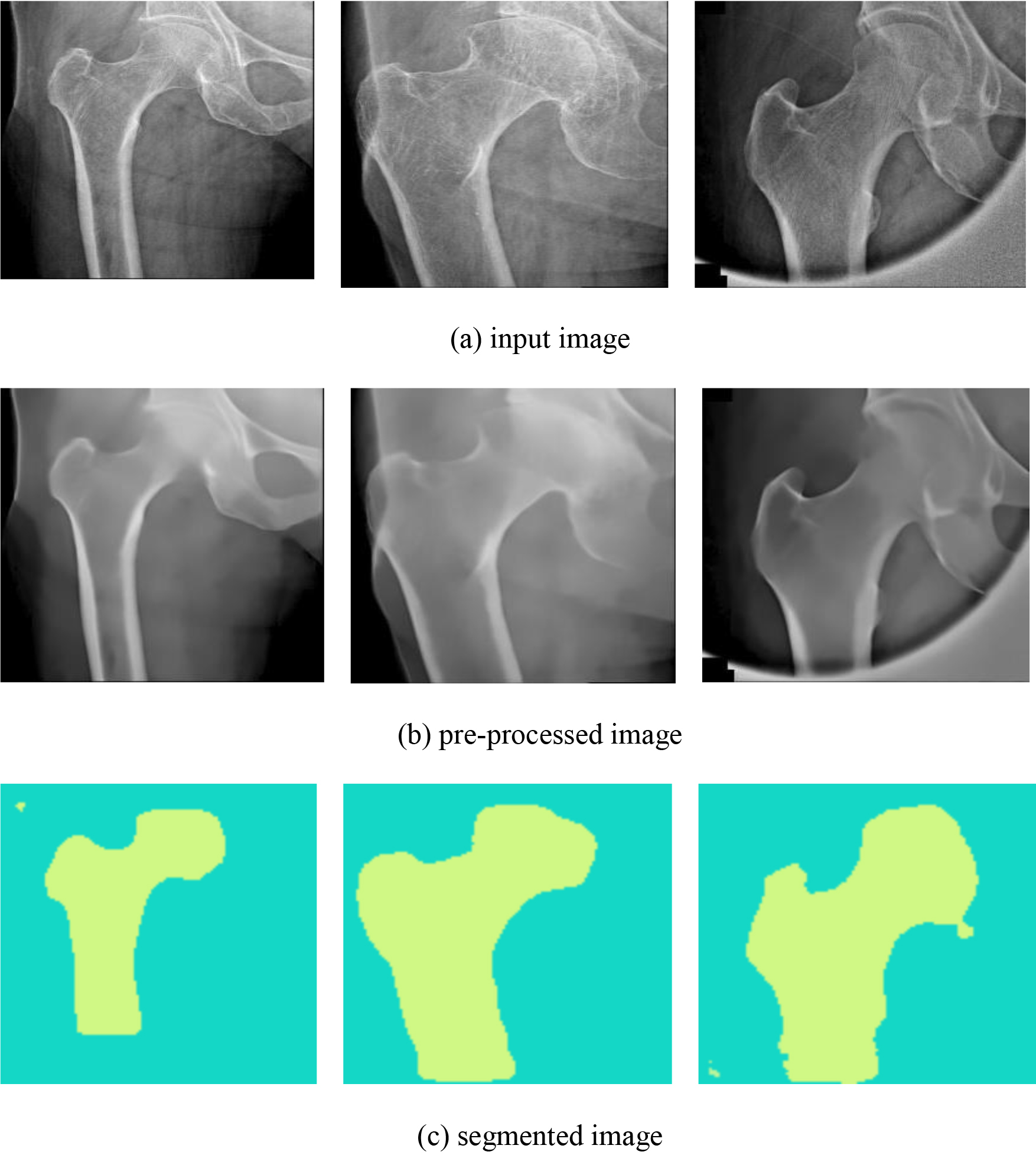

4.4 Evaluation metrics

The metrics including accuracy, PPV, NPV, TPR and TNR are considered to evaluate the performance of TJFO_DbneAlexNet in osteoporosis classification.

The accuracy metric exactly indicates the absence or presence of a disease among a whole quantity of samples analyzed.

$\displaystyle\textit{Accuracy}=\frac{TP+TN}{TP+TN+FP+FN}$ (32)

where $T P$ indicates true positive and $F P$ implies false positives. Also, $T N$ and $F N$ represents the true negative and false negative.

Positive Predictive Value (PPV) is a unit that verifies the presence of illness, in which the test predicts a positive outcome.

$\displaystyle\textit{PPV}=\frac{TP}{TP+FP}$ (33)

Negative Predictive Value (NPV) indicates a negative prediction and the person has a negative test result. It represents the absence of disease.

$\displaystyle\textit{NPV}=\frac{TN}{TN+FN}$ (34)

True Positive Rate (TPR) is utilized for identifying the ratio of diseased people who are precisely known as diseased. Moreover, the TPR is termed as sensitivity.

$\displaystyle\textit{TPR}=\frac{TP}{TP+FN}$ (35)

The fraction of precisely identifiable positive to overall negative results is demarcated as True Negative Rate (TNR). Furthermore, the TNR is indicated as,

$\displaystyle\textit{TNR}=\frac{TN}{TN+FP}$ (36)

4.5 Performance evaluation

Performance evaluation of the proposed TJFO_DbneAlexNet in several epochs are presented in Fig. 7. Here, accuracy, PPV, NPV, TPR and TNR are utilized for validating the performance of the proposed TJFO_DbneAlexNet. Furthermore, the performance is computed by modifying the training data. The performance evaluation regarding accuracy is depicted in Fig. 7a. For a training data of 70%, then the performance of TJFO_DbneAlexNet in 10, 20, 30, 40 and 50 epochs are 0.772, 0.794, 0.819, 0.827 and 0.876. Moreover, the performance of the proposed TJFO_DbneAlexNet in terms of PPV is shown in Fig. 7b. In 80% of training data, PPV of 0.801, 0.821, 0.843, 0.852 and 0.885 are achieved in 10, 20, 30, 40 and 50 epochs. Furthermore, Fig. 7c displays the assessment regarding to NPV. For 50% training data, the NPV of proposed TJFO_DbneAlexNet in 10 epoch is 0.702, 20 epoch is 0.731, 30 epoch is 0.750, 40 epoch is 0.785 and 50 epoch is 0.825. Similarly, the estimation regarding TPR is deliberated in Fig. 7d. Considering 60% training data, TPR values 0.745, 0.753, 0.765, 0.803 and 0.856 are attained in 10, 20, 30, 40 and 50 epochs. Similarly, the estimation of TNR is portrayed in Fig. 7e. Considering 90% training data, TNR of proposed TJFO_DbneAlexNet in 10, 20, 30, 40 and 50 epochs are 0.873, 0.889, 0.896, 0.904 and 0.933.

Figure 7.

Performance evaluation considering.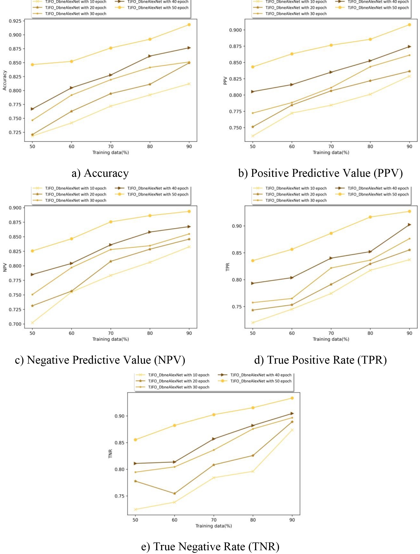

4.6 Comparative methods

The performance of the proposed TJFO_DbneAlexNet is compared to other existing methods like Mandibular Cortical Index and Mandibular Cortical Widths (MCI-MCW) [22], Recurrent Neural Network (RNN) [1], Convolutional Neural Network (CNN) [14] and CNN $+$ handcrafted features [18].

MCI-MCW: It uses the machine learning measurement software. It is performed using various tests for screening the osteoporotic condition. This method can achieve highly reproducible classification results.

RNN: It is widely used in orthopaedic studies and has the capability of producing better results in segmenting bone structure and osteoarthritis diagnosis. The best results are produced by this model in fracture prediction.

CNN: It has been used for examining osteoporosis and generates better results in detecting osteoporosis.

CNN $+$ handcrafted features: The CNN features have the capability of producing impressive results. Then merging of handcrafted features and CNN improves the accuracy of the model. This unification makes the model achieve unique characteristics in the field of osteoporosis research.

4.7 Comparative evaluation

The comparative assessment of the proposed TJFO_DbneAlexNet is explained by estimating metrics and modifying the K-fold and training data. Here, MCI-MCW, RNN, CNN and CNN $+$ handcrafted features are the existing methods considered for a comparative evaluation of TJFO_DbneAlexNet.

4.7.1 Estimation using training data

Comparative evaluation of TJFO_DbneAlexNet in osteoporosis classification using several training data is revealed in Fig. 8. Here, Fig. 8a shows the valuation corresponding to accuracy. Considering a training data of 70%, the accuracy of TJFO_DbneAlexNet is 0.883, while MCI-MCW, RNN, CNN and CNN $+$ handcrafted features got the accuracy of 0.749, 0.778, 0.797 and 0.844. Here, the performance increment of TJFO_DbneAlexNet compared to other methods is 15.08%, 11.91%, 9.740%, and 4.334%. The comparative estimation regarding to PPV is shown in Fig. 8b. In 50% of training data, PPV values 0.780, 0.800, 0.720, 0.760 and 0.836 are obtained by the MCI-MCW, RNN, CNN, CNN $+$ handcrafted feature proposed TJFO_DbneAlexNet. Therefore, proposed TJFO_DbneAlexNet achieved 6.643%, 4.308%, 13.83% and 9.076% of better performance. Additionally, the estimation related to NPV is portrayed in Fig. 8c. Here, MCI-MCW, RNN, CNN, CNN $+$ hand crafted feature and proposed TJFO_DbneAlexNet achieved the NPV of 0.716, 0.806, 0.812, 0.813 and 0.852 in 60% of training data. Therefore, 15.87%, 5.363%, 4.703% and 4.543% of enhanced performance is obtained by the proposed TJFO_DbneAlexNet. Similarly, Fig. 8d shows the comparative evaluation in terms of TPR. The proposed TJFO_DbneAlexNet obtained a TPR of 0.895 using 70% training data. Moreover, the TPR of MCI-MCW is 0.765, RNN is 0.866, CNN is 0.746 and CNN $+$ handcrafted feature is 0.796. Hence the TJFO_DbneAlexNet attained 14.45%, 3.191%, 16.66%, and 11.02% of performance increment with respect to others. Additionally, comparative evaluation by TNR is depicted in Fig. 8e, where the TNR of TJFO_DbneAlexNet is 0.873 for 60% of training data. Moreover, MCI-MCW, RNN, CNN and CNN $+$ handcrafted features provided the TNR of 0.739, 0.748, 0.782 and 0.0.808. Thus, the TJFO_DbneAlexNet achieved 15.37%, 14.24%, 10.35% and 7.443% of better performance when compared to the MCI-MCW, RNN, CNN and CNN $+$ handcrafted feature.

Figure 8.

Estimation using training data.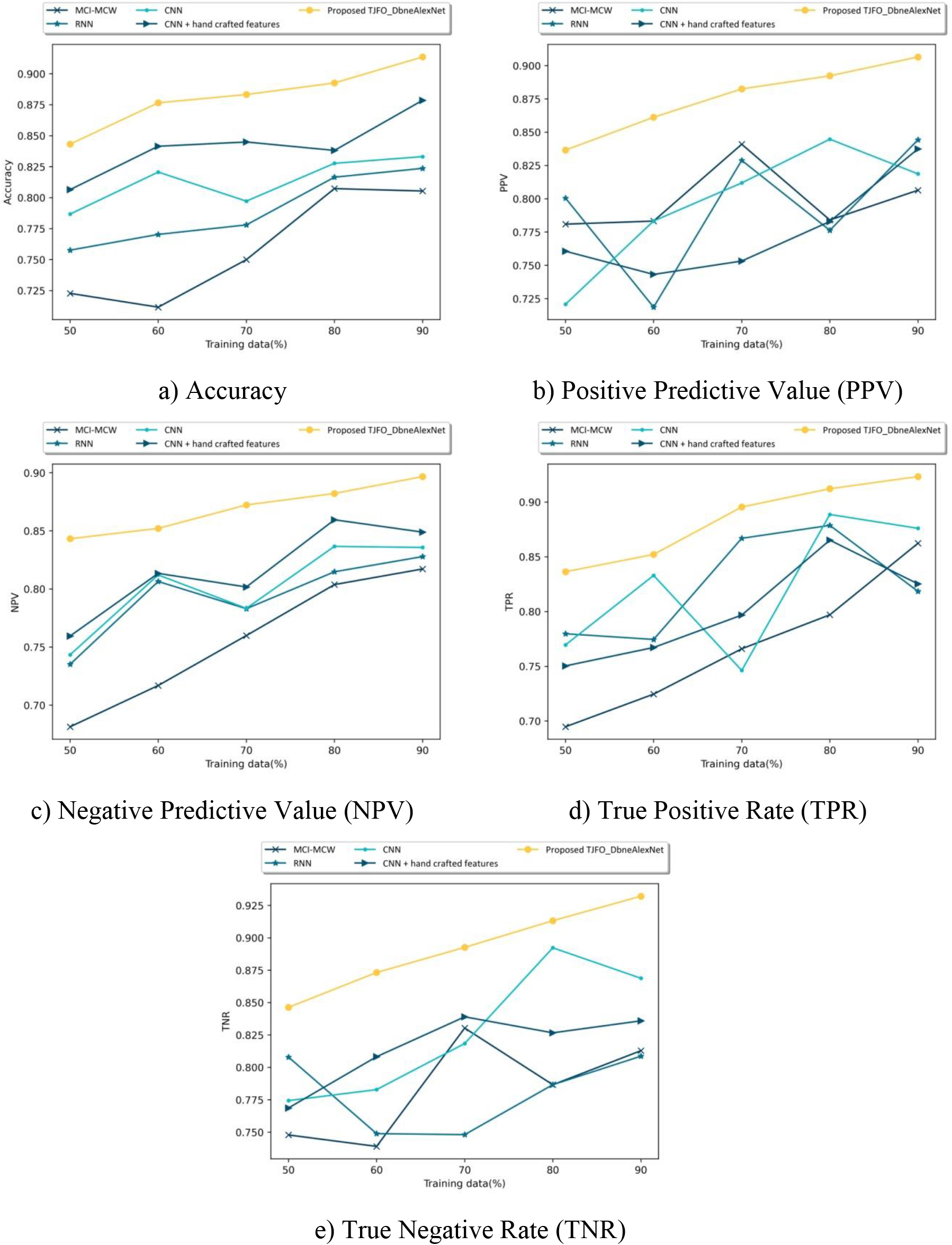

Figure 9.

Estimation using K-Fold.

4.7.2 Estimation using K-Fold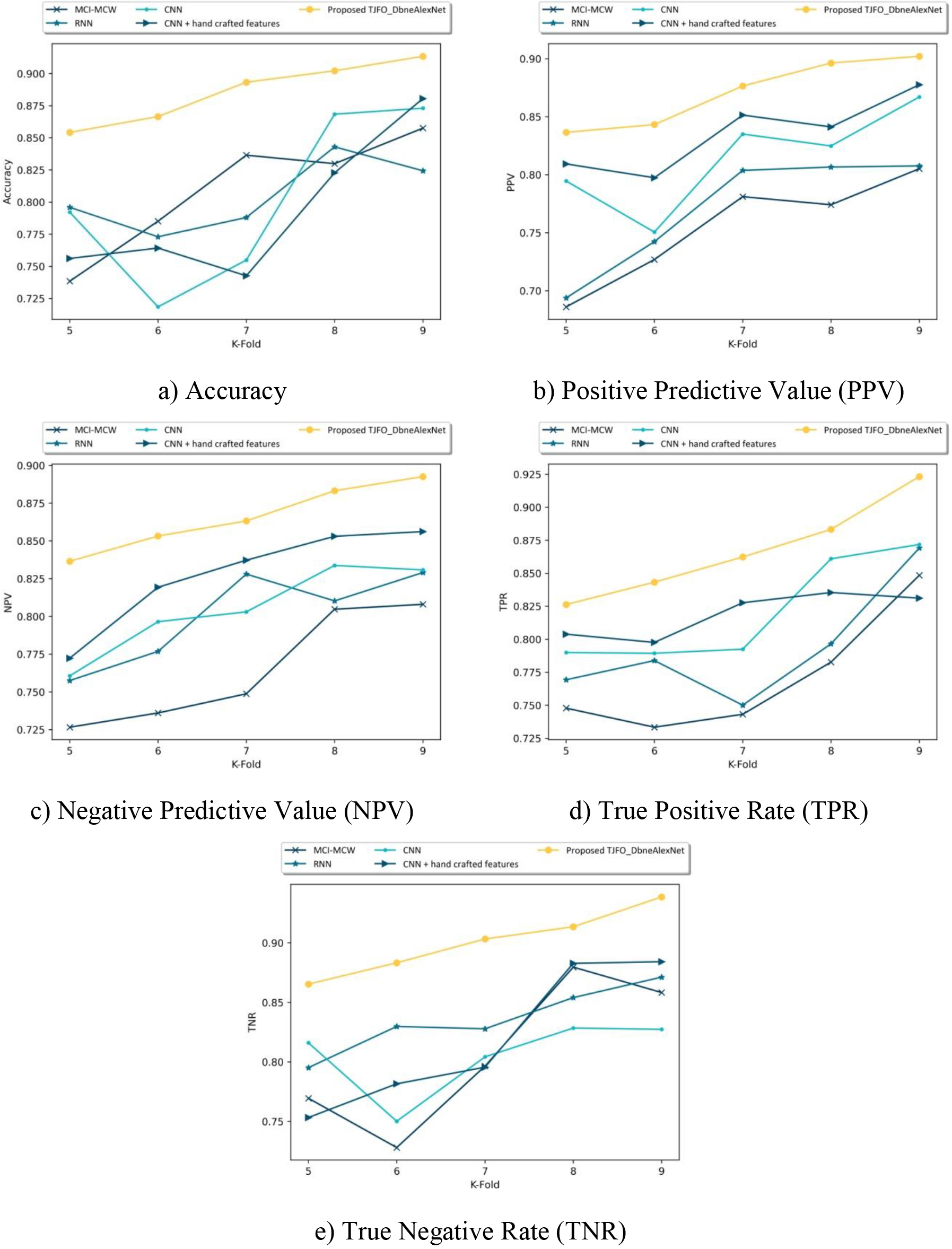

Figure 9 portrays the estimation of TJFO_DbneAlexNet in osteoporosis classification with regards to different K-Fold values. The assessment regarding accuracy is shown in Fig. 9a. Consider K-Fold $=$ 6, the accuracy of TJFO_DbneAlexNet is 0.866, in which the accuracy like 0.785, 0.773, 0.718, and 0.764 are got by MCI-MCW, RNN, CNN and CNN $+$ handcrafted feature. Hence, the TJFO_DbneAlexNet achieved 9.392%, 10.79%, 17.08%, and 11.80% of enhanced performance, while compared to MCI-MCW, RNN, CNN and CNN $+$ handcrafted features. The comparative assessment related to PPV is represented in Fig. 9b. For K-Fold $=$ 5, then the PPV of proposed TJFO_DbneAlexNet is 0.836, while the PPV of MCI-MCW is 0. 686, RNN is 0.693, CNN is 0.794 and CNN $+$ handcrafted feature is 0.809. Moreover, the performance increment of the proposed TJFO_DbneAlexNet to the other approaches is 17.98%, 17.06%, 5.013%, and 3.256%. Furthermore, the evaluation regarding to NPV is described in Fig. 9c. Consider K-Fold fold $=$ 7, the MCI-MCW, RNN, CNN, CNN $+$ handcrafted feature, and proposed TJFO_DbneAlexNet got the NPV like 0.748, 0.828, 0.803, 0.837, and 0.863. Thus, the proposed TJFO_DbneAlexNet has 13.26%, 4.078%, 6.975%, and 3.010% of better performance than other methodologies. In addition, Fig. 9d represents the assessment in connection with TPR values. Here, the proposed TJFO_DbneAlexNet achieved the TPR of 0.883 in K-Fold $=$ 8. Moreover, the TPR of MCI-MCW, RNN, CNN and CNN $+$ handcrafted features are 0.782, 0.796, 0.860 and 0.835. Furthermore, the TJFO_DbneAlexNet obtained 11.38%, 9.818%, 2.520%, and 5.417% of performance. In addition, the comparative estimation regarding TNR is deliberated in Fig. 9e. For K-Fold value $=$ 6, then the TNR of TJFO_DbneAlexNet is 0.883, while the TNR of MCI-MCW is 0.728, RNN is 0.829, CNN is 0.750 and CNN $+$ handcrafted feature is 0.781. From these values, the TJFO_DbneAlexNet has 17.55%, 6.047%, 15.06%, and 11.50% of an improved performance improvement than MCI-MCW, RNN, CNN and CNN $+$ handcrafted feature.

4.8 Comparative discussion

Table 2 denotes a comparative discussion of the performance of the proposed TJFO_DbneAlexNet and existing approaches. Here, the performance of TJFO_DbneAlexNet and the existing methodologies are attained in numerous K-Fold and training data. In 90% of training data, the maximum accuracy of the proposed TJFO_DbneAlexNet is 0.913, whereas MCI-MCW, RNN, CNN and CNN $+$ handcrafted feature has an accuracy of 0.805, 0.823, 0.833 and 0.878. Moreover, a greater PPV of 0.906 is obtained by the proposed TJFO_DbneAlexNet, while the PPV of existing methods are 0.806, 0.844, 0.818, and 0.837. Furthermore, the NPV of the proposed TJFO_DbneAlexNet is 0.896, whereas MCI-MCW, RNN, CNN and CNN $+$ handcrafted features attained the NPV of 0.817, 0.827, 0.835 and 0.848. Similarly, the superior TPR of the proposed TJFO_DbneAlexNet is 0.923. Here the TPR of MCI-MCW is 0.862, RNN is 0.818, CNN is 0.875 and CNN $+$ handcrafted feature is 0.825. Likewise, the proposed TJFO_DbneAlexNet has the superior TNR of 0.932, while the TNR of MCI-MCW, RNN, CNN and CNN $+$ handcrafted features are 0.812,0.808, 0.868 and 0.835. For different K-Fold values, the accuracy, PPV, NPV, TPR and TNR of TJFO_DbneAlexNet are 0.913, 0.902, 0.892, 0.923 and 0.938. It is noticed that the finest results are obtained in training data variation.

Table 2
Comparative discussion

Variations	Metrics	MCI-MCW	RNN	CNN	CNN $+$ handcrafted feature	Proposed TJFO_DbneAlexNet
Training data (90%)	Accuracy	0.805	0.823	0.833	0.878	0.913
	PPV	0.806	0.844	0.818	0.837	0.906
	NPV	0.817	0.827	0.835	0.848	0.896
	TPR	0.862	0.818	0.875	0.825	0.923
	TNR	0.812	0.808	0.868	0.835	0.932
K-Fold values (9)	Accuracy	0.857	0.824	0.873	0.880	0.913
	PPV	0.805	0.807	0.867	0.877	0.902
	NPV	0.808	0.829	0.830	0.856	0.892
	TPR	0.848	0.869	0.871	0.831	0.923
	TNR	0.868	0.871	0.827	0.884	0.938

Figure 10.

Confusion matrix.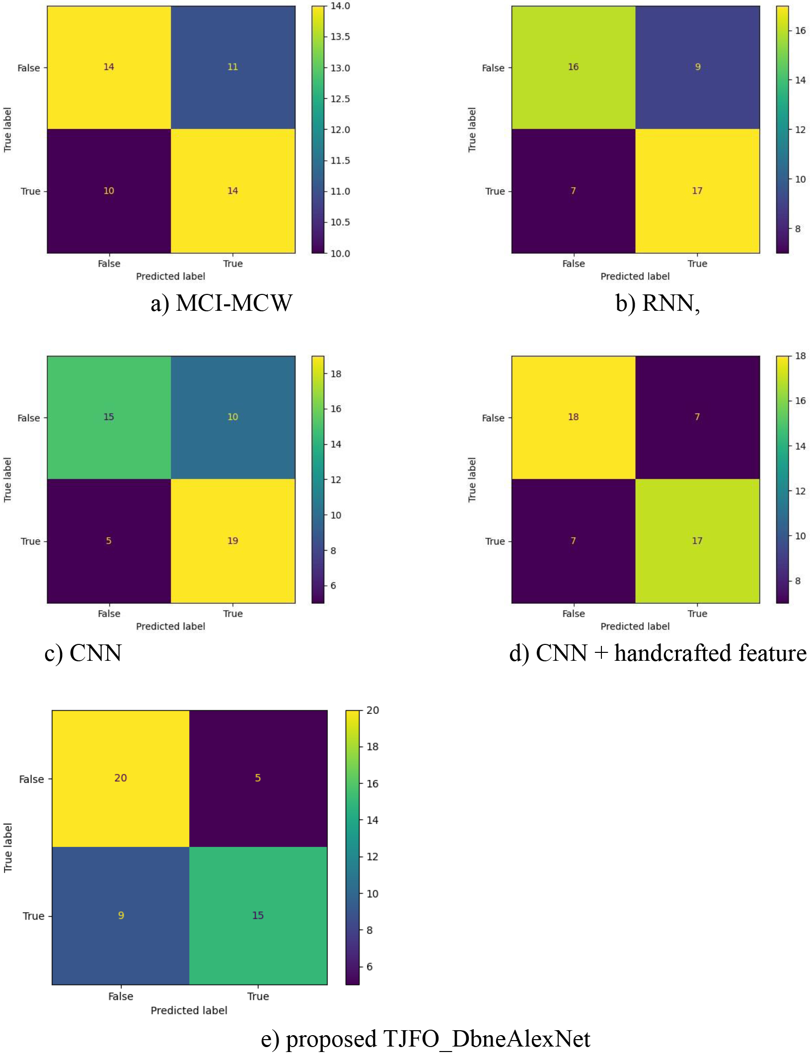

Figure 11.

Convergence curve of the proposed TJFO_DbneAlexNet.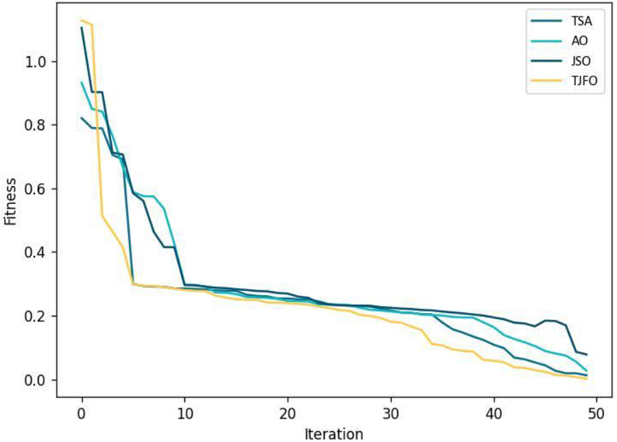

4.9 Confusion matrix

In certain systems, the collection of the predicted and actual classification information is called a confusion matrix. Figure 10a–d, and e specifies the confusion matrix of the MCI-MCW, RNN, CNN, CNN $+$ handcrafted feature, and proposed TJFO_DbneAlexNet. The confusion square matrix is created in the predictive analysis phase that contains positive and negative rates (both true and false). The x-axis represents the predicted label classes and the y-axis shows the true label classes.

4.10 Convergence plots

The value of the objective function against the computation time during the minimization process is shown using the convergence curve. Figure 11 shows the convergence behavior of the proposed method. The algorithms used for comparison are the Tunicate Swarm Algorithm (TSA) [20], Aquila Optimizer (AO) [12], Jellyfish search optimization (JSO) [8], and the proposed TJFO. The fitness values obtained by the TSA, AO, JSO, and TJFO are 0.0134, 0.0277, 0.787, and 0.0022 for iteration 50. The evaluation results show that the proposed method can converge more easily than the other methods.

5. Conclusion

In the medical field, osteoporosis is a silent killer disease associated with the danger of fractures, which is often diagnosed based on T-score and Bone Mineral Density (BMD) values. Generally, osteoporosis is a bone condition that includes reduced bone mass, bone degeneration on a lesser scale and a high tendency to fracture. It is a significant prosperity stress throughout the world. Thus, the deep learning based osteoporosis classification is modelled in this research. Furthermore, an X-ray image of the femur bones is used in the osteoporosis classification. The Non-Local Means (NLM) filter is applied to diminish the noise of input bone images. The SegNet is used to isolate certain parts of an image during the segmentation process. After measuring the femur geometry, the medical, GLCM, LVP, CNN and PHoG features are extracted. The tuna jellyfish optimization trained DbneAlexNet is used for osteoporosis classification. Furthermore, the efficiency of the proposed model is valued by the accuracy, PPV, NPV, TPR and TNR measures, where the optimum values such as 0.913, 0.906, 0.896, 0.923, and 0.932 are attained. In future, this framework will be enhanced through a hybrid network model to attain ever more superior performance.

Footnotes

Author’s Bios

Halesh T G ORCID: 0009-0006-7770-6564. I have completed my MSc, in Computer Science from Kuvempu University Shankaraghatta, in the year 2004 and completed my MPhil from Kuvempu University Shankaraghatta, in the year 2008, My area of research was Image processing in MR-Images, Currently working as Assistant Professor at Smt. Indira Gandhi Government First Grade Women’s college, Sagar and percuing PhD from CMR University, Bangalore the area of research in Image Processing and Machine Learning. I completed my BSc in Computer Science from SRNMC college Shimoga affiliated to Kuvempu University.

P. Sathish received his doctoral degree (Ph.D) (2021) in computer science and master degree (MCA) (2009) from Bharathiar University, Tamilnadu, India and M.Phil (2011) from PRIST University, Tanjore, Tamilnadu, India. He received his undergraduate degree (B.Sc) in Mathematics (2006) from Periyar University, Tamilnadu, India. Currently, he is working as an Associate Professor, School of Science Studies, CMR University, Bangalore. He has 13 years of teaching and 1 year of industry experience. His area of expertise includes Image Processing, Machine Learning and Data Mining. He received one patent grant from Australian Innovation Patent in the year 2021 and published two Indian patents in the year 2022. He published six research papers in the field of medical image processing in SCIE, Scopus and UGC journals. He presented more than 10 research papers in the national and international conferences. He is the technical reviewer of various international journals.

References

Shaker

A.S.

, Detection and segmentation of osteoporosis in human body using recurrent neural network, International Journal of Advanced Science and Technology 29(02) (2020), 1055–1066.

Zhang

Ning

Wang

Dong

Liu

Wang

Zhu

and Duan

, Deep learning of lumbar spine X-ray for osteopenia and osteoporosis screening: A multicenter retrospective cohort study, Bone 140 (2020), 115561.

Hemanth

D.J.

and Anitha

, Image pre-processing and feature extraction techniques for magnetic resonance brain image analysis, in: International Conference on Future Generation Communication and Networking, Springer, Berlin, Heidelberg, 2012, pp. 349–356.

Alaeddine

and Jihene

, Deep Batch-normalized eLUAlexNetFor Plant Diseases Classification, in: Proceedings of 18th International Multi-Conference on Systems, Signals & Devices (SSD), 2021, pp. 17–22.

Liu

Wang

Ruan

Lin

and Chen

, Diagnostic and gradation model of osteoporosis based on improved deep U-Net network, Journal of Medical Systems 44(1) (2020), 1–7.

Kemp

J.P.

Morris

J.A.

Medina-Gomez

Forgetta

Warrington

N.M.

Youlten

S.E.

Zheng

Gregson

C.L.

Grundberg

Trajanoska

and Logan

J.G.

, Identification of 153 new loci associated with heel bone mineral density and functional involvement of GPC6 in osteoporosis, Nature Genetics 49(10) (2017), 1468–1475.

Chou

J.S.

and Truong

D.N.

, A novel metaheuristic optimizer inspired by behavior of jellyfish in ocean, Applied Mathematics and Computation 389 (2021), 125535.

Chou

J.S.

and Truong

D.N.

, A novel metaheuristic optimizer inspired by behavior of jellyfish in ocean, Applied Mathematics and Computation 389 (2021).

Xia

Yin

Qian

Jiang

and Wang

, Liver semantic segmentation algorithm based on improved deep adversarial networks in combination of weighted loss function on abdominal CT images, IEEE Access 7 (2019), 96349–96358.

10.

Fan

K.C.

and Hung

T.Y.

, A novel local pattern descriptor – local vector pattern in high-order derivative space for face recognition, IEEE Transactions on Image Processing 23(7) (2014), 2877–2891.

11.

Xia

K.J.

Yin

H.S.

and Zhang

Y.D.

, Deep semantic segmentation of kidney and space-occupying lesion area based on SCNN and ResNet models combined with SIFT-flow algorithm, Journal of Medical Systems 43(1) (2019), 1–12.

12.

Abualigah

Yousri

Elaziz

M.E.A.

and Ewees

A.A.E.

, Aquila Optimizer: A novel meta-heuristic optimization Algorithm, Computers and Industrial Engineering 157(11) (2021).

13.

Xian

Han

Zhou

Zhang

Z.R.

Han

and Tang

, Tuna swarm optimization: a novel swarm-based metaheuristic algorithm for global optimization, Computational intelligence and Neuroscience, 2021.

14.

Shahzad

Khan

T.F.

Bashir

Ayub

Ashraf

Hashmi

Zahoor

and Jaskani

F.H.

, Detection of osteoporosis in defected bones using RADTorch and deep learning techniques, International Journal of Engineering Applied Sciences and Technology 6(4) (2021), 2455–2143.

15.

Khairandish

M.O.

Sharma

Jain

Chatterjee

J.M.

and Jhanjhi

N.Z.

, A hybrid CNN-SVM threshold segmentation approach for tumor detection and classification of MRI brain images, Irbm 43(4) (2022), 290–299.

16.

Shankar

Babu

S.S.

and Viswanathan

, Femur bone volumetric estimation for osteoporosis classification using optimization-based deep belief network in X-ray images, The Computer Journal 62(11) (2019), 1656–1670.

17.

Dzierzak

and Omiotek

, Application of deep convolutional neural networks in the diagnosis of osteoporosis, Sensors 22(21), 8189.

18.

Liu

Sun

Jin

Jennane

and Wei

, Fusing convolutional neural network features with hand-crafted features for osteoporosis diagnoses, Neurocomputing 385 (2020), 300–309.

19.

Chachada

B.T.

Cho

Phong

S.A.

Manchala

and Kuo

C.C.J.

, Extension of Non-Local Means (NLM) algorithm with Gaussian filtering for highly noisy images, In Visual Communications and Image Processing (VCIP), 2011, 1–4.

20.

Kaur

Awasthi

L.K.

Sangal

A.L.

and Dhiman

, Tunicate Swarm Algorithm: A new bio-inspired based metaheuristic paradigm for global optimization, Engineering Applications of Artificial Intelligence 90 (2020).

21.

Fathima

S.M.N.

Tamilselvi

Beham

M.P.

and Sabarinathan

, Diagnosis of osteoporosis using modified U-net architecture with attention unit in DEXA and X-ray images, Journal of X-Ray Science and Technology 28(5) (2020), 953–973.

22.

Suzuki

Katsumata

Mastumoto

Komatu

Oomura

Okamura

Mizuno

Anazawa

and Nomura

, Features of mandibular cortical bone morphology in osteoporotic fracture patients, Oral Radiology, 2022, 1–8.

23.

Mughal

Khawaja

H.A.

and Moatamedi

, Finite element analysis of human femur bone, 2015.

24.

Prakash

U.M.

Kottursamy

Cengiz

Kose

and Hung

B.T.

, 4x-expert systems for early prediction of osteoporosis using multi-model algorithms, Measurement 180 (2021), 109543.

25.

Badrinarayanan

Kendall

and Cipolla

, Segnet: A deep convolutional encoder-decoder architecture for image segmentation, IEEE Transactions on Pattern Analysis and Machine Intelligence 39(12) (2017), 2481–2495.

26.

Bai

Guo

Jin

and Huang

, A novel feature extraction method using pyramid histogram of orientation gradients for smile recognition, in: Proceedings of 16th IEEE International Conference on Image Processing (ICIP), 2009, pp. 3305–3308.

27.

Fang

Chen

Kang

Zhang

Liao

Hong

and Li

, Opportunistic osteoporosis screening in multi-detector CT images using deep convolutional neural networks, European Radiology 31(4) (2021), 1831–1842.

28.

Jiang

Chung

F.L.

Ishibuchi

Deng

and Wang

, Multitask TSK fuzzy system modeling by mining intertask common hidden structure, IEEE Transactions on Cybernetics 45(3) (2014), 534–547.

29.

Jiang

Chung

F.L.

Wang

Deng

Wang

and Qian

, Collaborative fuzzy clustering from multiple weighted views, IEEE Transactions on Cybernetics 45(4) (2014), 688–701.

Femur bone volumetric estimation for osteoporosis classification based on deep learning with tuna jellyfish optimization using X-ray images

Abstract

Keywords

1. Introduction

1.1 Motivation

1.2 Main contribution

1.3 Structural organization

2. Literature review

2.1 Major challenges

3. Proposed tuna jellyfish optimization based DbneAlexNet for osteoporosis classification

3.4 Femur geometry measurement

3.5.1 Grey level co-occurrence matrix (GLCM) texture features

3.5.3 Local Vector Pattern (LVP) feature

3.6.1 Architecture of DbneAlexNet

4.1 Experimental setup

Table 1 Experimental parameters of the proposed TJFO_DbneAlexNet model

4.3 Dataset description

4.7 Comparative evaluation

4.7.1 Estimation using training data

4.8 Comparative discussion

Table 2 Comparative discussion

4.10 Convergence plots

5. Conclusion

Footnotes

Author’s Bios

References

Table 1
Experimental parameters of the proposed TJFO_DbneAlexNet model

Table 2
Comparative discussion