Sage Journals: Discover world-class research

Abstract

A criterion is proposed for testing the hypothesis about the nature of the error variance in the dependent variable in a linear model, which separates correctly and incorrectly specified models. In the former one, only the measurement errors determine the variance (i.e., the dependent variable is correctly explained by the independent ones, up to measurement errors), while the latter model lacks some independent covariates (or has a nonlinear structure). The proposed MEMV (Measurement Error Model Validity) test checks the validity of the model when both dependent and independent covariates are measured with errors. The criterion has an asymptotic character, but numerical simulations outlined approximate boundaries where estimates make sense. A practical example of the test’s implementation is discussed in detail – it shows the test’s ability to detect wrong specifications even in seemingly perfect models. Estimations of the errors due to the omission of the variables in the model are provided in the simulation study. The relation between measurement errors and model specification has not been studied earlier, and the proposed criterion may stimulate future research in this important area.

Keywords

Measurement errors linear regression model misspecification Wald test causality models adjusted least squares variables omission

1. Introduction

Consider a typical model, so often to be found in different versions in statistical literature:

$\displaystyle y=c_{1}x_{1}+c_{2}x_{2}+\ldots+e$ (1)

where $x$ are covariates (explanatory or independent variables); $y$ is the response (dependent) variable; $c$ are the “actual parameters” to be estimated; $e$ is the error term. There are many interpretations of such linear models and, respectively, ways to make estimates. In (Kukush & Mandel, 2019) we considered 16 different scenarios, where assumptions about measurements with or without errors and causal and non-causal interpretations of the coefficients were combined. And still, those combinations do not cover the other aspects of modeling, such as “endogenous” and “exogenous” variables; “latent and observable” variables; normal errors distributions or not; homoskedasticity, etc. So, the “simple” Eq. (1) becomes too complicated under exact specifications.

It is enough to say, that one cannot realistically assume that anything could be measured without errors – and yet this assumption prevails in all statistical literature, in standard statistical textbooks, and even in specialized volumes for linear models like in (Agresti, 2015). Similarly, statistical books and articles usually do not use causal terminology, while very developed causality modeling works (Pearl, 2009; Morgan, 2014) tend to consider the coefficients $c$ , obtained by usual regression as causal only because those regressions are embedded into a special framework (directed acyclic graphs). However, it does not make them by default causal, as shown in detail in (Mandel, 2017, 2018). There is a corpus of works for causal discovery in observational data (Peters et al., 2017; Janzing & Schölkopf, 2018; Glymor et. al., 2019), and some part of it is related to errors in variables; recently this literature was reviewed for the first time by Linda Valeri in (Yi et. al., eds., 2021), but it is far from being an established part of the statistical toolkit.

Among many problems let us focus on one – on the interpretation of the so-called random term $e$ in Eq. (1). Technically, it looks like a value needed to be added to the deterministic term of the equation $c^{T}x$ to be equal to the $y$ value precisely (or, in backward interpretation, as “residual” when Y is already estimated). Neither the nature of that addition nor the reason for its appearance is usually considered. It is just assumed, that some difference always exists and one needs to minimize it (the whole idea of LS and all other methods is exactly that). Typically, it is considered as some kind of construction with convenient features, like this: $e_{i}$ “…are independent and identically distributed random variables with zero mean and constant variance” (Demidenko, 2004, p. 3).

This type of treatment of those “residuals” holds a key question about their nature unanswered. Say, if two covariates should determine $y$ , but we have in a model just one of them, then the interpretation and assumption about i.i.d. in literature will not change. Equally, if suddenly the third (unnecessary) covariate is included in a model (with spoiling effect) – the interpretation, again, will be as it is. But the crucial difference is that only when two causal variables are in a model, $e$ becomes a pure error of measurement, while in any misspecification it is not true. One somehow should distinguish between errors due to misspecification and due to mismeasurement. The lack of clarity in this question is a strong contributor to the sad situation of the “reproducibility crisis” (Baker, 2016) and “statistical significance crisis” (Wasserstein & Lazar, 2016; Amrhein et al., 2019), in our opinion.

Despite awareness of that type for a long time, the new studies confirm, that statistics remains not a reliable tool for the actual researchers. Gould et al. (2023) have convincingly shown that even if many specialists (more than 200) receive the same set of biological and environmental data, which have no political or ideological connotation (to avoid easily expected biases), the conclusions could be vastly different. Such an experiment was done for the first time and was different from the earlier ones when multiple groups tried to reproduce the conditions of the original study. In that study, with the same data sets, only statistical tools and the researcher’s imagination played a role. Unfortunately, the authors of this mega study did not provide the exact reasons for the results differentiation (like one used this criterion, another – another one, etc.), and we cannot say for sure, what exactly happened, but it is clear that “the standard statistical treatment” was not in place, with gradual drifting of the estimates of the effect from positive to negative. In the same vein, we do not know how researchers accounted for measurement errors if they did. All that raises profound questions about the level of confidence society should have about the typical statistical study.

The misspecification error alone could be very significant, as shown in Section 3. However, the main focus of the paper is to analyze the effect of the measurement errors on the conclusion about the quality of the Eq. (1). We try to deal with just one question: in what case one may say with confidence, that the built model does not reflect just measurement errors but measures something more substantial. Or, in other words, having any idea about the possible level of the measurement errors in the data – can one say, that the model captures strong (not necessarily causal) relations between variables, which are not hidden by measurement errors? Such situations are technically related to the so-called equation error model (see Section 1.5 in (Kukush, 2011)).

The proposed criterion we named MEMV (Measurement Error Model Validity) test, for it distinguishes valid (i.e., complete) models where only inevitable measurement errors play a role, and invalid (incomplete) models, where hidden covariates (not included in a model) affect the variance of the independent covariate. Moreover, even in a complete model, the test rejects the validity hypothesis when assumed errors in covariates are too high. The test allows, more specifically, answering the following question: is the quality of the model (say, coefficient of determination or another indicator) higher than the level that could be obtained just by accounting for the measurement errors? If yes, then the model makes sense; if no – it does not, regardless of its goodness-of-fit level. This type of criterion could be very useful in situations, where a researcher has a plausible idea about the level of measurement errors either for $y$ or for $x$ , or just knows for sure about it (when, for example, the precision of the measurement devices is accessible). In a certain sense, it inverses the usual formulation of the errors in variables problem: how to adjust the coefficients of regression to account for measurement errors of different types (Kukush, 2011; Schennach, 2016; Yi et al., 2021). In this latter scenario, one gets the estimates with wider confidence intervals, but still believes that she found “something”. In the former scenario, one knows that nothing good could be expected if the model covers just errors and (erroneously) the hidden factors and nothing more.

The rest of the article is organized as follows. Section 2 describes a specific case of Eq. (1), where the covariates $x$ are observed with additive measurement error; in our approach, the variance $\sigma^{2}=\textit{Var}(e)$ is a parameter of interest and $c$ plays a role of nuisance parameter (unlike under usual treatment); based on the assumption of the independent observations, we constructed a consistent and asymptotically normal estimator of $\sigma^{2}$ , that yields a one-sided Wald test which serves as a desired criterion for the separation of the correctly and incorrectly specified models. Section 3 contains the results of the simulation experiment. Section 4 demonstrates how to implement the test on the real data and presents some non-trivial results; Conclusion summarizes the main results and outlines the area of future research. Appendix 1 contains proofs of the asymptotic properties of the estimators; Appendix 2 studies the behavior of the test for large sample size and the growing level of the presumed measurement errors.

All the vectors in the paper are column ones. Abbreviation r.v. means random variable; Var stands for the variance of a r.v. and Cov for the variance-covariance matrix of a centered random vector.

2. Hyrothesis testing concerning the error variance

2.1 Basic regression model

We deal with a linear functional errors-in variables model

$\displaystyle y=c^{T}x+e,$ (2) $\displaystyle w=x+\delta.$ (3)

Here $x$ is a nonrandom vector of covariates; $y$ is an observable response variable; $\delta$ is a vector of measurement errors; $e$ is another error term that may appear not only as a result of measurement, but as an effect of misspecification (e.g., lack or of covariates actually affecting $y$ ); instead of true covariates $x$ , we observe a surrogate data $w$ ; $c$ is a vector of unknown regression parameter, and $c^{T}$ is the vector transposed.

Concerning error terms, we assume the following.

(i)

The error $e$ in response is a centered r.v., and the measurement error $\delta$ in covariates is a centered random vector; moreover, $e$ and $\delta$ are independent with finite 2nd moments.

(ii)

The error variance $\sigma^{2}:=\textit{Var}(e)$ is not vanishing and unknown, while the measurement error covariance matrix $S:=\textit{Cov}(\delta)$ is known, where $S$ is a positive semidefinite matrix (see Remarks below for more detail).

Remark 1. It is allowed that some components $\delta^{(j)}$ of $\delta$ have zero variance. Thus, a subgroup of covariates can be observed without measurement error.

Remark 2. In practice, sometimes $S$ can be reliably estimated by repeated measurements of covariates. Another possible case is as follows: components of $\delta$ are independent and $S=\textit{diag}({\tau_{1}^{2},\ldots,\tau_{m}^{2}})$ with $\tau_{j}^{2}=\textit{Var}({\delta^{(j)}})$ known from the passport information of measurement devices. In case $S=0,$ we have the ordinary linear regression Eq. (2) with both observable $y$ and $x$ .

Remark 3. Other possible cases of available information concerning $\sigma^{2}$ and $S$ will be indicated in Conclusion. Note that some information about the error covariance structure should be available, otherwise the Eqs (2) and (3) is not identifiable, and in that case even for Gaussian errors it is impossible to estimate all the model parameters consistently as the sample size tends to infinity (Chen & Van Ness, 1999).

Individual observations in a data set are modeled as independent copies of the basic model

$\displaystyle y_{i}=c^{T}x_{i}+e_{i},$ (4) $\displaystyle w_{i}=x_{i}+\delta_{i},i=1,\ldots,n.$ (5)

Here $x_{1},\ldots,x_{n}$ are nonrandom and unknown vectors; $\{e_{i},i\geqslant 1\}$ are independent i.i.d. random values distributed as $e$ in the Eqs (2) and (3), $\{\delta_{i},i\geqslant 1\}$ are i.i.d. random vectors distributed as $\delta$ , and the two sequences are assumed mutually independent; $n$ – number of observations. Based on observations

$\displaystyle({y_{1},w_{1}}),\ldots,(y_{n},w_{n}),$ (6)

we want to estimate $\sigma^{2}=\textit{Var}(e)$ and test a hypothesis that its value does not exceed a fixed level.

2.2 Consistent estimators of model parameters

As a consistent estimator of $c$ , we use the so-called adjusted least squares (ALS) estimator (Cheng & Van Ness, 1999):

$\displaystyle\hat{c}=({\overline{ww^{T}}-S})^{+}\overline{wy}.$ (7)

Hereafter, the bar stands for averaging over the whole sample, in particular $\overline{ww^{T}}:=\frac{1}{n}\mathop{\sum}\limits_{i=1}^{n}w_{i}w_{i}^{T}$ , $\overline{wy}=\frac{1}{n}\mathop{\sum}\limits_{i=1}^{n}w_{i}y_{i}$ ; $D^{+}$ denotes the pseudo-inverse matrix of a matrix $D$ . If the matrix $\overline{ww^{T}}-S$ is nonsingular, then Eq. (7) takes a form

$\displaystyle\hat{c}=({\overline{ww^{T}}-S})^{-1}\overline{wy},$ (8)

where $D^{-1}$ is the inverted matrix. Under mild assumptions this happens with probability tending to 1 as $n\to\infty$ (see statement 1 of Theorem in Appendix 1).

A consistent estimator $\tilde{\sigma}^{2}$ of $\sigma^{2}$ is based on the following computation:

$\displaystyle E({y-c^{T}w})^{2}=E({e-c^{T}\delta})^{2}=\sigma^{2}+c^{T}Sc.$ (9)

Thus, $\tilde{\sigma}^{2}$ is expressed through the residual sum of squares $\textit{RSS}:=\mathop{\sum}\limits_{i=1}^{n}({y_{i}-\hat{c}^{T}w_{i}})^{2}$ ,

$\displaystyle\tilde{\sigma}^{2}:=n^{-1}\textit{RSS}-\hat{c}^{T}S\hat{c}.$ (10)

Let us introduce estimating functions

$\displaystyle s_{c}=s_{c}({y,w;c})=wy-({ww^{T}-S})c,$ (11) $\displaystyle s_{\sigma^{2}}=s_{\sigma^{2}}({y,w;c,\sigma^{2}})=({y-c^{T}w})^{% 2}-c^{T}Sc-\sigma^{2}.$ (12)

With probability tending to 1 as $n\to\infty$ , the pair $(\hat{c};\tilde{\sigma}^{2})$ is a solution to the estimating equations

$\displaystyle\mathop{\sum}\limits_{i=1}^{n}s_{c}(y_{i},w_{i};c)=0,\mathop{\sum% }\limits_{i=1}^{n}s_{\sigma^{2}}(y_{i},w_{i};c,\sigma^{2})=0,c\epsilon R^{m},% \sigma^{2}\geqslant 0.$ (13)

The estimator Eq. (10) is consistent, i.e. $\tilde{\sigma}^{2}$ converges in probability to $\sigma^{2}>0$ as $n\to\infty$ (see Appendix 1). Hence the right-hand side of Eq. (10) is positive with probability tending to 1. For finite sample, it can happen that $n^{-1}\textit{RSS}-\hat{c}^{T}S\hat{c}<0$ , and we modify the estimator Eq. (10) as follows

$\displaystyle\hat{\sigma}^{2}:=\max(0,\tilde{\sigma}^{2})=\max(0,n^{-1}\textit% {RSS}-\hat{c}^{T}S\hat{c}).$ (14)

2.3 Asymptotic normality of the estimators and Wald test

Let us denote the following vector of parameters:

$\displaystyle\theta=({c^{T};\sigma^{2}})^{T},\hat{\theta}=(\hat{c}^{T};\hat{% \sigma}^{2})^{T}.$ (15)

The corresponding unbiased estimating vector function is as follows

$\displaystyle s_{\theta}=s_{\theta}({y,w;\theta})=({s_{c}^{T};s_{\sigma^{2}}})% ^{T},$ (16)

where the components $s_{c}$ and $s_{\sigma^{2}}$ are given in Eqs (11) and (12). The estimating equation for $\hat{\theta}$ is

$\displaystyle\mathop{\sum}\limits_{i=1}^{n}s_{\theta}(y_{i},w_{i};\theta)=0,% \theta\epsilon R^{m}\times[{0,\infty}).$ (17)

Actually, $\hat{\theta}$ is a Borel function of observations $y_{1},w_{1},\ldots,y_{n},w_{n}$ such that $\hat{\theta}$ is a solution to Eq. (17) if it has a solution. Under the corresponding model assumptions, the Eq. (17) has a solution with probability tending to 1 as $n\to\infty$ (see Appendix 1).

Under a bit stronger model assumption, the estimator $\hat{\theta}$ is consistent (i.e. $\hat{\theta}$ converges to true $\theta$ in probability as $n\to\infty$ ) and asymptotically normal. Sufficient conditions for the consistency and asymptotic normality of $\hat{\theta}$ are given in Appendix 1. They include finiteness of error moments of some order greater than 4, convergence of sample means of $x$ up to 4th order, and non-singularity of the matrix

$\displaystyle\mu_{2}:=\lim_{n\to\infty}\frac{1}{n}\mathop{\sum}\limits_{i=1}^{% n}x_{i}x_{i}^{T}.$ (18)

The asymptotic covariance matrix $\Sigma_{\theta}$ can be found from the sandwich formula (Carrol et al., 2006):

$\displaystyle\Sigma_{\theta}=A^{-1}BA^{-T},$ (19) $\displaystyle A:=-\lim_{n\to\infty}\frac{1}{n}\mathop{\sum}\limits_{i=1}^{n}E% \frac{\partial s_{\theta}({y_{i},w_{i}})}{\partial\theta^{T}},B:=\lim_{n\to% \infty}\frac{1}{n}\mathop{\sum}\limits_{i=1}^{n}Es_{\theta}({y_{i},w_{i}})s_{% \theta}^{T}({y_{i},w_{i}}).$ (20)

Here $A^{-T}:=({A^{-1}})^{T}$ and the functions are evaluated at the true point $\theta$ . We assume that $B$ is nonsingular, and therefore, $\Sigma_{\theta}$ is nonsingular as well. In our case, $A$ is symmetric, hence $A^{-T}=A^{-1}$ and Eq. (19) takes a form

$\displaystyle\Sigma_{\theta}=A^{-1}BA^{-1}.$ (21)

Notice that $\frac{\partial s_{c}}{\partial\sigma_{\delta}^{2}}=0$ and $E\frac{\partial s_{\sigma^{2}}({y_{i},w_{i}})}{\partial c}=0$ , therefore, the matrix $A$ has a block-diagonal structure

$\displaystyle A=\left({{\begin{array}[]{*{20}c}{\textit{Eww}^{T}-S}&0\\ 0&1\\ \end{array}}}\right).$ (22)

A consistent estimator of $\Sigma_{\theta}$ can be found as

$\displaystyle\hat{\Sigma}_{\theta}:=\hat{A}^{+}\hat{B}\hat{A}^{+},$ (23)

where $\hat{A}$ and $\hat{B}$ are consistent estimators of $A$ and $B$ , respectively. In view of Eqs (22) and (20), the matrix estimators can be constructed as follows:

$\displaystyle\hat{A}=\left(\begin{array}[]{cc}\overline{ww^{T}}-S&0\\ 0&1\end{array}\right),$ (24) $\displaystyle\hat{B}=\frac{1}{n}\sum_{i=1}^{n}s_{\theta}(y_{i},w_{i};\hat{% \theta})s_{\theta}^{T}(y_{i},w_{i};\hat{\theta}).$ (25)

The pseudo-inverse matrix $\hat{A}^{+}$ has a block-diagonal form

$\displaystyle\hat{A}^{+}=\left(\begin{array}[]{cc}(\overline{ww^{T}}-S)^{+}&0% \\ 0&1\\ \end{array}\right).$

The lower right entry $\hat{v}_{\sigma^{2}}^{2}$ of $\hat{\Sigma}_{\theta}$ in Eq. (23) is an approximation to the asymptotic variance of the estimator $\hat{\sigma}^{2}$ . Due to the block-diagonal structure of $\hat{A}^{+}$ , it holds

$\displaystyle\hat{v}_{\sigma^{2}}^{2}=\hat{B}_{\sigma^{2}}=\frac{1}{n}\sum_{i=% 1}^{n}s_{\sigma^{2}}^{2}(y_{i},w_{i};\hat{\theta}).$ (26)

Here $\hat{B}_{\sigma^{2}}$ is the lower right entry of $\hat{B}$ given in Eq. (25). Let $\hat{v}_{\sigma^{2}}$ be the square root of the approximation Eq. (26). Estimated asymptotic standard deviation of $\hat{\sigma}^{2}$ equals

$\displaystyle\hat{se}=\frac{\hat{v}_{\sigma^{2}}}{\sqrt{n}}.$ (27)

Let $\sigma_{0}^{2}>0$ be a given upper bound for the variance $\sigma^{2}$ , that is a known upper estimate of measurement error variance, obtained outside of the model. We test a one-sided compound null hypothesis

$\displaystyle H_{0}:\sigma^{2}\leqslant\sigma_{0}^{2}$ (28)

vs. one-sided compound alternative

$\displaystyle H_{1}:\sigma^{2}>\sigma_{0}^{2}.$ (29)

Given a confidence level $1-\alpha\in[{0.99;1})$ , according to Wald test we propose the following decision rule:

$\displaystyle\textit{Reject }H_{0}\text{ if }\hat{\sigma}^{2}>\sigma_{0}^{2}+z% _{\alpha}\cdot\widehat{se},$ (30) $\displaystyle\textit{do not reject }H_{0}\text{ if }\hat{\sigma}^{2}\leqslant% \sigma_{0}^{2}+z_{\alpha}\cdot\widehat{se}.$ (31)

Here $z_{\alpha}$ is upper quantile of normal law, a critical value of the test. The asymptotic significance level of the test equals $\alpha$ , or more precisely, Type I error satisfies relations:

$\displaystyle\mathop{\lim}\limits_{n\to\infty}P(\text{reject }H_{0}|\sigma^{2}% =\sigma_{0}^{2})=\alpha$ (32)

and

$\displaystyle\text{for each }\sigma_{1}^{2}\in({0,\sigma_{0}^{2}}),\mathop{% \lim}\limits_{n\to\infty}P(\text{reject }H_{0}|\sigma^{2}=\sigma_{1}^{2})=0.$ (33)

The test is consistent, i.e., Type II error satisfies the following:

$\displaystyle\text{for each }\sigma_{1}^{2}>\sigma_{0}^{2},\mathop{{\lim}}% \limits_{n\to\infty}P(\text{do not reject }H_{0}|\sigma^{2}=\sigma_{1}^{2})=0.$ (34)

The rejection criterion Eq. (30) can be written in a quite simple practical form. Remember that the residual sum of squares RSS was introduced in Section 2.2. For practical use, one can put in Eqs (30) and (31) $z_{\alpha}=3$ . As a result, we reject ${H}_{0}$ with confidence 0.99 if

$\displaystyle\frac{\textit{RSS}}{n}>\sigma_{0}^{2}+\hat{c}^{T}S\hat{c}+\frac{3% }{\sqrt{n}}\left[\frac{1}{n}\sum_{i=1}^{n}(y_{i}-\hat{c}^{T}w_{i})^{4}-\left(% \frac{\textit{RSS}}{n}\right)^{2}\right]^{1/2}.$ (35)

Otherwise, we do not reject ${H}_{0}$ . We call this procedure Measurement Error Model Validity test (MEMV test).

The $p$ -value for this criterion is calculated as follows:

$\displaystyle T:=\frac{\frac{\textit{RSS}}{n}-\sigma_{0}^{2}-\hat{c}^{T}S\hat{% c}}{\frac{1}{\sqrt{n}}\left[\frac{1}{n}\sum_{i=1}^{n}(y_{i}-\hat{c}^{T}w_{i})^% {4}-\left(\frac{\textit{RSS}}{n}\right)^{2}\right]^{1/2}},$ (36) $\displaystyle p=1-\Phi(T),$

where $\Phi$ is cumulative distribution function of standard normal law. Small $p$ -value (usually less than 0.05) indicates strong evidence against the null hypothesis. Large $p$ -value (usually larger than 0.05) indicates strong recommendation not to reject the null hypothesis. In simulation study reported in Section 3, under validity of $H_{0}$ the corresponding $p$ -values are large, which leads to the absence of Type I errors (except extreme cases when P/A is close to 1 with very small sample size), and under validity of $H_{1}$ the corresponding p-values are either small or take moderate values larger than 0.05, which leads to certain level of Type II errors.

A disadvantage of the decision rule Eqs (30) and (31) lies in the fact that the test is asymptotic, i.e., it works well for large $n$ . But we do not know precisely which $n$ is large enough for typical model parameters. Some empirical suggestions are provided in Sections 3 and 4.

Applied to the measurement error Eqs (2) and (3), the Gleser-Hwang effect (Cheng & Van Ness, 1999, Section 2.4.1) says that every non-asymptotic confidence set for the regression parameter $c$ with positive confidence level will be unbounded with positive probability. For the same reason it is impossible to construct a non-asymptotic test for the above-mentioned null hypothesis, with a fixed non-asymptotic significance level.

Remark 4. Once ${H}_{0}$ is not rejected, we infer that the data fit the Eqs (2) and (3) with given upper bound $\sigma_{0}^{2}$ for the variance $\sigma^{2}$ . If ${H}_{0}$ is rejected, then we infer that the term $e$ in Eq. (2) contains misspecification error and we need more explanatory covariates in the linear Eq. (2).

Let us consider an example, related to the well-known Hooke’s law in mechanics. Suppose that we made measurements of applied force $F_{i}^{\textit{mes}}=F_{i}^{\textit{true}}+\delta_{i}$ and measurements of extension of the string $x_{i}^{\textit{true}}+e_{i}$ , $i=1,\ldots,n$ , where $F_{i}^{\textit{true}}$ and $x_{i}^{\textit{true}}$ are the corresponding true values. Error variances $\sigma_{\delta 0}^{2}$ and $\sigma_{e0}^{2}$ are recorded in the passport of measuring devices. We assume that $\textit{Var}\delta_{i}=\sigma_{\delta 0}^{2}$ is known, while $\textit{Var }e_{i}=:\sigma_{e}^{2}$ is unknown. One can check the null hypothesis

$\displaystyle{H}_{0}:\text{there exists }k>0\text{ with }x_{i}^{\textit{true}}% \equiv k^{-1}F_{i}^{\textit{true}}\text{ and }\sigma_{e}^{2}\leqslant\sigma_{e% 0}^{2}.$

If ${H}_{0}$ is not rejected then we confirm the Hooke’s law $F^{\textit{true}}=kx^{\textit{true}}$ , and if ${H}_{0}$ is rejected then we deny the Hooke’s law and infer that either extension depends not only on applied force, but on some other covariates, or it depends on the force only but in a nonlinear way.

3. Simulations

In order to test the behavior of different statistics associated with the proposed criteria the simulation experiment was performed with different data settings. The following parameters were used to manipulate the data.

1.
Number of covariates $x$ affecting the outcome $y$ equals two. Both were generated as the uniformly distributed random variables within the different ranges to observe the scaling effect: $x_{1}$ in the range [0, 1.5]; $x_{2}$ – in the range [0, 0.3].
2.
Number of observations in each data set: 30, 100, 500, 5000.
3.
Level of measurement errors $\delta$ in $x$ in Eq. (5) was regulated as follows: it was proportional to average level of covariates (0.75 and 0.15 respectively) times a factor 0.01, 0.05, and 0.2. The resulting values were considered as standard deviation for a normal random variable, which was added to the actual values of $x$ . It means that if relative errors compared to average were 1%, 5%, and 20%, while the individual relative errors in each observation could be much smaller or larger.
4.
A square root of variance $\sigma^{2}$ in Eq. (28), a measurement error for $y$ , was set, similarly to ones for $x$ , as 1%, 5%, 20% of the $y$ average value.
5.
“Presumed/Actual” (or P/A) ratio $\sigma_{0}^{2}/\sigma^{2}$ was set at three levels: 0.5, 1, and 2. For each level P/A, the ratios were generated as random within a narrow range; as result, they were located from 0.4 to 2.4 range, i.e., assumed values could be 2.5 times smaller or 2.5 larger than the actual generated errors.
6.
Variance $\sigma_{0}^{2}$ in Eq. (28) is a researcher’s guess about the measurement error variance $\sigma^{2}$ of the measurement error in the dependent variable. It was generated as a product of the error $\sigma_{0}^{2}$ and the P/A ratio. It reflects a realistic situation that a researcher should be more or less aware about the real measurement level and does not apply too high or too low P/A ratio to make an estimate.
7.
Models of two types were constructed: when $y$ was a linear function of the two $x$ covariates with errors, as described above, and when $y$ also contains the third covariate $x_{3}$ (representing all unobserved factors), which created another source of $y$ variance, different by its nature from the $y$ measurement error. They were named models without or with inclusion, respectively. The $x_{3}$ was generated as uniformly distributed variable in range [0, k], where k $=$ average ( $x_{1},x_{2}$ )f, where f takes values 0.1; 1; 3. If f $=$ 0.1 – the added covariate should not affect $y$ too much, while with f $=$ 3 it is a very significant contributor into $y$ variation. All estimates of the parameters were made, of course, without accounting for this covariate, because in practice no one knows about its existence and character.

Combination of the listed conducting parameters – inclusion of parameter 2 (a sample size from the list above); measurement levels (parameter 3) for $x_{1}$ , $x_{2}$ , $y$ and P/A ratio (parameter 5) – yields 162 types of data. For each type, 30 random datasets were generated that gives 4860 data sets for each given data size. It allows to calculate the errors of the first and second types across all parameters’ combinations with confidence probability 0.99 Eqs (32)–(34) and $p$ -value Eq. (2.3), together with other characteristics.

Some simulations results are summarized in Table 1. In its first section, it shows the average values across all respective datasets. It reduces the volatility of the indicators, which otherwise is much higher in specific groups. Still, some regularity is to be seen.

Table 1
Average values and correlations of $p$ -values for different indicators¹

Indicators Inclusion of $x_{3}$ and type of Ho Sample size

30 100 500 5000

EIV test, share of rejection All cases 0.13 0.27 0.41 0.52

Yes 0.25 0.43 0.52 0.6

No, Ho true 0.01 0 0 0

No, Ho false 0 0.21 0.57 0.86

Determination, $R^{2}$ All cases 0.73 0.73 0.73 0.72

Yes 0.63 0.62 0.63 0.62

No, Ho true 0.82 0.83 0.82 0.82

No, Ho false 0.82 0.83 0.82 0.82

Error of type II All cases 0.60 0.45 0.3 0.19

Yes 0.71 0.51 0.39 0.30

0, Ho true n/a n/a n/a n/a

0, Ho false 0.99 0.79 0.41 0.14

$p$ -value All cases 0.47 0.41 0.38 0.37

Yes 0.34 0.29 0.27 0.26

No, Ho true 0.89 0.9 0.94 0.97

No, Ho false 0.33 0.19 0.09 0.02

Correlations with $p$ -values

EIV test All cases $-$ 0.47 $-$ 0.61 $-$ 0.77 $-$ 0.91

Yes n/a $-$ 0.69 $-$ 0.79 $-$ 0.93

No, Ho true 0.00 0.00 0.00 0.00

No, Ho false $-$ 0.12 $-$ 0.36 $-$ 0.56 $-$ 0.57

Determination, $R^{2}$ All cases 0.43 0.36 0.30 0.27

Yes 0.04 0.43 0.37 0.34

No, Ho true 0.04 0.05 0.14 0.19

No, Ho false 0.23 0.10 0.03 0.02

¹n/a stands for “not available”, either theoretically (as in a row for type II errors) or actually, when all tests showed one (positive) result and correlation does not exist.

Percent of Ho rejections* is visibly increasing when sample size is growing – with all other conditions kept the same, from 13% for 30 to 52% for 5,000 cases. Especially sharp growth is for situations when Ho is false, from 0 to 86%. This effect is not present only when an unobservable covariate is not added and Ho is true – in this case, the test always works correctly (not rejecting hypothesis), with just 1% of errors for 30 observations, that is expected.

Ideally, a rejection rate should not depend on $n$ : it has to reflect just specific features of the data, like interplay between measurement errors, as it was intended for. But dependence happens, and it sheds light not only on this specific problem but on any procedure of the statistical estimation. Typically, since a sample size $n$ is in a denominator of the formulas for sampling errors and similar statistics, the larger sample – the higher probability that certain types of “significant differences” will be always found, at any confidence level. This fact is one of the key issues of the mentioned above “ $p$ -value crisis” and, particularly, inspired the proposal of the so called $d$ -values, which is free of this distortion effect (Demidenko, 2016; in fact it just shifts the difficulties and responsibilities from statistician to the decision maker, providing her with probability, not with sharp cut threshold as $p$ -value with related confidence.) This problem is lurking in our case as well: the larger a sample, the more likely that Ho will be rejected, but we anyway incline to believe more in estimate based on 5,000 rather than 30 cases. On the other hand – mechanical raise of rejections percent with sample size growth seems unnatural and disturbing. Maybe, one could just use caution looking at the rates of growth in Table 1 and coordinating his/her results with it (for example, use bootstrap for double checking).

Coefficient of multiple determination $R^{2}$ shows level of $y$ approximation by $x$ covariates in each specific dataset. It is, generally, does not depend on sample size and other circumstances, but is strongly affected by adding the hidden covariate into the model (see Table 2).

Table 1 does not show the type 1 error for the simple reason: it is always equal to 0. Even a model with the sample size 10 (not shown there) yields no errors. This is quite amazing result, which talks a lot about selectivity and directionality of the criterion. The only situation when type I error appears is when presumed variance is practically equal to the actual variance (i.e. when P/A ratio is around 1) and sample size is small, like 30 or less. This is quite paradoxical: if one knows exactly what are the errors in $y$ variable, the probability to make a mistake in the model’s specification raises! But, at the second glance, the reason for that is clear: the closer are two values, the higher is the chance, that small random fluctuation shifts the decision into the wrong direction. Relation of the P/A ratio and the error of the type II is also non-trivial.

Errors of type II behave in predictable way: their average level for all situations drops from very high 60% for small samples size 30 to more acceptable level of 19% for 5,000. When H0 is false (i.e. the only source of variance is the measurement errors) and the unobserved covariate is not in a model, the error drops from 99% to 14%. It means, if one wants to make sure that measurement errors do not disturb model too much – only big number of observations should be available to conclude it with good confidence; even samples as big as 500 observations are not enough for that. It’s a very important conclusion for practical purposes (see Section 4). On the other hand, when the latent covariate is there – even 5,000 cases yield the high errors, 30%. However, the real influence of this hidden covariate depends also very much on its comparative size to the observed covariates (see Table 2 and Section 4).

As for $p$ -values, the most interesting fact is that if the hidden covariate does not exist and Ho is hold, they are much larger than ones for situation where H0 is false – about 0.9 vs ones from 0.33 to 0.02. This is understandable, because in the case of true $H_{0}$ huge $p$ -values indicate our confidence in accepting the null hypothesis, and in the case of false $H_{0}$ small $p$ -values indicate our confidence in rejecting the null hypothesis. To look at $p$ -values closer, the lower part of Table 1 presents their correlations with other statistics in the original data (each correlation was calculated for 4860 observations for each data size or smaller, depends on number of filtering conditions).

Correlations of $p$ -values under false $H_{0}$ are strongly negative with growth of the sample size: the larger is sample, the less is $p$ -value, that follows from considerations discussed above.

Determination is not strongly related to $p$ -value in scenario of the correct model (without adding the covariate), but positively correlated with p-value when the latent covariate is added.

Table 2 shows several indicators from another point of view. The “Scaling parameter” in the first column of Table 2 means the percentage of the respective field on the row: for example, 0.01 for Y measurement level means the error is proportional to 1% of the Y variance, while the same 0.01 for “Factor f for X3” means that the share of the unobserved variable X3 is proportional to 1% of the average value of two other X as explained in the description of the simulation (p. 7). Different levels of errors, either in $y$ or in $x$ , do not affect strongly any statistics, but the effect of $x_{3}$ size (i.e., how much variance of y is to be explained by variance in x) is very strong for all of them: with raising relative importance of added covariate the percent of test rejections grows from 20 to 84; determination drops from 0.82 to 0.27; errors of type II sharply fall from 77% to 5%, and $p$ -values – from 0.51 to 0. Therefore, for the hidden covariate to be the main factor affecting everything, the size of the effect is a key, not the very fact of it. More details on this problem can be found in (Kukush & Mandel, 2019).

In total, out of all 216 (544) combinations of the conducting parameters with size included, small average $p$ -values (less than 0.05) were observed in 40 cases (19%). The reliable separation (with small $p$ -value) of the correct and incorrect models is practically possible only if some influential unknown covariates are present; if not – the decision will not be strongly supported, even when the level of errors in variables is as big as 20%, as in our experiments. It, however, does not mean that if the third covariate is added the correct model always will be detected with high power: in 60% of all cases with inclusion (out of which 45% have $x_{3}$ of about the size of the correct covariates $x_{1}$ and $x_{2}$ ) $p$ -value is very high. These observations emphasize how difficult is to make a correct decision about the truthful models.

Table 2
Average values of indicators as functions of scaling parameters

Scaling parameter Test rejection, % Determination, R2, % Error of type II $p$ -value

Y measurement error, $\sigma$ 0.01 26 83 0.37 0.37

0.05 37 76 0.39 0.42

0.20 36 59 0.4 0.44

X measurement error, $\delta$ 0.01 29 75 0.41 0.38

0.05 39 74 0.33 0.41

0.20 31 68 0.41 0.44

Factor f for X3 0.01 20 82 0.77 0.51

1 31 79 0.61 0.35

3 84 27 0.05 0.00

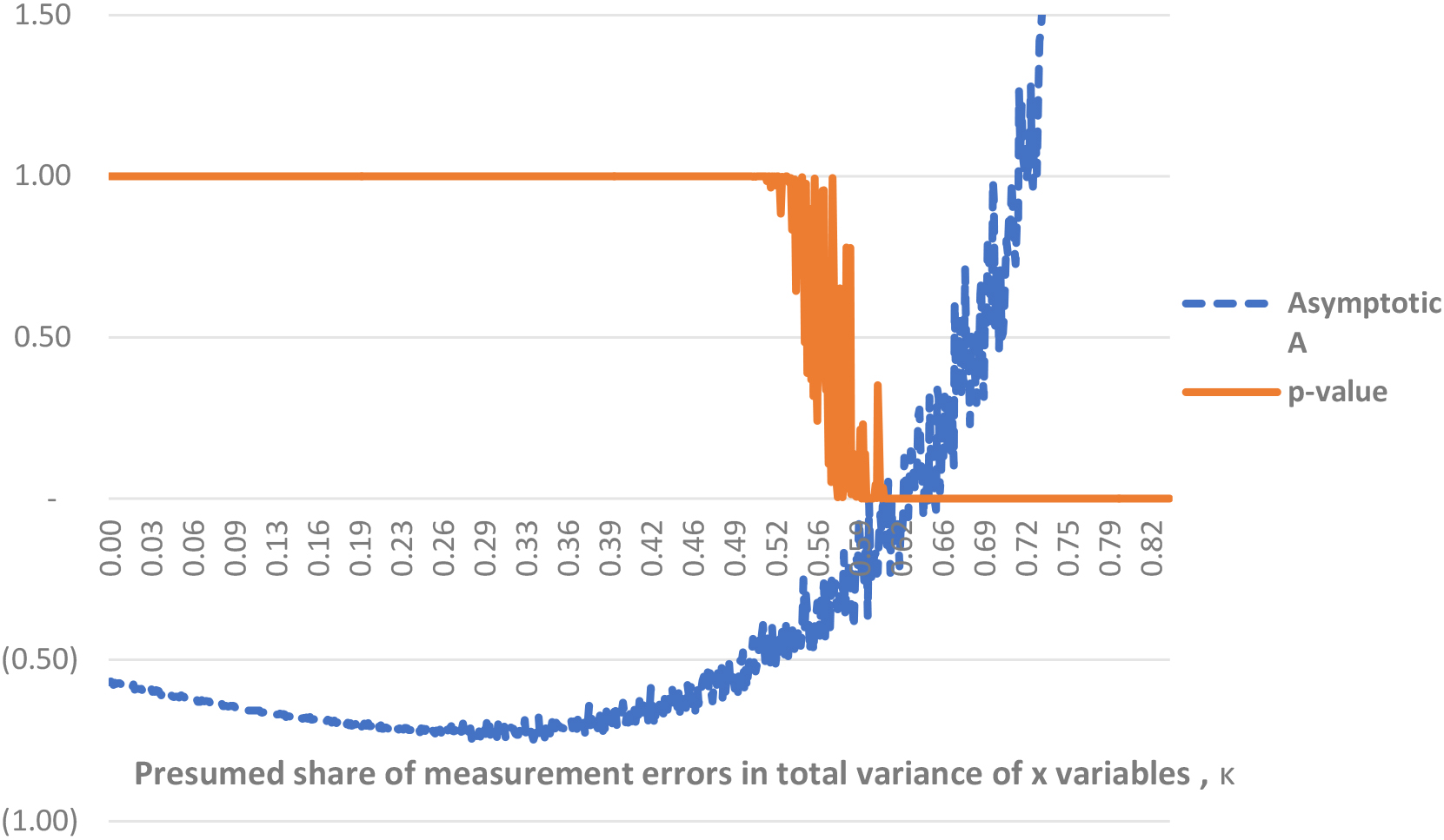
In a practical case, where the covariance matrix of measurement errors in $x$ is unknown, we can use the test with presumed value $S=\kappa\hat{S}_{w},\kappa\in[0,1)$ , as proposed in Appendix 2. Here k is a share of error variance in the total x variance under assumption that relative errors are the same for each x variable. In Fig. 1 we see that for $\kappa\leqslant 0.54$ , the corresponding p-value is close to 1, and for $\kappa\geqslant 0.62$ , the $p$ -value is close to 0. With certain precision, this corresponds to the intervals where the asymptotic value $A_{\infty}$ of the test statistic is negative ( $\kappa<0.62$ ) and positive ( $\kappa>0.62$ ), respectively. See Appendix 2 for the relation between $p$ -values and the behavior of $A_{\infty}$ .

In fact, from all observed in simulations one main idea could be informally derived: the proposed criterion separates situations with and without “improper covariates”. It behaves very differently in those two scenarios. Could we use it for this purpose directly? If one may confidently conclude that a given model with all assumptions about measurement errors contains or not the unobserved covariates, it will be an important result in statistical modeling. This type of criterion could replace many heuristic ones in a large area of research for the “best variables selection” (see, for example, Lipovetsky, 2006, and references therein).

The proposed criterion does not answer this question strictly, but leads to the right direction. It turns out that the key results from (Kukush & Polekha, 2006) combined with ones from the current paper could be used to formulate the correct criterion for answering the question: are there hidden independent covariates in data or not? But this special topic will be considered in a separate paper.

Figure 1.
Asymptotic value of the numerator in (A13) of the test statistic and $p$ -value of the test as a function of $\kappa$ .

In order to demonstrate the effect of the incompleteness of the model, considered above, in more general terms, we performed a separate simulation study. It does not cover all possible sources of the model’s misspecification, but one very common problem: how omitting some variables effects the estimation of the model’s coefficients. It is clear that a researcher is almost never sure that the model is ideally specified, and most often the number of variables used is less than exists in nature. It is a well-known problem, but surprisingly just few simulation studies were performed on it (Erees, 2009), and none, as far as we know, with errors in the variables. Even though we do not file this gap completely, our simple simulation provides some important insight that the bias due to variables omission could be extremely high, that makes the problem of the testing model’s validity very actual. The simulation was organized as follows.

The datasets with 6 independent X and one dependent Y variables by 1000 of observations were set in three versions. First, as random variables slightly correlated among themselves (correlations varied between 0 and 0.55, what is rather typical in the real data; without multicollinearity). Second, the same data set with the error 10%: to each individual value of $x$ the random value from normal distribution with zero mean and 0.1 $x$ standard deviation was added. Third, the same as the second, but with 20% error (0.2 $x$ ). Thus, all X variables were assumed to be measured with the same error rate; it also was true for Y (the error was 0.1y or 0.2y).

Figure 2.
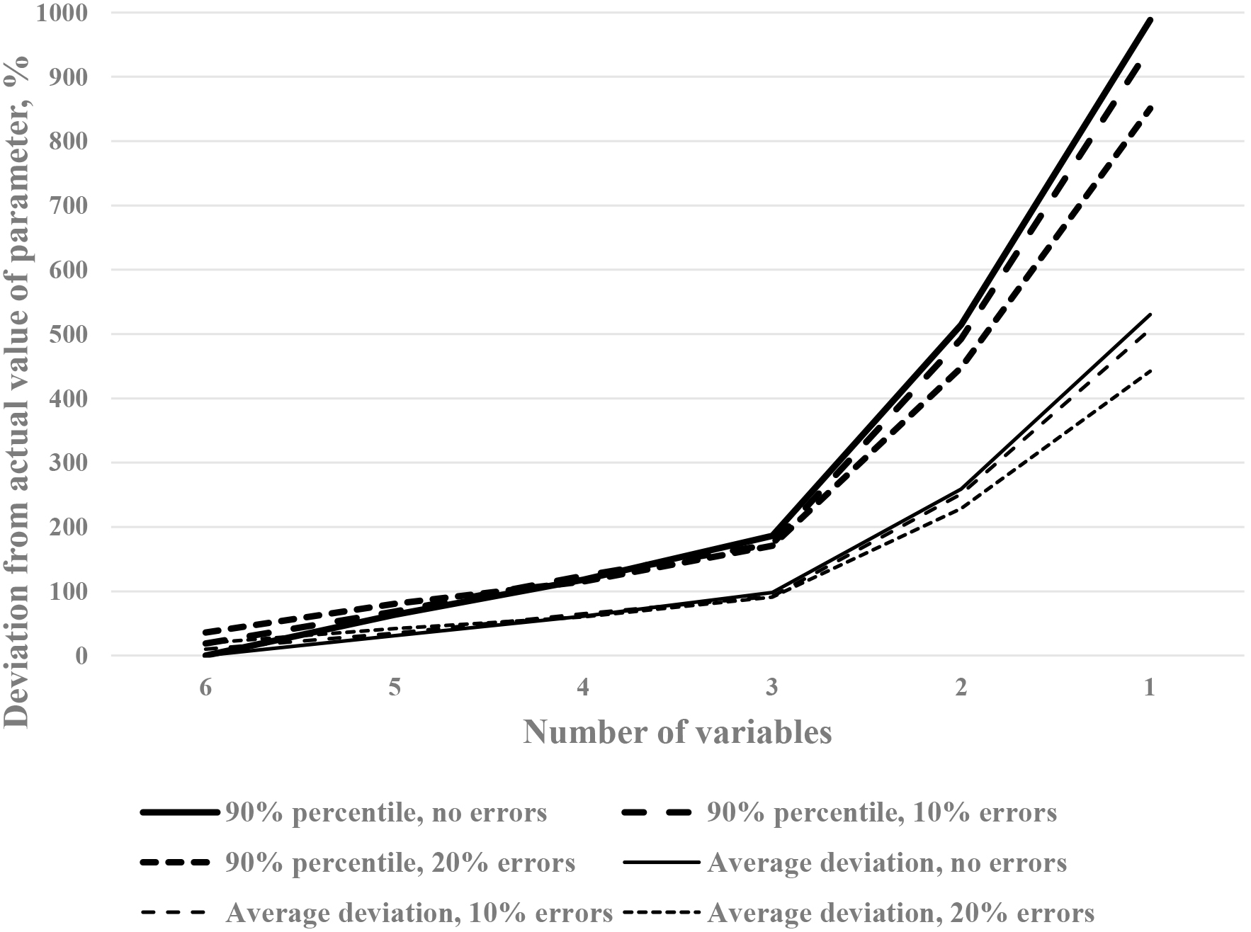
Deviations of the coefficients from the actual values.

Figure 3.
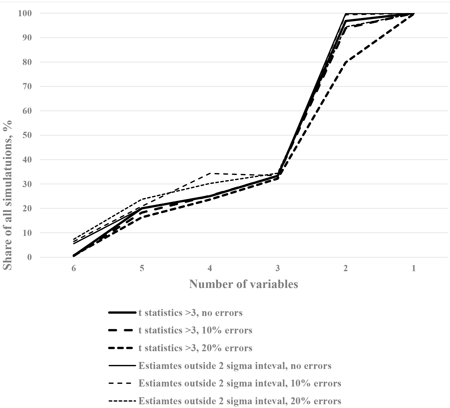
Confidence intervals and t-statistics for deviations from actual values.

Then the sets of one thousand true positive coefficients was created in such a way, that each of them was a random value between 1 and 100 and was used for all three data sets. For example, the first set of the true coefficients (for variables x1, x2, .., x6) was 25, 31, 12, 92, 56, and 45. The second – 85, 13, 28, 47, 91, 89, and 38, and so on thousand times. It means, that no variable was set up as being more important than others during whole simulation. This setting allows for averaging of the results for all variables without loss of generality. The fact that all coefficients were only positive numbers, allows to calculate the deviation* from the real value in percents, as absolute difference between actual and estimated values divided by actual value. It makes all deviations comparable among the different levels and between different variables. Then for each of three datasets, six models were run – from 6 variables of the complete model to 1 variable of the severely incomplete model. The main results of the simulation could be presented in two charts.

Figure 2 shows the behavior of two statistics. The Average deviation is the average value of all deviations for all variables (say, for 5 variables it is an average of 500 values). It is clear that the average deviations of actual values from the estimated are doubled (reach 100%) when the number of variables is 3 instead of 6, after which the deterioration sharply increases and reaches 5-fold difference when just one variable is used.

Another statistic is 90% percentile of the deviations: one may see that ten percent of all deviations exceed nine or ten-fold difference against the actual values when just one variable is in a model (or five-fold with 2 variables).

In Fig. 3 two other indicators are demonstrated. One shows the percent of t-statistics, exceeding 3, i.e., significantly different from the actual values. Again, 3 variables play a role of the threshold here: 30% of all estimates are outside the acceptable bounds for the parameters, while with two variables almost all estimates with or without errors lie in that zone. Similarly, the percentage of estimates outside the borders of the 95% confidence interval (two sigma) more or less repeats the same pattern – a sharp rise after number of variables is less than three.

This simple simulation shows, that the problem of variables’ omission, so common in practice, would often lead to serious deviations of the actual values from the estimates, which cannot be compensated by more sophisticated techniques. Since different studies omit different variables, it may contribute into reproducibility crisis, mentioned earlier.
4. Real data example: Calories in food

Indicators	Inclusion of $x_{3}$ and type of Ho	Sample size
		30	100	500	5000
EIV test, share of rejection	All cases	0.13	0.27	0.41	0.52
	Yes	0.25	0.43	0.52	0.6
	No, Ho true	0.01	0	0	0
	No, Ho false	0	0.21	0.57	0.86
Determination, $R^{2}$	All cases	0.73	0.73	0.73	0.72
	Yes	0.63	0.62	0.63	0.62
	No, Ho true	0.82	0.83	0.82	0.82
	No, Ho false	0.82	0.83	0.82	0.82
Error of type II	All cases	0.60	0.45	0.3	0.19
	Yes	0.71	0.51	0.39	0.30
	0, Ho true	n/a	n/a	n/a	n/a
	0, Ho false	0.99	0.79	0.41	0.14
$p$ -value	All cases	0.47	0.41	0.38	0.37
	Yes	0.34	0.29	0.27	0.26
	No, Ho true	0.89	0.9	0.94	0.97
	No, Ho false	0.33	0.19	0.09	0.02
Correlations with $p$ -values
EIV test	All cases	$-$ 0.47	$-$ 0.61	$-$ 0.77	$-$ 0.91
	Yes	n/a	$-$ 0.69	$-$ 0.79	$-$ 0.93
	No, Ho true	0.00	0.00	0.00	0.00
	No, Ho false	$-$ 0.12	$-$ 0.36	$-$ 0.56	$-$ 0.57
Determination, $R^{2}$	All cases	0.43	0.36	0.30	0.27
	Yes	0.04	0.43	0.37	0.34
	No, Ho true	0.04	0.05	0.14	0.19
	No, Ho false	0.23	0.10	0.03	0.02

	Scaling parameter	Test rejection, %	Determination, R2, %	Error of type II	$p$ -value
Y measurement error, $\sigma$	0.01	26	83	0.37	0.37
	0.05	37	76	0.39	0.42
	0.20	36	59	0.4	0.44
X measurement error, $\delta$	0.01	29	75	0.41	0.38
	0.05	39	74	0.33	0.41
	0.20	31	68	0.41	0.44
Factor f for X3	0.01	20	82	0.77	0.51
	1	31	79	0.61	0.35
	3	84	27	0.05	0.00

To demonstrate how the proposed test may work in practice, let us consider a simple example with real data, which were discussed in (Mandel, 2017, 2018) in connection with casual modeling problem. It is a collection of 872 types of foods, where the content of fats, proteins, carbohydrates, and total amount of calories is measured per 100 grams of food https://www.csun.edu/science/ref/spreadsheets/xls/nutrition.xls. Since calories could be obtained only from those three ingredients (not from, say, water or fiber), the model with three independent covariates is causal, linear and complete. The remaining variance in $y$ (calories), if any, could be explained only by measurement errors in $x$ and $y$ . In that respect, a model is ideal for the study and exactly fits description of the model in Eqs (2) and (3). Let consider application of the proposed test to two situations described earlier: for complete model and for the model with added hidden covariate. We start with the simplest case.

Complete model: no hidden covariates.

A certain number of foods does not have one of the ingredients. We took the subset without fat (241 foods), i.e., just with two independent covariates, Carbs and Proteins (to be called w1 and w2 in Eq. (3)). As expected, the model shows very high goodness-of-fit, with OLS estimates of the coefficients 3.91 and 3.94 and with $R^{2}=$ 95.6%. Those coefficients match perfectly those widely known in the nutrition literature, reported usually just as equal to each other, 4.

Now, let us check the hypothesis about validity of this model. As formulated in Eqs (28)–(35), the test compares two errors in $y$ , measured as variances, the true one and the estimated. We have no idea how big or small the real error in $y$ is, neither how big are the errors in $x$ covariates (which is indeed the case – the publishers of the data did not say anything about errors). In order to test the validity, one has to make plausible assumptions about the errors and make test’s calculations. But what is plausible?

The best way is to use relative errors, i.e., fraction of the presumed ${{\delta}}$ to the standard deviation of the respected covariate $w$ or response variable $y$ . This fraction cannot be higher than 1, and we run the estimates, respectively, in a range from 0 to 1. Another assumption was that relative errors for each covariate are the same (it could be easily relaxed without loss of generality). P/A ratio was also set in a respective range in such a way that its maximum value does not allow the measurement error exceed the standard deviation of $y$ . The results could be briefly summarized as follows.

1.
When critical value of the test in Eq. (30) is set as 3 (which yields the confidence probability $P=$ 0.99), the Ho was not rejected under any conditions.
2.
When critical value was set to 2 ( $P=$ 0.95), the rejection took place only if the assumed measurement errors, both for $x$ and $y$ , are very small.
3.
The rule of thumb recommendation may be provided, that the presumed variance for $y$ measurement error should be about $\textit{RSS}/(n-m)$ , where $n$ is the number of observations and $m$ – the number of covariates. In our case, it gives a relative error close to 90%: the larger presumed values of errors are more preferable than the smaller ones for test to work more confidently. Yet very large values would definitely eliminate any probability of rejection.
4.
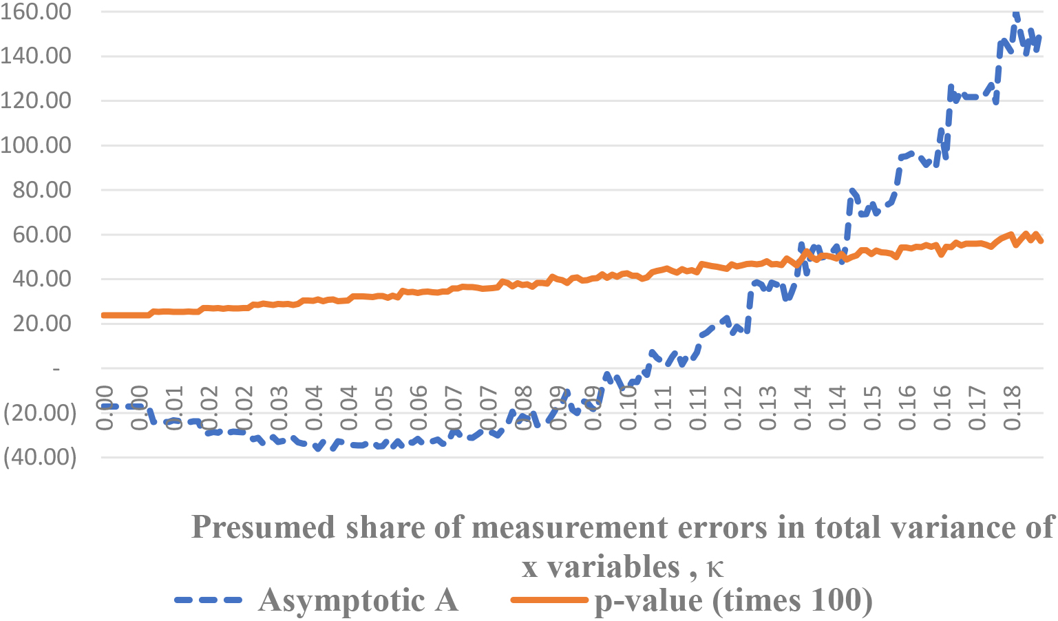
Those conclusions are independently supported by considerations related to the sign of the numerator in Eq. (51). Despite the fact that sample size here is not that big, a chart like one on Fig. 1 shows the similar non-monotone curve for $A_{\infty}$ (Fig. 4). It crosses zero at about 10% point, which corresponds with beginning of $p$ -value raise.
5.
The described effects are intuitively clear, even if not immediately obvious. Imagine, we presume that a data has no measurement errors at all, the function is strictly linear. Of course, Ho should be rejected, because we do observe unexplained variance in $y$ variable! The test demonstrates just that. In this specific dataset, the plausible level of errors in $y$ is very high (see the rule of thumb in the paragraph 3 above), and even for that reason we should not reject hypothesis.

Figure 4.
Asymptotic value of the numerator in (A13) of the test statistic and $p$ -value of the test as a function of $\kappa$ for Carbs and Protein model.

Thus, overall, the MEMV test provides very strong evidence that the model is valid, which is indeed true in this case of the complete model. What if it the model is incomplete?

Misspecified model: hidden covariate.

Let us consider much more common scenario, with hidden covariate(s) in a model, while researcher has no idea about it. For testing we may use the entire food dataset, but use the same two covariates as before assuming that the very notion of Fat is unknown to the statistician. Expectedly, the quality of the regression model drastically dropped, with $R^{2}$ just 15.3% (vs. 95.6% for the complete case discussed earlier), and coefficients severely biased: 2.5 and 5.5 vs correct 4 for both covariates. This model, however, perfectly satisfies the standard statistical requirements: t statistics for coefficients are 10.4 and 8.3, much higher than usually required 3, and $p$ -values are practically zero, thousand times smaller than the infamous 0.05, which once again tells about fragility of all that type of “requirements”. Can the proposed test conclude that something is still wrong?

Yes, it can. The hypothesis that model is correct is rejected immediately and on entire range of assumptions about errors. Difference in presumed errors for $y$ practically is negligible for this conclusion. The test detects, that despite all “perfect” statistics, the model is invalid, and with very high confidence, when $P=$ 0.99 (see more details in Kukush & Mandel, 2019).

But possibly, the test worked very well because the original model was too weak, judging by common sense about low determination (15%), not by other indicators ( $t$ -stat and $p$ -value)? Let us check it on another pair of covariates, giving much more formal “confidence” that model is good. It turned out, that if we exclude Protein, but leave Carb and Fat, the model will seem just perfect: the determination is 95.4%, the coefficients are very close to the real ones – 3.6 and 8.8 (vs. 4 and 9), and, of course, t statistics (63 and 129) and $p$ -values (0) are much smaller than any typically accepted levels. But the model is incomplete, and we know that. What about the test? It does not disappoint even in this difficult for detection situation.

In the same fashion as before, the test rejects the hypotheses, but, remarkably, does it for much shorter range of the available presumed errors for covariates. This range becomes even shorter with increasing of errors for $y$ : up to about 16% for small errors in y and up to 10% when error for $y$ is around 60%. It makes a lot of sense. When determination is very high and the model is valid, big measurement errors in covariates are actually impossible, there is no room for them, and Ho almost never is to be rejected with high confidence on the very narrow range for errors. However, when the same high determination takes place on invalid model, as in this case, the restriction for errors in covariates remains, but its range becomes much larger (by three times) and confidence in rejection much higher (0.99 vs 0.95). Thus, even in this almost extreme case, the test worked and detected the invalidity of the model, which would escape our attention otherwise. The decision is justified with less confidence, in general, than it was in a model with Protein and Carbohydrates, with determination 6 times smaller, but still justified.

Those examples show how the MEMV test could be used in practice. The radical difference between superficially almost identical models shows it very well: in both cases (complete and incomplete) approximation is extremely high ( $R^{2}=$ 0.95), but the test convincingly reveals the qualitative difference. It seems it can play an important role in separation of the complete and incomplete models in the very common situation of errors in variables for any linear models.

Resuming, here are short recommendations how to use the proposed measurement errors model validity test in practice.

1.
If error variance $\sigma_{e}^{2}$ of $y$ variable and error covariance matrix $S_{\delta}$ of $x$ variable are known (like when measurement devises with given calibration are used for both $y$ and $x$ ), use the test directly with $S=S_{\delta}$ and $\sigma_{0}^{2}=\sigma_{e}^{2}$ .
2.
If error variance $\sigma_{e}^{2}$ of $y$ variable is known but error covariance matrix of $x$ variable is unknown, then set $\sigma_{0}^{2}=\sigma_{e}^{2}$ and $S=\kappa\hat{S}_{w},\kappa\in[0,1)$ , where $\hat{S}_{w}$ is a sample covariance matrix of $w$ (see Appendix 2), and use the test for different presumed values $\kappa$ . Plot the dependence of $p$ -value of the test as a function of ${\kappa}$ , i.e., build a chart like the one in Fig. 1. Set the confidence level (e.g., $P=$ 0.99). Indicate the intervals for $\kappa$ where the corresponding $p$ -value is less than $1-P$ (where $H_{0}$ is rejected and the model is invalid), and the intervals where corresponding $p$ -value is greater than or equal to $1-P$ (where $H_{0}$ is not rejected and the model could be valid). Then select one or another interval for $\kappa$ and make the corresponding decision according to your ideas a about possible level of measurement errors of $x$ variable. Since k represents the error’s share in the total x variance, if k is less than presumed level of errors – the Ho is accepted. Keep in mind though, that it is not a universal situation: sometimes a plot for A8 may have several crossing points with the horizontal axis. If you are not able to make the final choice, then you need more information about measurement errors of $x$ variable.
3.
In a the case when the error variance $\sigma_{e}^{2}$ of $y$ variable is known and the error covariance matrix $S_{(1)}$ of some components $x_{(1)}$ of ${x}$ variable is known, while for the rest components $x_{(2)}$ it is unknown, make the analysis similar to the paragraph 2 above with a block diagonal matrix $S$ , with blocks $S_{(1)}$ and $\kappa\hat{S}_{w_{(2)}}$ , $\kappa\in[{0,1})$ , where $\hat{S}_{w_{(2)}}$ is a sample covariance matrix of ${w}_{(2)}$ , a surrogate data for unobservable components $x_{(2)}$ .
4.
If error variance of $y$ variable is unknown and error covariance matrix $S_{\delta}$ of $x$ variables is known, then the proposed test is not applicable. But another test developed in (Kukush & Polekha, 2006) can be used. We intend to study that test in future research.
5.
If error variance of $y$ variable is unknown and error covariance matrix of $x$ variable is unknown or only partially known, one can try the test from (Kukush & Polekha, 2006) with matrix $S$ selected as in the paragraphs 2 or 3 above. This case will be also studied in future research.
6.
Finally, suppose that error variance of $y$ variable $\sigma_{e}^{2}=\lambda\sigma_{\textit{nom}}^{2}$ and error covariance matrix of $x$ variable $S_{\delta}=\lambda S_{\textit{nom}}$ with known characteristics $\sigma_{\textit{nom}}^{2}$ and ${S}_{\textit{nom}}{S}_{\textit{nom}}$ (those nominal values are usually taken from passports of measurement devices) and unknown positive factor $\lambda$ . It may happen, when, for example, all variables are measured with the same device, but accuracy of this device is not precisely known, i.e. we do not know the exact $\lambda$ . Under a presumed upper bound $\lambda_{0}$ , one can check the null hypothesis: “ $\lambda\leqslant\lambda_{0}$ ” (this will be studied in future research); and without a presumed upper bound, one can use a test developed in (Kukush & Tsaregorodtsev, 2017).

5. Conclusion

We considered the classical measurement error Eqs (2) and (3) where the variance-covariance matrix $S$ of the measurement error $\delta$ in the predictors is known (e.g., in situation of repeated observations of covariates or when we trust the passport information about the precision of measurements), and the variance $\sigma^{2}$ of the error in the response is unknown. Given upper estimate of $\sigma^{2}$ , we checked a hypothesis that the true value of $\sigma^{2}$ does not exceed the upper estimate. In case the hypothesis is rejected, we infer that either error in the response variable contains misspecification component (i.e., model lacks explaining covariates), or actual level of measurement errors in the data exceeds the upper estimate. Further study to be performed would demonstrate that this mixture can also be untangled: situation with misspecification could be separated from the one with measurement errors only.

Theoretical exploration, intensive numerical simulations and practical example allow listing the following important features of the proposed MEMV test:

•

under almost all circumstances it separates valid and invalid models with error of type I equal to zero, but with very different level of errors of type II;

•

it is very sensitive to the presence of the hidden (unobservable) covariate and detects it even in situations, when everything tells the opposite: a model seems close to perfect (very high approximation, very good values of traditional indicators, like $p$ -values or t statistics, etc.);

•

sample size $n$ plays generally an expected role in the test – the level of the errors of second type is dramatically decreased when $n$ raises, yet it also demonstrates (not always) the known problem that tendency to reject hypotheses is increasing with rise of the sample size;

•

to make a confident conclusion that only errors determine $y$ variance, while hidden covariates are not presented in the model, one should have many cases available (more than 500 at least);

•

the most important factor among others (like errors in variables, assumptions about the error level, etc.) affecting the correct decision is the relative size of the hidden covariate (i.e., the share of variance of $y$ to be explained by variance in $x$ ): when it is high compared to observed ones, the quality of the decision is dramatically improved (with $p$ -value close to zero), although the test works also when it is not that high;

•

dependence of the correct decision on the assumption about errors in the independent variable is, counter-intuitively, very low, or even close to zero, much smaller than on the same assumptions about errors in covariates;

•

we did not consider the case where $\sigma^{2}$ is unknown and $S=\lambda S_{0}$ with known matrix $S_{0}$ and unknown scalar factor $\lambda$ , because in this case the Eqs (2) and (3) is not identifiable and the regression parameter $c$ cannot be estimated consistently (this is shown in (Cheng & Van Ness, 1999) for the structural normal model, where the errors and regressor $x$ are normally distributed). In future we intend to construct Wald test in the important case, where the variance-covariance matrix of the augmented error $({e,\delta^{T}})^{T}$ is known up to a scalar factor, while some components of the augmented error are allowed to be identical zero.

A survey of more than 1,500 scientists in different fields revealed that more than 80% of the participants consider as the most important improvement to be made to increase the reproducibility of the scientific results is “better understanding statistics” (Amrhein, 2016). Problem of measurement errors, with all its importance and universality, is still out of the mainstream statistical thinking. But without “better understanding” of this problem the lack of reproducibility will embarrass scientific community as it did before and does now. Our study shows a possible way to address some critical topics in one undeservedly neglected area.

Footnotes

Acknowledgments

Authors are grateful to Prof. Y. N. Tyrin for inspirational discussions and suggestions during several last decades.

Appendix 1: Asymptotic properties of estimators

Let us introduce additional conditions on the Eqs (2) and (3) described with two main conditions in Section 2. We start with the moment conditions on error terms.

(iii) For some fixed $\tau>4$ , $E|e|^{\tau}<\infty$ and $E|{|\delta|}|^{\tau}<\infty$ .

Next come conditions on the empirical moments of the regressor. Below $x(i)$ denotes $i$ th coordinate of covariate $x$ . Remember that bar means averaging over $i=1,\ldots,n$ .

(iv) There exists $\lim_{n\to\infty}\overline{xx^{T}}=:\mu_{2}$ , and $\mu_{2}$ is a nonsingular matrix.

(v) There exists $\lim_{n\to\infty}\bar{x}=\mu_{1}$ , and for each $1\leqslant i\leqslant j\leqslant k\leqslant l\leqslant m$ , there exist

$\displaystyle\lim_{n\to\infty}\overline{x(i)x(j)x(k)}=:\mu_{3}({i,j,k}),\lim_{% n\to\infty}\overline{x(i)x(j)x(k)x(l)}=:\mu_{4}({i,j,k,l}).$

(vi) There exists $C>0$ such that for all $n\geqslant 1$ it holds that $\overline{|{|x|}|^{\tau}}\leqslant C$ , where $\tau>4$ comes from condition (iii).

The final condition involves the estimating function $s_{\theta}({y,w;\theta})$ introduced in Eqs (11), (12), and (16). The existence of the limit below will follow from conditions (i–v).

(vii) At the true point of parameter $\theta$ , the matrix

(37) $\displaystyle B:=\lim_{n\to\infty}\frac{1}{n}\mathop{\sum}\limits_{i=1}^{n}Es_% {\theta}({y_{i},w_{i};\theta})s_{\theta}^{T}({y_{i},w_{i};\theta})$

is nonsingular.

Consider also two weaker conditions.

(viii) At the true point of parameter $\theta$ , the matrix

(38) $\displaystyle B_{\sigma^{2}}:=\lim_{n\to\infty}\frac{1}{n}\mathop{\sum}\limits% _{i=1}^{n}Es_{\sigma^{2}}({y_{i},w_{i};\theta})s_{\sigma^{2}}^{T}({y_{i},w_{i}% ;\theta})$

is nonsingular.

(ix) At the true point of parameter $\theta$ , the matrix

(39) $\displaystyle B_{c}:=\lim_{n\to\infty}\frac{1}{n}\mathop{\sum}\limits_{i=1}^{n% }Es_{c}({y_{i},w_{i};\theta})s_{c}^{T}({y_{i},w_{i};\theta})$

is nonsingular.

Below $\to^{d}$ denotes convergence in distribution.

Theorem. For the Eqs (2) and (3), assume conditions (i–vi). Then the next statements hold true.

1. The estimating Eq. (17) has a solution with probability tending to 1 as $n\to\infty$ , and the resulting estimator $\hat{\theta}$ , which is defined in Eqs (15), (8), (14), converges in probability to the true value $\theta$ , moreover

(40) $\displaystyle\sqrt{n}(\hat{\theta}-\theta)\rightarrow^{d}N(0,\Sigma_{\theta}),$

with

(41) $\displaystyle\Sigma_{\theta}=A^{-1}BA^{-1},$ (42) $\displaystyle A=-\lim_{n\to\infty}\frac{1}{n}\mathop{\sum}\limits_{i=1}^{n}E% \frac{\partial s_{\theta}({y_{i},w_{i}})}{\partial\theta^{T}},B=\lim_{n\to% \infty}\frac{1}{n}\mathop{\sum}\limits_{i=1}^{n}Es_{\theta}({y_{i},w_{i}})s_{% \theta}^{T}({y_{i},w_{i}}).$

2. Let $\hat{A}$ be defined in Eq. (24) and

(43) $\displaystyle\hat{B}=\frac{1}{n}\sum_{i=1}^{n}s_{\theta}(y_{1},w_{i};\hat{% \theta})s_{\theta}^{T}(y_{i},w_{i};\hat{\theta}).$

Then $\hat{A}$ and $\hat{B}$ converge in probability to $A$ and $B$ , respectively, and $\hat{\Sigma}_{\theta}=\hat{A}^{+}\hat{B}\hat{A}^{+}$ converges in probability to $\Sigma_{\theta}$ .

3. Under additional condition (viii), asymptotic variance $v_{\sigma^{2}}^{2}$ of $\hat{\sigma}^{2}$ is equal to the lower right entry of $\Sigma_{\theta}$ , and $v_{\sigma^{2}}^{2}>0$ ; under another additional condition (ix), the asymptotic covariance matrix $\Sigma_{c}$ of $\hat{c}$ is positive definite.

4. Under additional condition (vii), the matrix $\Sigma_{\theta}$ is positive definite.

Proof of Statement 1. The symmetric matrix $M_{w}:=\overline{ww^{T}}-S$ converges in probability to the nonsingular matrix $\mu_{2}$ from condition (iv), therefore, $M_{w}$ is nonsingular with probability tending to 1 as $n\to\infty$ . Hence the estimator $\hat{c}$ satisfies Eq. (8) with probability tending to 1 as $n\to\infty$ . From this explicit formula we get directly that $\hat{c}$ is consistent, i.e., it converges in probability to $c$ . Next, the estimator Eq. (10) converges in probability to $\sigma^{2}>0$ , and the right-hand side of Eq. (10) is positive with probability tending to 1 as $n\to\infty$ . Hence the estimator Eq. (14) coincides with Eq. (10) with probability tending to 1 as $n\to\infty$ , and therefore, $\hat{\sigma}^{2}$ is consistent. Thus, the estimating Eq. (17) has a solution with probability tending to 1 as $n\to\infty$ , with components of the estimating function given in Eqs (11) and (12).

The asymptotic normality of $\hat{\theta}$ is proven in a standard way, based on the equality that holds with probability tending to 1:

(44) $\displaystyle S(\hat{\theta})=0,$

where $S(\theta):=\mathop{\sum}\limits_{i=1}^{n}s_{\theta}(y_{i},w_{i};\theta)$ . By Taylor expansion of $S(\hat{\theta})$ in a neighborhood of the true value $\theta$ , we obtain (remember that $\hat{\theta}$ is consistent):

(45) $\displaystyle S(\theta)+\frac{\partial S(\theta)}{\partial\theta^{T}}(\hat{% \theta}-\theta)+r=0,$

with

(46) $\displaystyle|{|r|}|\leqslant O_{P}(1)\cdot||\hat{\theta}-\theta||^{2}=o_{p}(1% )\cdot||\hat{\theta}-\theta||.$

Hereafter $O_{P}(1)$ and $o_{P}(1)$ denote random sequences that are bounded in probability or converge to zero in probability, respectively. Next, by Central Limit Theorem (CLT) in Lyapunov form (see a convenient statement of CLT in Theorem 8 from (Kukush & Tsaregorodtsev, 2016)),

(47) $\displaystyle\frac{1}{\sqrt{n}}S(\theta)\to^{d}N({0,B}),$

and by Law of Large Numbers

(48) $\displaystyle\frac{1}{n}\frac{\partial S(\theta)}{\partial\theta^{T}}\to^{P}A,$

where $\to^{P}$ denotes convergence in probability, matrices $A$ , $B$ are ven in Eq. (42), moreover $A$ is nonsingular due to condition (iv). Now, Eqs (44)–(48) imply that $\sqrt{n}\cdot||\hat{\theta}-\theta||=O_{p}(1)$ , hence $\sqrt{n}\cdot|{|r|}|=o_{P}(1)$ . The convergence Eqs (40)–(42) follows from Eqs (44), (47), (48) and Slutsky’s Lemma (see Theorem 4.1 in (Billingsley, 1999)).

Notice that conditions (i–vi) are used in particular to prove the convergence Eq. (47), to show that the second limit in Eq. (42) exists and to check the corresponding Lyapunov’s condition.

Proof of Statement 2. The convergence in probability of both $\hat{A}$ and $\hat{B}$ follows from the conditions (i–vii) and Law of Large Numbers. This implies the convergence of $\hat{\Sigma}_{\theta}$ because the matrix $A$ is nonsingular and $\hat{A}^{+}\to^{P}A^{-1}$ .

Proof of Statement 3. The matrix $A$ is block-diagonal, and $v_{\sigma^{2}}^{2}=({A_{\sigma^{2}}})^{-2}B_{\sigma^{2}}>0$ under additional condition (viii). Next, under additional condition (ix), $\Sigma_{c}=A_{c}^{-1}B_{c}A_{c}^{-1}$ and it is positive definite.

Proof of Statement 4. Under additional condition (vii), the matrix Eq. (44) is positive definite, because $B$ is positive definite.

This completes the proof of the theorem.

Appendix 2: p -values for large sample size

Consider the Eqs (2) and (3), but now, for simplicity, the vector $x$ is random (and not necessarily centered). Variables $x,e,\delta$ are assumed to be independent, with finite 4th moments. We also assume that conditions (i)–(ii) from Section 2.1 are satisfied, except the following: matrix $S=\textit{Cov}(\delta)$ is now unknown. Denote $S_{w}=\textit{Cov}(w)$ , $S_{x}=\textit{Cov}(x)$ ; we assume that $S_{x}$ is nonsingular. Note that $S_{w}=S_{x}+S$ , and $S_{w}$ is nonsingular as well.

Based on i.i.d. of the observed pairs given in Eq. (6), we want to compute $p$ -value Eq. (2.3). Since $S=\textit{Cov}(\delta)$ is unknown, we use a certain presumed matrix $V_{n}$ instead. Because $S_{w}-S$ is positive definite, the $V_{n}$ will be selected as $V_{n}=\kappa\hat{S}_{w},\kappa\in[0,1)$ where $\hat{S}$ is the sample covariance matrix of $w$ ,

$\displaystyle\hat{S}_{2}=\frac{1}{n-1}\sum_{1}^{n}(w_{i}-\bar{w})(w_{i}-\bar{w% })^{T}.$

Here $\kappa$ regulates the level of the assumed errors in covariates. We also suppose that $\kappa$ is nonrandom, does not depend on the sample size, and has the same values for all x variables. Hence $V_{n}$ converges almost surely (a.s.) to $\kappa S_{w}$ .

Now, we compute the estimator Eq. (7) as

$\displaystyle\hat{c}=({\overline{ww^{T}}-V_{n}})^{+}\overline{wy},$

which converges a.s. to $\Lambda c$ with

(49) $\displaystyle\Lambda=({\textit{Eww}^{T}-\kappa S_{w}})^{-1}({\textit{Exx}^{T}}).$

For the corresponding residual sum of squares RSS (see Section 2.2), the relation holds holds

$\displaystyle\frac{\textit{RSS}}{n}\to^{P1}E({y-({\Lambda c})^{T}w})^{2}=E({c^% {T}({I_{m}-\Lambda^{T}})x+e-({\Lambda c})^{T}\delta})^{2}$ $\displaystyle=c^{T}({I_{m}-\Lambda^{T}})\textit{Exx}^{T}({I_{m}-\Lambda})c+% \sigma^{2}+c^{T}\Lambda^{T}S\Lambda c.$

Hereafter $\to^{P1}$ denotes the almost sure convergence as $n\to\infty$ .

The statistic $T$ from Eq. (2.3) is a fraction; denote its numerator and denominator as $A_{n}$ and $B_{n}^{1/2}/\sqrt{n}$ , respectively. We have

$\displaystyle A_{n}=\frac{\textit{RSS}}{n}-\sigma_{0}^{2}-\hat{c}^{T}V_{n}\hat% {c}\to^{P1}A_{\infty},$ (50) $\displaystyle A_{\infty}:=c^{T}({I_{m}-\Lambda^{T}})\textit{Exx}^{T}({I_{m}-% \Lambda})c+c^{T}\Lambda^{T}({S-\kappa S_{w}})\Lambda c+(\sigma{}^{2}-\sigma_{0% }^{2}),$ $\displaystyle B_{n}\to^{P1}B_{\infty}:=E({y-({\Lambda c})^{T}w})^{4}-({E({y-({% \Lambda c})^{T}w})^{2}})^{2}>0.$

Consequently, we obtain the following asymptotics for $p$ -value Eq. (2.3):

(51) $\displaystyle\text{if }A_{\infty}>0\text{ then }T\to^{P1}+\infty\text{ and }p% \to^{P1}0,$ (52) $\displaystyle\text{if }A_{\infty}<0\text{ then }T\to^{P1}-\infty\text{ and }p% \to^{P1}1,$ (53) $\displaystyle\text{and if }A_{\infty}=0\text{ then }T\to^{P1}O\text{ and }p\to% ^{P1}\frac{1}{2}.$

In cases Eqs (52) and (53), the null hypothesis is not rejected for $n$ large enough (here $\sigma_{0}^{2}$ is quite large), and in case Eq. (51), the null hypothesis Eq. (28) is rejected for $n$ large enough (here $\sigma_{0}^{2}$ is comparatively small). For finite sample, at each interval for $\kappa$ with $A_{\infty}\leqslant 0$ , we have quite large $p$ -values and the null hypothesis is not rejected.

Consider a particular case $c\neq 0$ and $\kappa=0$ (i.e., it is assumed that there is no measurement errors in covariates), then

$\displaystyle\Lambda=\Lambda_{0}:=({\textit{Eww}^{T}})^{-1}({\textit{Exx}^{T}}% ),I_{m}-\Lambda_{0}=({\textit{Eww}^{T}})^{-1}S,$ $\displaystyle A_{\infty}=c^{T}({I_{m}-\Lambda_{0}})^{T}\textit{Exx}^{T}({I_{m}% -\Lambda_{0}})c+c^{T}\Lambda_{0}^{T}S\Lambda_{0}c+(\sigma^{2}-\sigma_{0}^{2}).$

If $\sigma_{0}^{2}<\sigma^{2}$ , then $A_{\infty}>0$ , $H_{0}$ is false and rejected for large $n$ . If

$\displaystyle\sigma_{0}^{2}>\sigma^{2}+c^{T}({I_{m}-\Lambda_{0}})^{T}\textit{% Exx}^{T}({I_{m}-\Lambda_{0}})c+c^{T}\Lambda_{0}^{T}S\Lambda_{0}c,$

then $A_{\infty}<0$ , $H_{0}$ is true and not rejected for large $n$ .

References

Agresti

(2015). Foundations of linear and generalized linear models. John Wiley & Sons.

Amrhein

Greenland

, & McShane

(2019). Scientists rise up against statistical significance. Nature, 567(7748), 305-307.

Baker

(2016). Is there a reproducibility crisis? Nature, 533(7604), 452-454.

Billingsley

(1999). Convergence of probability measures. 2nd ed. John Wiley & Sons, Inc.

Carroll

R.J.

Ruppert

Stefanski

L.A.

, & Crainiceanu

(2006). Measurement error in nonlinear models: a modern perspective. 2nd ed. New York: Chapman and Hall/CRC.

Cheng

C.-L.

, & Van Ness

J.W.

(1999). Statistical regression with measurement error. London: Arnold Publishers.

Demidenko

(2004). Mixed models: theory and applications. John Wiley & Sons.

Demidenko

(2016). The p-value you can’t buy. The American Statistician, 70(1), 33-38.

Erees

(2009). Problem of omitted variable in regression model specification, https://acikerisim.deu.edu.tr/xmlui/bitstream/handle/20.500.12397/8322/243816.pdf?sequence=1#:∼:text=The%20omission%20from%20a%20regression,biased%20estimates%20of%20model%20parameters.

10.

Glymour

Zhang

, & Spirtes

(2019). Review of Causal Discovery Methods Based on Graphical Models.

11.

Gould

, et al. (2023). Same data, different analysts: variation in effect sizes due to analytical decisions in ecology and evolutionary biology. Ecology and Evolutionary Biology, Life Sciences, Research Methods in Life Sciences, https://ecoevorxiv.org/repository/view/6000/.

12.

Janzing

, & Schölkopf

(2018). Detecting non-causal artifacts in multivariate linear regression models. In: Dy, J., & Krause, A., editors. Proceedings of the 35th International Conference on Machine Learning, pp. 2250-2258.

13.

Kukush

(2011). Measurement error models. In: Lovric, M., editor. International Encyclopedia of Statistical Science. Springer, pp. 795-798.

14.

Kukush

, & Polekha

(2006). A goodness of-fit-test for a multivariate errors-in-variables model. Theory of Stochastic Processes, 12(28), no. 3-4, 67-79.

15.

Kukush

, & Tsaregorodtsev

(2016). Goodness-of-fit test in a multivariate errors-in-variables model A⁢X=B. Modern Stochastics: Theory and Applications, 3(4), 287-302.

16.

Kukush

, & Tsaregorodtsev

(2016). Convergence of estimators in the polynomial measurement error model. Theory Probability and Math Statist, 92, 81-91.

17.

Kukush

, & Mandel

(2019). Does Regression Approximate the Influence of the Covariates or Just Measurement Errors? A Model Validity Test. https://arxiv.org/abs/1911.07556.

18.

Lipovetsky

(2006). Entropy criterion in logistic regression and Shapley value of predictors. Journal of Modern Applied Statistical Methods, 5(1), 95-106.

19.

Lipovetsky

(2023a). Review of the book: “Handbook of Measurement Error Models, by G.Y. Yi, A. Delaigle, and P. Gustafson, eds.”. Technometrics, 65(2), 302-304.

20.

Lipovetsky

(2023b). Statistical modeling of implicit functional relations. Stats, 6(3), 889-906.

21.

Mandel

(2017). Troublesome dependency modeling: causality, inference, statistical learning. https://papers.ssrn.com/sol3/papers.cfm?abstract_id=2984045.

22.

Mandel

(2017, 2018). Two-dimensional space in three cultures, Parts 1 and 2. World of Psychology, 4(92), 266-280; 1(93), 229-240.

23.

Mandel

(2018). Causality modeling and statistical generative mechanisms. In: Braverman Readings in Machine Learning. Springer, pp. 148-186.

24.

Morgan

S.L.

, ed. (2014). Handbook of causal analysis in social research. Heidelberg: Springe.

25.

Pearl

(2009). Causality. Cambridge: Cambridge University Press.

26.

Peters

Janzing

, & Schölkopf

(2017). Elements of causal inference: foundations and learning algorithms. Cambridge: The MIT Press.

27.

Schennach

S.M.

(2016). Recent advances in the measurement error literature. Annual Review of Economics, 8(1), 341-377.

28.

Wasserstein

R.L.

, & Lazar

N.A.

(2016). The ASA’s statement on p-values: Context, process, and purpose. The American Statistician, 70(2), 129-133.

29.

G.Y.

Delaigle

, & Gustafson

(eds.) (2021). Handbook of Measurement Error Models. Chapman and Hall/CRC.

A validity test for a multivariate linear measurement error model

Abstract

Keywords

1. Introduction

2.1 Basic regression model

Footnotes

Acknowledgments

Appendix 1: Asymptotic properties of estimators

Appendix 2: p -values for large sample size

References