
Abstract
We obtain new mathematical properties of the exponentiated odd log-logistic family of distributions, and of its special case named the exponentiated odd log-logistic Weibull, and its log transformed. A new location and scale regression model is constructed, and some simulations are carried out to verify the behavior of the maximum likelihood estimators, and of the modified deviance-based residuals. The methodology is applied to the Japanese-Brazilian emigration data.
Introduction
In the survival data analysis literature, it is convenient to consider more flexible distributions to capture a wide variety of symmetric, asymmetric and bimodal behaviors with non-monotonic failure rate function, including as special cases classic distributions, and produce more robust estimates. At present, proposing new distributions to model survival data with non-monotonic failure rate functions is a very important research line in the area of survival analysis. Thus, we initially present new findings for the exponentiated odd log-logistic (EOLL-G) family which can be employed in several applications to real data. Further, we study two new distributions, called the exponentiated odd log-logistic Weibull (EOLLW) and log exponentiated odd log-logistic Weibull (LEOLLW), and construct a location-scale regression based on the last distribution.
Section 2 provides new structural properties of the EOLL-G family. Sections 3 and 4 define the EOLLW and LEOLLW distributions and obtain some of their properties. Section 5 constructs a LEOLLW regression model in location-scale form, reports the maximum likelihood estimates (MLEs), and provides simulations to investigate the accuracy of the estimates. Section 6 define news deviance residuals to assess departures for the propose regression. A real data set is analyzed In Section 7 to show the utility of the new models. Some conclusions are offered in Section 8.
The EOLL-G density
Let
where
Henceforth,
If
where
Some EOLL-G properties were addressed by Alizadeh et al. (2020). We find new ones below.
Some EOLL-G properties follow directly by routine methods in calculus.
Equation (1) gives
In general, depending on the choice of the parent, For the hazard rate function (hrf) of
where
where A straightforward derivative computation leads to
where
with If there is a function
since
Let
where
Let
where
Consider the parent Weibull cdf
Equation (6) yields
The survival function and hrf corresponding to Eq. (6) (for
and
respectively, where
The EOLLW distribution is very flexible due to different forms of its pdf and hrf; see Fig. 1 and Subsections 3.1, 3.2 and 3.3 (for theoretical results).
Plots of the EOLLW 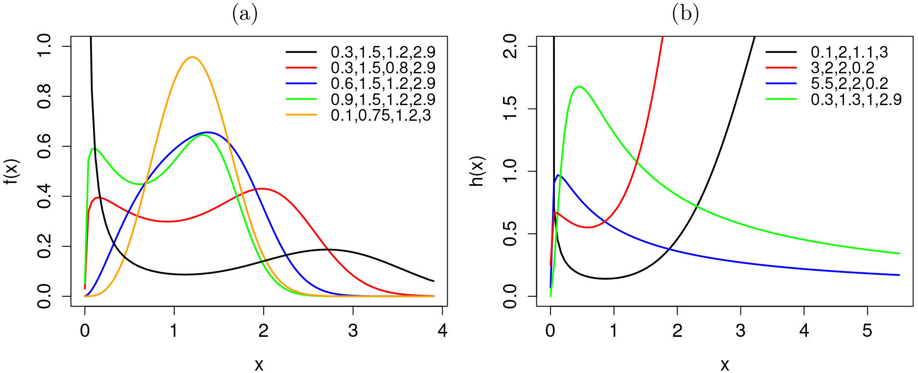
Since
Since
.
If
A critical point of the EOLLW density by property (P4) is a positive root of the nonlinear Eq. (5). A straightforward computation gives
where
The first two derivatives of
and
For
Further,
On the other hand, the first-order derivative de
Setting
where
with
.
Equation (11) has at least one root on
Proof..
Since
The previous proposition guarantees the existence of a critical point of the EOLLW density if
.
If
decreasing or decreasing-increasing-decreasing if unimodal if
Proof..
For
where
Let
On the other hand, let
The proof for the case
It is an arduous task to find (or provide optimal above bounds for the number of) roots of general nonlinear equations. Numerical methods are suitable for this purpose. From the facts that
Plots of Plots of Plots of Plots of
.
If
decreasing or decreasing-increasing-decreasing when decreasing or uni/bimodal or decreasing-increasing-decreasing when
Proof..
Equation (7) gives
By Eq. (7),
.
If
Proof..
Equation (7) gives
.
Notice that, by Theorems 1, 2 and 3, the shape of the EOLLW pdf is independent of the choice of
.
Notice that the shapes of the EOLLW pdf in Fig. 1a are supported by applying Theorem 3.
Let
For simplicity, let
where
where
So, the number of roots of
To state and prove the next result, we define
By choosing
.
Let
If Suppose
If there exists If there does not exist Let
Proof..
For
In what follows, we prove the statement in Item 2. Under the conditions imposed in this one:
The proof of Item 3 follows by using the same steps as in Item 2, so it is omitted. ∎
.
Let
The distribution
The distribution
The distribution
The distribution
In this subsection, we prove that, depending on the choice of parameter
.
The shape parameter
If If
If
Proof..
By Property (P5),
Since
But,
By combining Eqs (21) and (20) with Eq. (19), we obtain that (for any
and that, for
Let
where
The maximum likelihood estimate (MLE)
Under conditions that are fulfilled for parameters in the interior of the parameter space but not on the boundary, the asymptotic distribution of
If
where
Henceforth, let
Plots of the LEOLLW 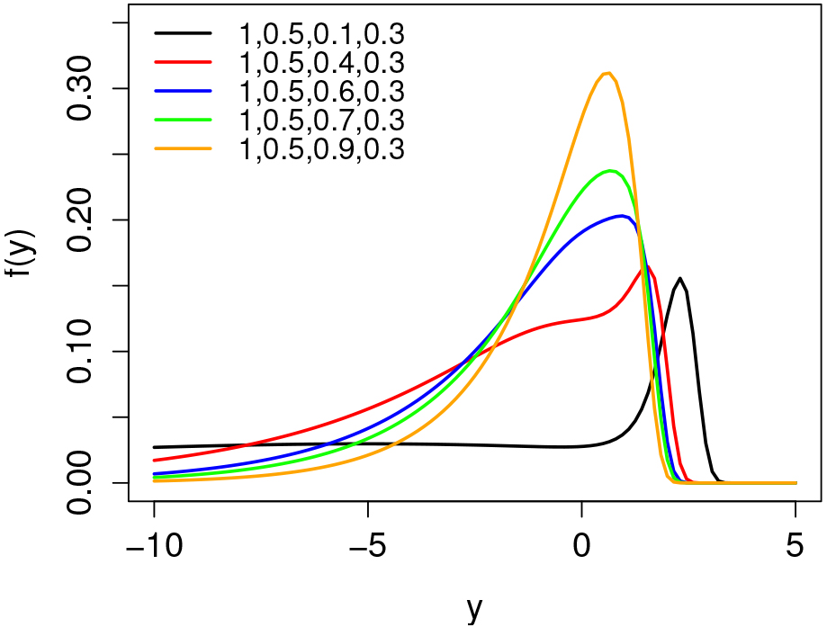
The survival function of
The pdf of
Some properties of
Equation (23) gives
By Property (P5), the stochastic representation for
Let
where
Note that the function
where
First, we define the pdf
where
Second, let
Setting
where
The previous arguments show the following result since
.
The random variable
where
As a consequence of the proposition above, we obtain
The random variable
The random variable
Since
By property (PL3), a critical point of the LEOLLW density satisfies the following equation:
where
and
The following result shows that, regardless of the choice of the parameters, a critical point of the LEOLLW pdf always exists.
.
Equation
Proof..
Since
Since
If If If Further, if
Hence, we have established the following result:
.
If
It is well-known that the standard Gumbel distribution (LEOLLW with
In this subsection, by following Definition 1, we prove that the LEOLLW model has upper light-tail distribution, but the lower tail does not have a well-defined behavior when it is compared with the tail of an exponential distribution. That is, the lower tail of LEOLLW is neither least light-tail nor least heavy-tail.
.
The LEOLLW has upper light-tail distribution and the limit
Here,
Proof..
By Definition 1, to prove that the LEOLLW model has upper light-tail distribution, it must be verified that (for any
Indeed, by Property (P5),
L’Hôpital’s rule gives
But, by considering the change of variables
Since
On the other hand, similarly to the steps done previously, by L’Hôpital’s rule,
where the changing variables
Therefore, we conclude that the limit in Eq. (28) depends on the choice of
The LEOLLW regression model is defined by
Here, the random error
where
Setting
Equation (33) gives the log-odd log-logistic Weibull (LOLLW) regression for
The survival function of
Consider
where
Equation (36) can be maximized using SAS (Proc NLMixed) or R (optim, gamlss) (R Development Core Team, 2022), among others, with initial values for
We perform some simulations in order to evaluate the accuracy of the MLEs. We obtain 1,000 random samples from the LEOLLW
Generate Generate Calculate Generate Calculate the survival times If
Table 1 reports the average estimates (AEs), biases, mean square errors (MSEs) and the empirical coverage probabilities (CPs) for the 95% confidence interval of the MLEs. These results show that the AEs converge to the true parameters and the biases and MSEs decrease when
Update table:
Simulatins results from the fitted LEOLLW regression
The Bias and MSE values correspond to Bias
Residuals are important when determining the adequacy of a regression model and detection of outliers. They play a crucial role in validating the regression by examining the residual plots; see, for example, Cox and Snell (1968), Cook and Weisberg (1982), Collet (2003), Ortega et al. (2008), Silva et al. (2011) and recently Hashimo et al. (2021).
Martingale residuals
We adopt the martingale residuals
Modified deviance residuals
The deviance component residuals (Therneau et al., 1990; Collett, 2003) can be expressed as
where
One thousand samples are generated based on each scenario of
Normal probability plots for 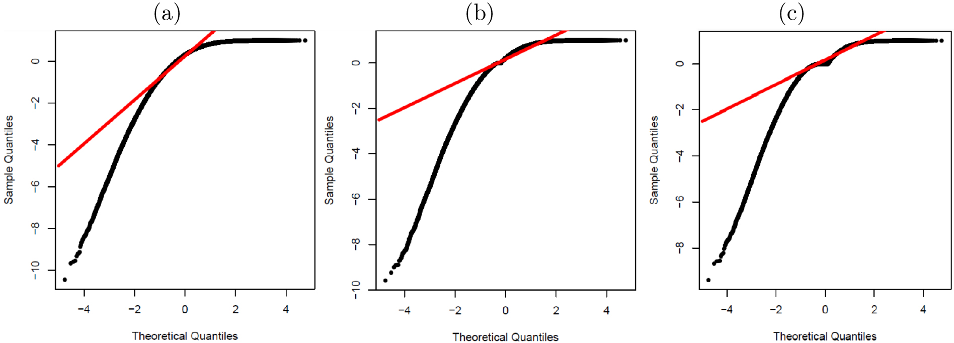
We provide two applications to real data with right censored to demonstrate the usefulness of the EOLLW and LEOLLW distributions.
Application 1: AIDS data
Aids is a pathology that mobilizes the sufferers because of the implications for their interpersonal relationships and reproduction. Therapeutic advances have enabled seropositive women to bear children safely. In this respect, the pediatric immunology outpatient service and social service of the Hospital das Clínicas have a special program for care of newborns of seropositive mothers, to provide orientation and support for antiretroviral therapy to allow these women and their babies to live as normally as possible. We analyze a data set on the time to serum reversal of 143 children exposed to HIV by vertical transmission, born at Hospital das Clínicas (associated with the Ribeirão Preto School of Medicine, in Brazil) from 1995 to 2001, where the mothers were not treated (Silva, 2004). Vertical HIV transmission can occur during gestation in around 35% of cases, during labor and birth itself in some 65% of cases, or during breast feeding, varying from 7% to 22% of cases. Serum reversal or serological reversal can occur in children of HIV-contaminated mothers. It is the process by which HIV antibodies disappear from the blood in an individual who tested positive for HIV infection. As the months pass, the maternal antibodies are eliminated and the child ceases to be HIV positive. The exposed newborns were monitored until definition of their serological condition, after administration of Zidovudin (AZT) in the first 24 hours and for the following 6 weeks.
Table 2 displays the MLEs (and the corresponding standard errors in parentheses) of the model parameters and the values for some models of the following statistics: AIC (Akaike Information Criterion), BIC (Bayesian Information Criterion) and CAIC (Consistent Akaike Information Criterion). The computations were done using the subroutine NLMixed in SAS. These results indicate that the EOLLW model has the lowest AIC, BIC and CAIC values among those values of the fitted models, and therefore it could be chosen as the best model.
MLEs of the model parameters for the the AIDS data, the corresponding SE (given in parentheses) and the measures AIC, BIC and CAIC
MLEs of the model parameters for the the AIDS data, the corresponding SE (given in parentheses) and the measures AIC, BIC and CAIC
Normal probability plots for 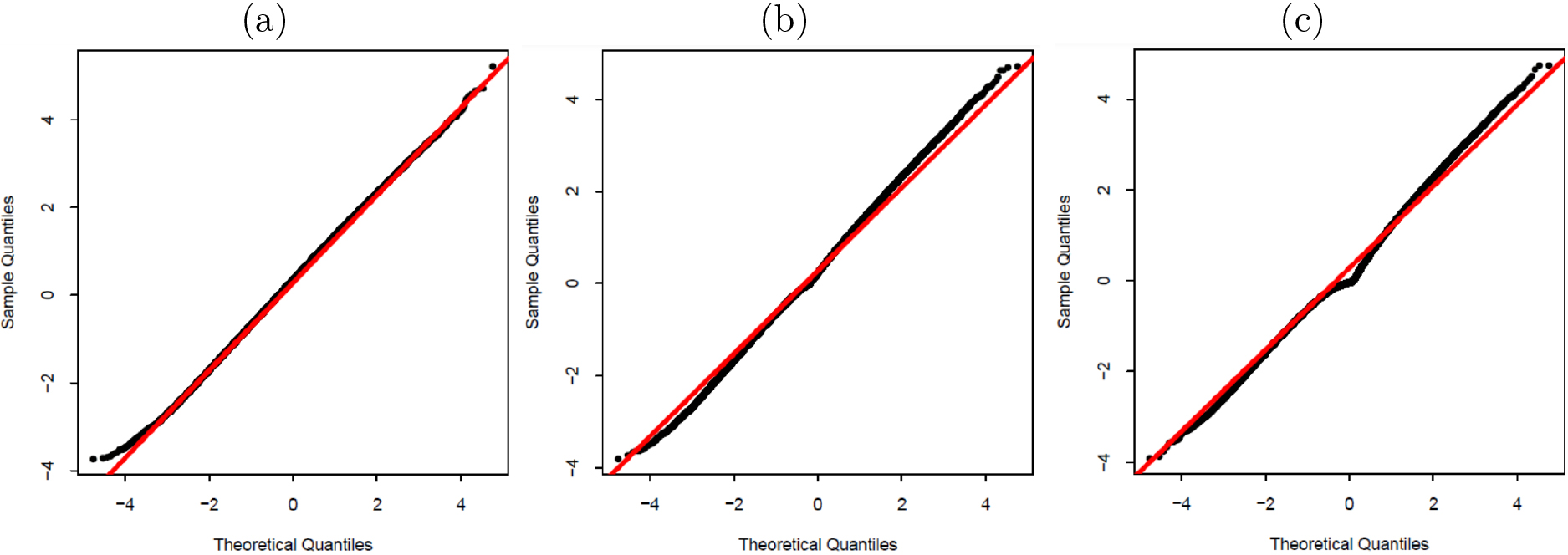
A comparison of the proposed EOLLW model with some of its sub-models via likelihood ration (LR) statistics indicated
The empirical survival function and the estimated survival functions displayed in Fig. 5 support the previous findings.
Kaplan-Meier curves and estimated EOLLW survival functions for AIDS data: (a) EOLLW vs OLLW. (b) EOLLW vs ExpW. (c) EOLLW vs Weibull.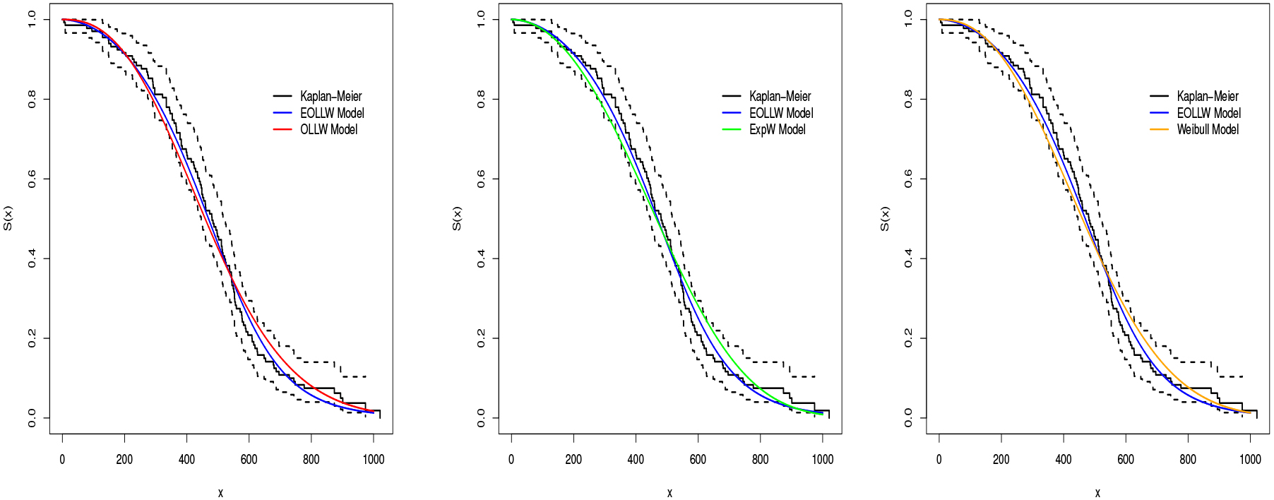
In Fig. 6 we present the graph of the hrf estimated by the EOLLW model. We can observe that the hrf has a unimodal form.
Estimated hrf for the AIDS data.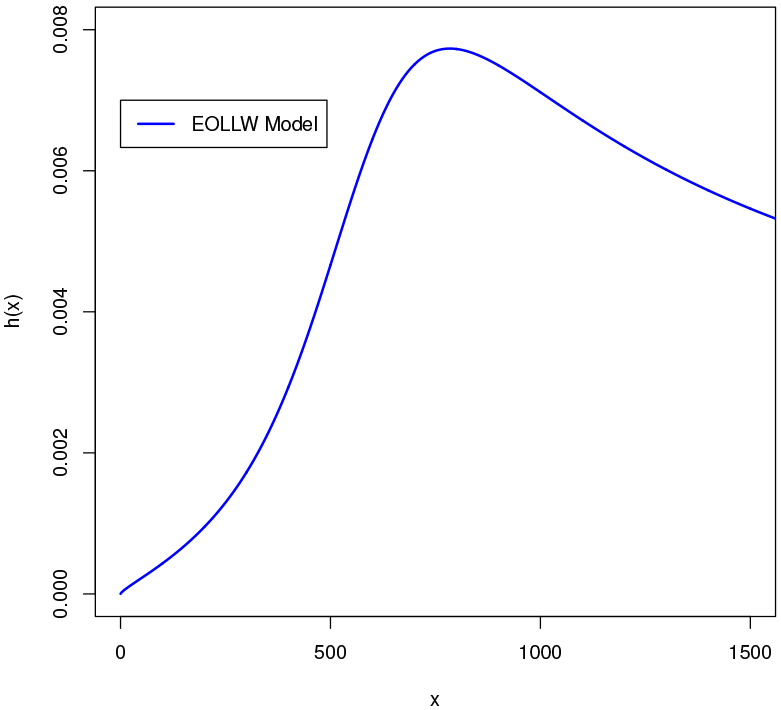
We compare the fits of the LW, LEW, LOLLW and LEOLLW models by calculating the MLEs, their standard errors (SEs) and the values of the Akaike Information Criterion (AIC), Consistent Akaike, Information Criterion (CAIC), and Bayesian Information Criterion (BIC) using the gamlss package in R software (R Core Team, 2022).
Based on technological development and economic growth in the mid-1980s, Japan began to attract many immigrants from Brazil with Japanese ancestry. This phenomenon intensified after June 1990, and at the end of the 1990s these Brazilians formed the third largest community of foreigners living in Japan, with approximately 312,979 people in 2010, behind only Koreans and Chinese (Kawamura, 1999). However, afterward various global crises severely affected Japan, with negative repercussions on the insertion of immigrants in the labor market, leading to the need for professional retraining as a condition for remaining in Japan, unlike the initial situation where high qualification was not required. In response to a request from the Japanese government to the Brazilian government in 2008, Federal University of Mato Grosso (UFMT), by means of the Brazilian Open University program (UAB), together with Tokai University, locted in the city of Hiratsu, Japan, began offering a teacher training course in the distance learning modality. The course, which lasts 4 years, began in 2009, with the aim of qualifying 300 Brazilian teachers working in Japan to work in Brazilian and Japanese schools. Thus, this study seeks to identify the factors that influence the time spent in Japan of the students of the teacher training course offered by UFMT/Tokai, because it is known that the length of stay can be affected by covariables, which are extremely important to the model used in this analysis. The data were obtained by an electronic survey (Babbie, 1999) with the objective to get the characteristics, actions and/or opinions of the group of students using the internet as a learning tool. The survey was conducted in the first school semester of 2010 by means of a reserved site with access only by students, for which 246 completed questionnaires were received. Of these, only 150 were used for analysis because of responses by students of other nationalities. We consider the time (in years) spent in Japan as a response variable counted from the arrival date until July 2012, with censoring of students who returned to Brazil at least once. The variables under study are:
We fit the regression
where the response variable follows the LEOLLW distribution in Eq. (23), and the systematic components are (for
and
The initial values for
The values of AIC, BIC and CAIC are given respectively by: LEOLLW: 172.22, 214.37, 168.26; LOLLW: 293.00, 332.14, 297.06, LExpW: 186.95, 226.08, 191.00 and LW: 216.32, 252.45, 228.39. These values indicate that the LEOLLW regression model can be chosen as the best model. A comparison of the proposed LEOLLW regression model with some of its sub-models via likelihood ration statistics indicated
Table 3 gives the MLEs (and their SEs in parentheses) of the parameters, which reveal that the covariates sex, age, and reasons for migration (study and better living conditions) are significant for the mean parameter
Results from the LEOLLW regression fitted to Japanese-Brazilian emigration data
From the fitted LEOLLW regression to Japan’s data, Fig. 7a gives the plot of the modified deviance residuals Eq. (7) versus the observation index, whereas Fig. 7b gives the normal probability plot with generated envelope (Atkinson, 1987). Both figures support the LEOLLW regression for modelling these data.
(a) Modified deviance residuals versus observation index. (b) Normal probability plot with envelope for the modified deviance residuals.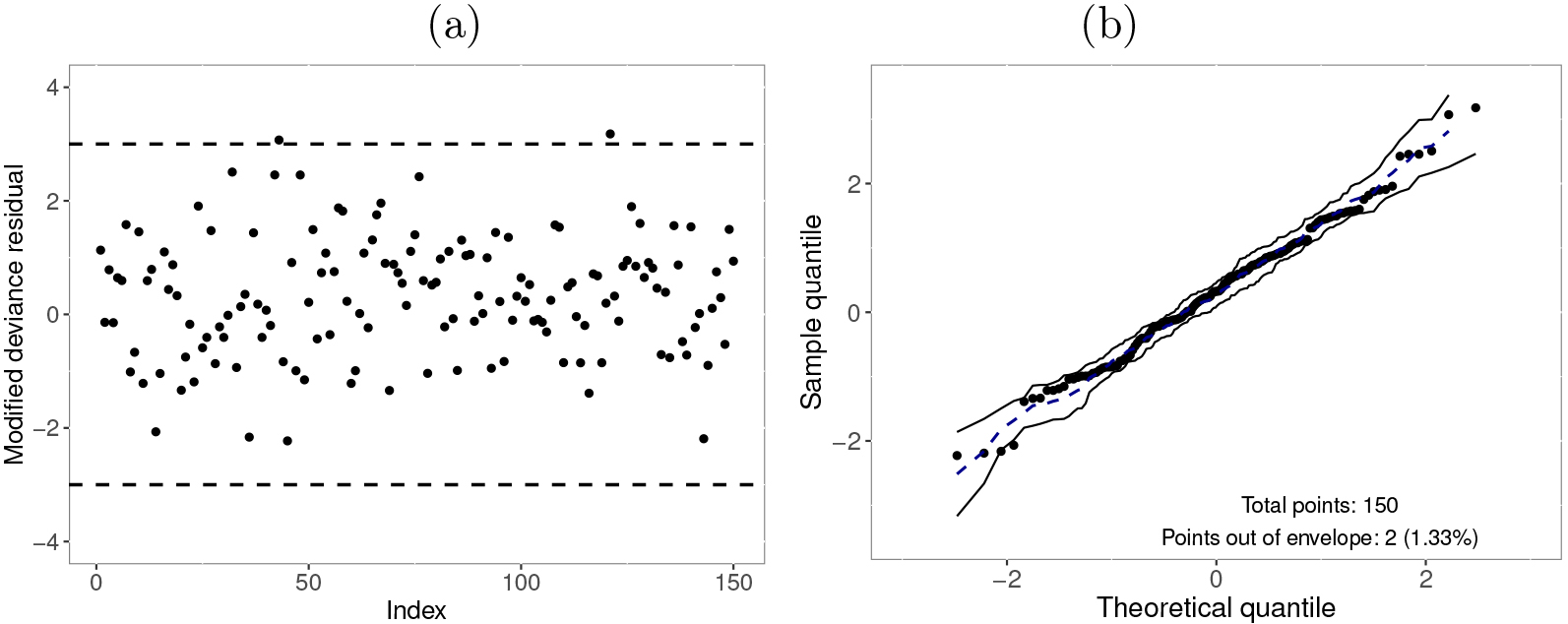
Interpretations for
There is a significant difference between men and women in relation to the length of stay in Japan. The length of stay in Japan tends to decrease when the age increases. A significant difference exists between those who accompanied their family and those seeking better living conditions in relation to the length of stay in Japan. A significant difference exists between those who accompanied their family and those who came for study in relation to the length of stay.
Interpretations for
The variability of the length of stay in Japan tends to decline significantly when the age increases. There is a significant difference between those who accompanied their family and those seeking better living conditions in relation to the variability of the length of stay in Japan. A significant difference exists between those who accompanied their family and those who came for study in relation to the variability of the length of stay in Japan. A significant difference exists between those who accompanied their family and those seeking new experiences in relation to the variability of the length of stay.
We obtained new mathematical properties of the exponentiated odd log-logistic (EOLL-G) family of distributions. Two new distributions, called the exponentiated odd log-logistic Weibull (EOLLW) and log exponentiated odd log-logistic Weibull (LEOLLW), were proposed and their structural properties were studied. We defined a new location-scale regression model based on the LEOLLW distribution for censored data, and calculated the maximum likelihood estimates. Some simulations showed that the empirical distribution of the residuals can be close to the standard normal distribution. We showed that the proposed regression model fitted well to a Japanese-Brazilian emigration data set.
Footnotes
Conflict of interest
On behalf of all authors, the corresponding author states that there is no conflict of interest.