An asymmetric V-shaped distribution

Abstract

This paper proposes a new asymmetric V-shaped distribution for fitting continuous data. In this study, some statistical properties, such as the mean, the median, the variance, the survival, and the hazard function of the new distribution are investigated. Furthermore, we also presented how to generate the proposed asymmetric V-shaped distribution based on two random variables that have uniform distributions. Three examples are presented to illustrate the advantages of the asymmetric V-shaped distribution for some simulated and real-life data sets.

1. Introduction

Data distribution allows us to represent a variable in a compact and simple form. A well-fitting distribution can result in a suitable model for classifying and predicting data, given a data set. Consequently, data distribution modeling has been extensively studied and applied in numerous disciplines, including physic (Afify et al., 2021), economics (Basheer, 2019; Ramos et al., 2019; Vovan et al., 2019), image processing (VoVan & NguyenTrang, 2018), etc.

A distribution can be classified as either unimodal, bimodal, or multimodal (Galtung, 1967). A unimodal distribution is one that has only a single mode. The value of the density function initially rises to its utmost at the mode and then decreases. The normal distribution is the most well-known unimodal distribution. Other examples that can be listed are the Student distribution, the Poisson distribution, the Cauchy distribution, etc. Due to the analytical advantages, most modeling methods are mainly based on some well-known unimodal distributions. Nevertheless, in several practical problems, a single mode does not accurately describe a data set (Braga et al., 2018; Cheng et al., 2017; Ong et al., 2016). Therefore, bimodal distributions need to be studied.

The bimodal distribution is a distribution with two different modes. The larger mode is called major mode and the other mode is called minor mode. The Beta distribution can be either a unimodal or a bimodal distribution, depending on its shape parameters (Jeffreys, 1946; Mazucheli & Menezes, 2019). The Gaussian mixture distribution, which was first proposed by Karl Pearson, is another multimodal distribution (Heggeseth et al., 2018; Rahmani et al., 2020). This is a compound distribution composed of $k$ Gaussian distributions. When $k=$ 2, the Gaussian mixture distribution becomes a bimodal distribution. In addition to the Gaussian mixture distribution, several compound distributions proposed in the literature can be considered as a multimodal distribution (Ahmad et al., 2022; Chesneau et al., 2019; Moreau, 2021; Para et al., 2020; Punzo et al., 2018; Vasconcelos et al., 2020). Some less familiar bimodal distributions are the U-shaped and the V-shaped distributions. In a U-shaped distribution, the probability density function value is greatest at the extremes of data and fast decreases to a minimum in the middle of the distribution. Similarly, the V-shaped probability density distribution value is high at the two ends of the data and decreases towards the middle part.

To our knowledge, V-shaped distribution was rarely studied in literature and was only presented for symmetric data (Mauris, 2009; Rinne, 2014). However, there is evidence of an asymmetric V-shaped distribution in some problems. For example, in the financial market, the probability that a trader takes his/her profit increases as the magnitude of the profit increases. Additionally, the positive side has a steeper slope than the negative side (An, 2016; Ben-David & Hirshleifer, 2012). This phenomenon produces an asymmetric V-shaped distribution for the obtained profit. As a result, this paper proposes a new asymmetric V-shaped distribution. Because “asymmetric” is a more general concept compared to “symmetric”, the proposed distribution is expected to have a higher level of generality. Thus, it can be a more flexible and suitable distribution compared to the existing symmetric V-shaped distributions. Besides, this distribution provides a new method for researchers in various fields to model a data set. Based on the proposed probability density function, we further present the cumulative distribution function, and other statistical properties, such as mean, median, variance, survival function and Hazard function.

The rest of the paper is presented as follows. Some related bimodal distributions are presented in Section 2. Section 3 presents the new asymmetric V-shaped probability density and cumulative distribution functions. Statistical parameters such as mean, median, variance, survival function, and hazard function, are also presented in this section. The numerical examples are presented in Section 4 and the conclusion is provided in Section 5.

2. Related works

2.1 Beta distribution

Suppose that $x$ is a random variable on the interval $[0,1]$ and has the Beta distribution, $(\mathrm{Beta}(\alpha ,\beta ))$ . The probability density function of $x$ is defined as Eq. (1).

$f(x)={\displaystyle \frac{\mathrm{\Gamma }(\alpha +\beta )}{\mathrm{\Gamma }(\alpha )\mathrm{\Gamma }(\beta )}}{x}^{\alpha -1}{(1-x)}^{\beta -1}\hspace{1em}\text{for}\hspace{1em}0⩽x⩽1,$(1)

where $\mathrm{\Gamma }(\alpha )=\underset{0}{\overset{\mathrm{\infty }}{\int }}{x}^{\alpha -1}{e}^{-x}\mathrm{d}x$ .

The standard Beta distribution can be extended to the interval $[a,b]$ using the generalized Beta distribution $\mathrm{beta}(\alpha ,\beta ,a,b)$ where $a$ and $b$ stand for the minimum and the maximum values of $x$ . Also, it can be noted that the Beta is a flexible distribution. For example, $\mathrm{beta}(0,0)$ approaches a Bernoulli distribution, $\mathrm{beta}(1,1)$ approaches a Uniform distribution whereas $\mathrm{beta}(1/2,1/2)$ approaches a bimodal U-shaped distribution. Nevertheless, no report indicated the parameters by which the Beta distribution can approach a V-shaped distribution.

2.2 Gaussian mixture distribution

A Gaussian mixture distribution can represent a bimodal distribution using Eq. (2).

$f(x)=w_{1}N(x|{\mu }_1,{\sigma }_1^2)+w_{2}N(x|{\mu }_2,{\sigma }_2^2),$(2)

where $N(x|{\mu }_i,{\sigma }_i^2)$ is the probability density function of the $i$ -th normal distribution, $w_i$ is the $i$ -th mixing parameter, and $w_1+w_2=1$ . Suppose that $p_i$ is indicative of $N({\mu }_i,{\sigma }_i^2)$ , and $w=w_1$ . We have the following Eq. (3), which is a simplified equation to represent a bimodal distribution.

$f(x)=w{p}_1(x)+(1-w)p_2(x).$(3)

2.3 Arcsine distribution

A random variable $X$ on the interval $[a,b]$ has the arcsine distribution $\mathrm{Arcsine}(a,b)$ , or U-shaped distribution if its probability density function is given by:

$f(x)={\displaystyle \frac{1}{\pi \sqrt{(x-a)(b-x)}}}.$(4)

2.4 Symmetric V-shaped distribution

The probability density function of a symmetric V-shaped distribution is given by

$f(x)=\{\begin{array}{ccc}{\displaystyle \frac{2(2a+b-2x)}{b^2}}\hfill & \mathrm{for}\hfill & a⩽x<a+{\displaystyle \frac{b}{2}},\hfill \\ {\displaystyle \frac{2(2x-2a-b)}{b^2}}\hfill & \mathrm{for}\hfill & a+{\displaystyle \frac{b}{2}}⩽x<a+b,\hfill \end{array}$(5)

where $X$ is a random variable on the interval $[a,a+b]$ . It can be seen from Eq. (5) that $f(x)$ always decreases from $a$ to the range’s middle point $a+b/2$ and increases after that. As a result, it always produces a symmetric but not an asymmetric distribution.

3. The proposed asymmetric V-shaped distribution

3.1 Probability density function and cumulative distribution function

A random variable $X$ on the interval $[a,b]$ has an asymmetric V-shaped distribution, $X\sim \mathrm{aV}(a,m,b)$ , if its probability density function is given by Eq. (6):

$f(x)=\{\begin{array}{ccc}\hfill {\displaystyle \frac{2}{b-a}}{\displaystyle \frac{m-x}{m-a}}\hfill & \hfill \mathrm{for}\hfill & \hfill a⩽x<m,\hfill \\ \hfill {\displaystyle \frac{2}{b-a}}{\displaystyle \frac{x-m}{b-m}}\hfill & \hfill \mathrm{for}\hfill & \hfill m⩽x⩽b,\hfill \\ \hfill 0\hfill & \hfill \mathrm{otherwise}\hfill & \end{array}$(6)

where $m$ gets an arbitrary value in the range $[a,b]$ . It can be seen from Eq. (6) that $f(x)$ linearly decreases from $a$ to $m$ and then linearly increases. Because $m$ is not always the midpoint but it could be any value in the range $[a,b]$ , $f(x)$ is not always a symmetric but it could be an asymmetric function. Therefore, the proposed probability density function in Eq. (6) has a higher generality compared to Eq. (5).

Figure 1.

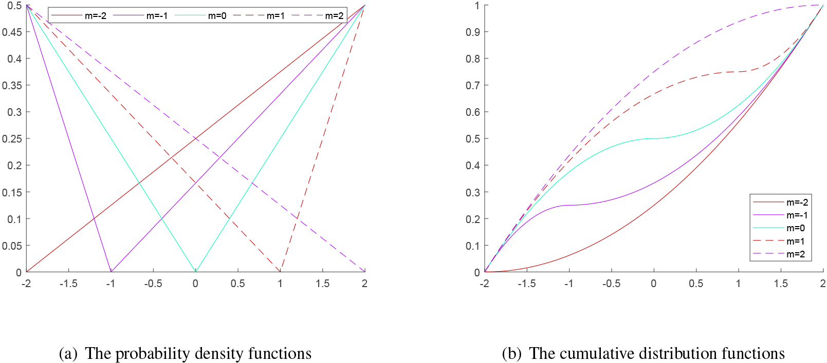
The probability density functions and the cumulative distribution functions of asymmetric V-shaped distribution for various values of $m$ .

It can be easily shown that $f(x)⩾0,\forall x$ and $\int f(x)dx=1$ . Also, by integrating $f(x)$ , the cumulative distribution function $F(x)$ can be shown as:

$F(x)=\{\begin{array}{ccc}{\displaystyle \frac{m-a}{b-a}}-{\displaystyle \frac{{(m-x)}^2}{(b-a)(m-a)}}\hfill & \mathrm{for}\hfill & a⩽x<m\hfill \\ {\displaystyle \frac{m-a}{b-a}}+{\displaystyle \frac{{(x-m)}^2}{(b-a)(b-m)}}\hfill & \mathrm{for}\hfill & m⩽x⩽b\hfill \end{array}$(7)

The probability density functions and the cumulative distribution functions for $a=-2$ , $b=2$ , and various values of $m$ are shown in Fig. 1a and b. It can be seen from Fig. 1 that the proposed distribution is quite flexible due to the parameter $m$ . For example, when $m\ne 0=(a+b)/2$ , the density function is asymmetric; when $m=0=(a+b)/2$ , the density function becomes symmetric; when $m=a=-2$ or $m=b=2$ , the density function is simplified to be a linear function ascending/descending from $a$ to $b$ .

3.2 Statistical properties of the proposed asymmetric V-shaped distribution

.

Let $X$ have an asymmetric V-shaped distribution, $X\sim \mathrm{aV}(a,m,b)$ , $\mathrm{E}(X)$ , $\mathrm{Med}(X)$ and $\mathrm{Var}(X)$ stand for the population mean, median and variance. We have the following statistical properties:

$1.\mu =\mathrm{E}(X)={\displaystyle \frac{2b+2a-m}{3}}.$(8) $2.\mathrm{Med}(X)=\{\begin{array}{ccc}{\displaystyle \frac{b+(\sqrt{2}-1)m}{\sqrt{2}}}\hfill & \mathrm{for}\hfill & m<{\displaystyle \frac{a+b}{2}}.\hfill \\ m-\sqrt{(m-a)(m-{\displaystyle \frac{a+b}{2}})}\hfill & \mathrm{for}\hfill & m⩾{\displaystyle \frac{a+b}{2}}.\hfill \end{array}$(9) $3.\mathrm{Var}(X)={\displaystyle \frac{1}{18}}(b^2+a^2-7ab)-{\displaystyle \frac{5}{18}}m(m-a-b).$(10)

Proof..

1. We have,

${\displaystyle {\int }_a^m}xf(x)dx={\displaystyle {\int }_a^m}{\displaystyle \frac{2}{(b-a)(m-a)}}(mx-x^2)dx={\displaystyle \frac{2}{(b-a)(m-a)}}\left({\displaystyle \frac{m^3}{2}}-{\displaystyle \frac{m^3}{3}}-{\displaystyle \frac{m{a}^2}{2}}+{\displaystyle \frac{a^3}{3}}\right)={\displaystyle \frac{2}{(b-a)}}\left({\displaystyle \frac{m^2}{2}}(m+a)-{\displaystyle \frac{1}{3}}(m^2+am+a^2)\right).$(11)

and

${\displaystyle {\int }_m^b}xf(x)dx={\displaystyle {\int }_m^b}{\displaystyle \frac{2}{(b-a)(b-m)}}(x^2-mx)dx={\displaystyle \frac{2}{(b-a)(b-m)}}\left({\displaystyle \frac{b^3}{3}}-{\displaystyle \frac{m{b}^2}{2}}-{\displaystyle \frac{m^3}{3}}+{\displaystyle \frac{m^3}{2}}\right)={\displaystyle \frac{2}{(b-a)}}\left({\displaystyle \frac{1}{3}}(b^2+bm+m^2)-{\displaystyle \frac{m^2}{2}}(m+b)\right).$(12)

Get sum of Eqs (11) and (12), and then simplify it, we obtain Eq. (8).

2. Let $x_{\mathrm{med}}=\mathrm{Med}(X)$ is the median of $X$ .

For $m<\frac{a+b}{2}$ , assuming that $x_{\mathrm{med}}<m$ , using the definition of Median, we have:

${\displaystyle \frac{{(m-a)}^2-{(m-x_{\mathrm{med}})}^2}{(b-a)(m-a)}}={\displaystyle \frac{1}{2}}\iff {(m-x_{\mathrm{med}})}^2={(m-a)}^2-{\displaystyle \frac{1}{2}}(b-a)(m-a)=(m-a)\left(m-{\displaystyle \frac{a+b}{2}}\right)<0.$

The above inequality shows that the assumption of $x_{\mathrm{med}}<m$ is untrue.

Now, assuming that $x_{\mathrm{med}}⩾m$ , using the definition of Median, we have:

${\displaystyle \frac{(m-a)(b-m)+{(x_{\mathrm{med}}-m)}^2}{(b-a)(b-m)}}={\displaystyle \frac{1}{2}}\iff {(m-x_{\mathrm{med}})}^2={\displaystyle \frac{{(b-m)}^2}{2}}.$

Because $m⩽x_{\mathrm{med}}<b$ , the above equality is equivalent to $x_{\mathrm{med}}-m=\frac{b-m}{\sqrt{2}}$ . or

$x_{\mathrm{med}}={\displaystyle \frac{b+(\sqrt{2}-1)m}{\sqrt{2}}}.$(13)

For $m⩾\frac{a+b}{2}$ , it can be easily proved that the assumption of $x_{\mathrm{med}}⩾m$ is untrue.

Now, let $x_{\mathrm{med}}<m$ , using the definition of Median, we have:

${(m-x_{\mathrm{med}})}^2=(m-a)\left(m-{\displaystyle \frac{a+b}{2}}\right).$

Because $m⩾x_{\mathrm{med}}>(a+b)/2$ , the above equality is equivalent to

$x_{\mathrm{med}}=m-\sqrt{(m-a)\left(m-{\displaystyle \frac{a+b}{2}}\right)}.$(14)

Based on Eqs (13) and (14), we have Eq. (9).

3. We have

${\displaystyle {\int }_a^m}{x}^{2}f(x)dx={\displaystyle {\int }_a^m}{\displaystyle \frac{2}{(b-a)(m-a)}}(m{x}^2-x^3)dx={\displaystyle \frac{2}{(b-a)(m-a)}}\left({\displaystyle \frac{m^4}{3}}-{\displaystyle \frac{m^4}{4}}-{\displaystyle \frac{m{a}^3}{3}}+{\displaystyle \frac{a^4}{4}}\right)={\displaystyle \frac{1}{6}}{\displaystyle \frac{m^3+m^{2}a+m{a}^2-3a^3}{b-a}}.$(15)

and

${\displaystyle {\int }_m^b}{x}^{2}f(x)dx={\displaystyle {\int }_m^b}{\displaystyle \frac{2}{(b-a)(b-m)}}(x^3-m{x}^2)dx={\displaystyle \frac{2}{(b-a)(b-m)}}\left({\displaystyle \frac{b^4}{4}}-{\displaystyle \frac{m{b}^3}{3}}-{\displaystyle \frac{m^4}{4}}+{\displaystyle \frac{m^4}{3}}\right)={\displaystyle \frac{1}{6}}{\displaystyle \frac{3b^3-m{b}^2-b{m}^2-m^3}{b-a}}.$(16)

Get sum of Eqs (15) and (16), and then simplify it, we obtain

$\mathrm{E}(X^2)={\displaystyle \frac{1}{2}}(a^2+ab+b^2)-{\displaystyle \frac{1}{6}}(m^2+ma+mb).$(17)

Then

$\mathrm{Var}(X)=\mathrm{E}(X^2)-\mathrm{E}{(X)}^2={\displaystyle \frac{1}{2}}(a^2+ab+b^2)-{\displaystyle \frac{1}{6}}(m^2+ma+mb)-{\displaystyle \frac{1}{9}}{(2b+2a-m)}^2.$

Simplify the above equation we obtain Eq. (10). ∎

.

If $X$ has a symmetric V-shaped distribution on $[a,b]$ , then $\mathrm{E}(X)=\mathrm{Med}(X)=m$ and $\mathrm{Var}(X)=\frac{m^2-ab}{2}$ .

Proof..

Using $m=\frac{a+b}{2}$ and Theorem 3.1, we get Theorem 3.2. ∎

.

If $X,Y$ have Uniform distributions on $[0,1]$ , $X,Y\sim \mathrm{U}(0,1)$ , then the random variable $Z=\mathrm{sgn}(X-Y)\max \{X,Y\}$ has a V-shaped distribution, $Z\sim \mathrm{aV}(-1,0,1)$ .

Proof..

Because $Y\sim \mathrm{U}(0,1)$ , $-Y\sim \mathrm{U}(-1,0)$ . Let $Z_1=X-Y$ , we have:

$f_{Z_1}(z_1)={\displaystyle {\int }_{-\mathrm{\infty }}^{\mathrm{\infty }}}{f}_X(x)f_{-Y}(z_1-x)dx={\displaystyle {\int }_0^1}{f}_{-Y}(z_1-x)dx.$

Because $-Y\sim \mathrm{U}(-1,0)$ , $f_{-Y}(z_1-x)=1$ if $-1⩽z_1-x⩽0$ or $z\in [-1,1]$ ; for other cases $f_{-Y}(z_1-x)=0$ .

Now, for $-1⩽z_1⩽0$

$f_{Z_1}(z_1)={\displaystyle {\int }_0^{z_1+1}}dx=1+z_1,$

and for $0<z_1⩽1$

$f_{Z_1}(z_1)={\displaystyle {\int }_{z_1}^1}dx=1-z_1.$

Therefore,

$f_{Z_1}(z_1)=\{\begin{array}{ccc}\hfill 1+z_1\hfill & \hfill \mathrm{for}\hfill & \hfill -1⩽z_1⩽0\hfill \\ \hfill 1-z_1\hfill & \hfill \mathrm{for}\hfill & \hfill 0<z_1⩽1\hfill \\ \hfill 0\hfill & \hfill \mathrm{otherwise}\hfill & \end{array}$(18)

It can be implied from Eq. (18) that $Z_1$ has the triangular distribution and $P(Z_1<0)=P(Z_1>0)=1/2$ . Hence, the variable $Z_2=\mathrm{sgn}(X-Y)=\mathrm{sgn}(Z_1)$ has the Bernoulli distribution with $p=1/2$ .

Now, let $Z_3=\max \{X,Y\}$ , we have $f(z_3)=2z_3$ . We also have, $Z=\mathrm{sgn}(X-Y)\max \{X,Y\}=Z_2{Z}_3$ . Therefore,

$F(z)=P(Z_2{Z}_3⩽z)=P(Z_2{Z}_3⩽z|Z_2=-1)P(Z_2=-1)+P(Z_2{Z}_3⩽z|Z_2=1)P(Z_2=1)={\displaystyle \frac{1}{2}}P(Z_3⩾-z)+{\displaystyle \frac{1}{2}}P(Z_3⩽z).$(19)

For $z<0$ , Eq. (19) becomes:

$F(z)={\displaystyle \frac{1}{2}}P(Z_3⩾-z)={\displaystyle {\int }_{-z}^1}2z_3\mathrm{d}{z}_3={\displaystyle \frac{1-z^2}{2}}.$(20)

For $z⩾0$ , Eq. (19) becomes:

$F(z)={\displaystyle \frac{1}{2}}+{\displaystyle \frac{1}{2}}P(Z_3⩽z)={\displaystyle \frac{1}{2}}+{\displaystyle {\int }_0^z}2z_3\mathrm{d}{z}_3={\displaystyle \frac{1}{2}}+{\displaystyle \frac{z^2}{2}}.$(21)

It can be seen from Eqs (20) and (21) that $F(z)$ is the cumulative distribution function of an asymmetric V-shaped distribution with $a=-1,m=0,b=1$ .

∎

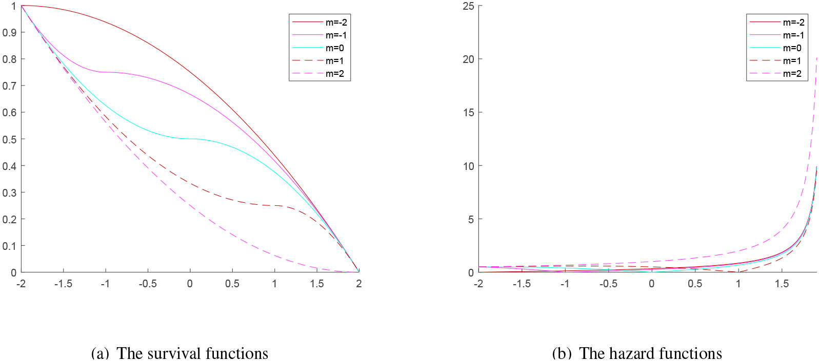
3.3 Survival function and hazard function

The survival function describes the probability that an individual will not fail after a certain time. The hazard function or the failure rate function represents the probability that an individual will fail in a period of time. Mathematically, the survival function is given by $S(x)=1-F(x)$ and the hazard function is given by $h(x)=\frac{f(x)}{S(x)}$ . Figure 2 illustrates the survival and hazard functions for various choices of asymmetric V-shaped distribution.

Figure 2.

The survival and hazard functions of asymmetric V-shaped distribution for various values of $m$ .

Figure 3.

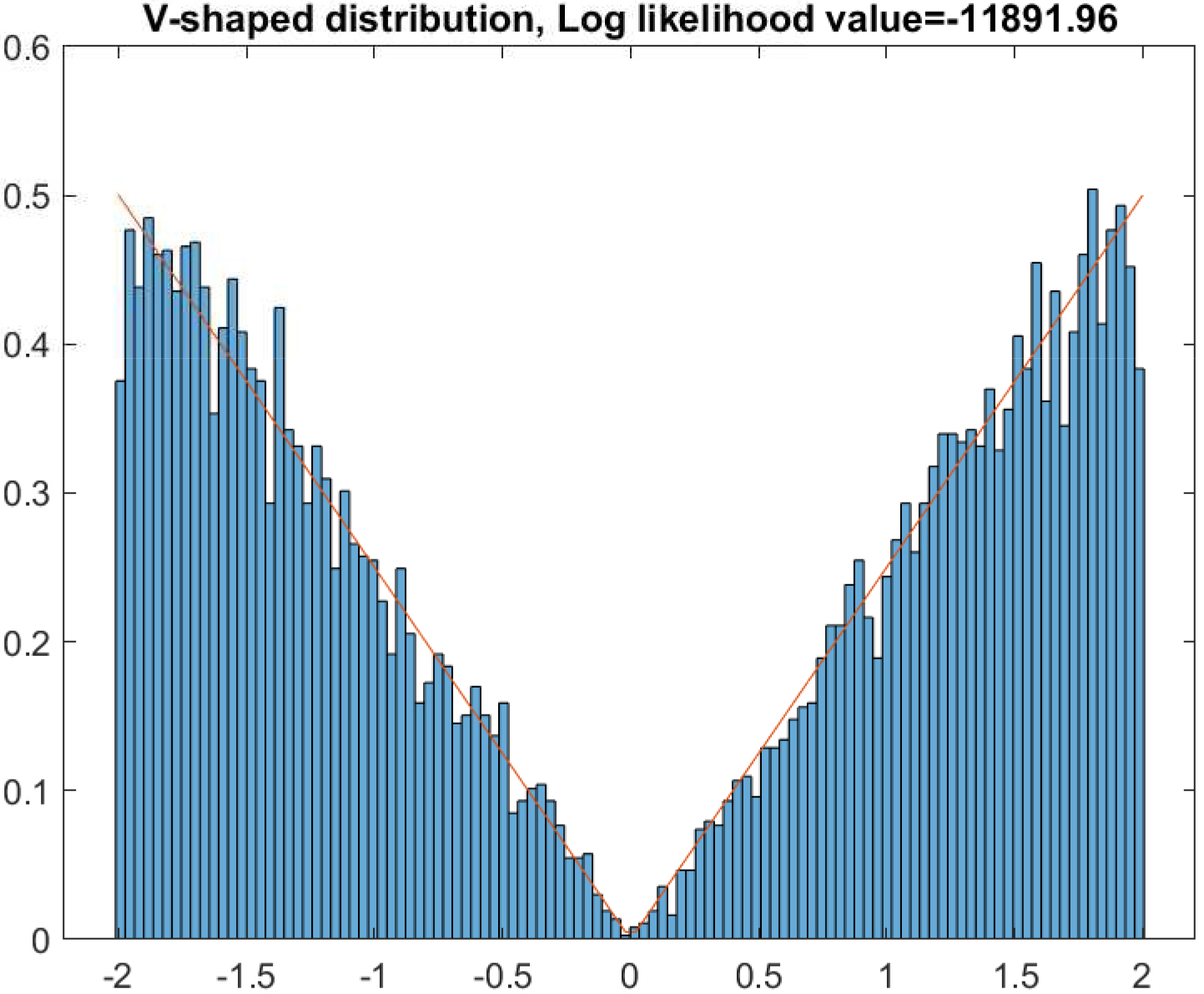
The histogram of the simulated data and the estimated asymmetric V-shaped distribution.

4. Numerical example

In this section, three examples are presented to illustrate the asymmetric V-shaped distribution. Example 1 extends Theorem 3.3 in such a way to generate any independent identically distributed (i.i.d.) uniform random variables $X,Y\sim \mathrm{U}(0,b)$ . Example 2 indicates the existence of the asymmetric V-shaped distribution when we establish the major error distribution of two measurements or two statistical/machine learning models. An application of the proposed distribution in analyzing the stock market behavior is depicted in Example 3. In each example, we compare the proposed distribution with the Gaussian distribution, the Beta distribution, the Gaussian mixture distribution, and the Arcsine distribution. The maximum likelihood estimation for each distribution is obtained using the quasi-Newton method. The obtained distributions are compared using the log-likelihood function.

4.1 Example 1

Let $X,Y$ have Uniform distributions on $[0,2]$ , $X,Y\sim \mathrm{U}(0,2)$ , we create a random variable $Z$ by $Z=\mathrm{sgn}(X-Y)\max \{X,Y\}$ . In this case, $Z$ is expected to follow the asymmetric V-shaped distribution, with $a=-2,m=0,b=2$ . Based on the Theorem 3.1, we can find the mean $\mathrm{E}(Z)$ , the median $\mathrm{Med}(Z)$ , and the variance $\mathrm{Var}(Z)$ as follows.

$\mathrm{E}(Z)={\displaystyle \frac{2b+2a-m}{3}}={\displaystyle \frac{2*(-2)+2*2-0}{3}}=0,$ $\mathrm{Med}(Z)=m-\sqrt{(m-a)\left(m-{\displaystyle \frac{a+b}{2}}\right)}=0-\sqrt{(0-(-2))\left(0-{\displaystyle \frac{(-2)+2}{2}}\right)}=0,$ $\mathrm{Var}(Z)={\displaystyle \frac{1}{18}}(b^2+a^2-7ab)-{\displaystyle \frac{5}{18}}m(m-a-b)$ $={\displaystyle \frac{1}{18}}(2^2+{(-2)}^2-7*(-2)*2)-{\displaystyle \frac{5}{18}}0(0-(-2)-2)=2.$

For determining the most suitable distribution, we first simulate 10000 pairs of $(X,Y)$ and then calculate the corresponding $Z$ . The maximum likelihood method is then applied for estimating the parameters of the Gaussian distribution, the Beta distribution, the Gaussian mixture distribution, the Arcsine distribution, and the asymmetric V-shaped distribution. Figure 3 depicts the histogram of the simulated data and the estimated asymmetric V-shaped distribution. The qualitative results in terms of log-likelihood values are summarized in Table 1. It can be seen from Table 1 that the most suitable distribution is the asymmetric V-shaped distribution, with $a=-1.9997,m=0,b=1.9996$ .

Table 1

The log-likelihood value of comparative distributions

Distribution	Log-likekihood value
Normal	$-$ 17661.9
Beta	$-$ 13111.2
Mixture Gaussian	$-$ 13489.3
Arcsine	$-$ 13402.2
Asymmetric V-shaped	$-$ 11892.0

We also further conduct similar experiments with $X,Y\sim \mathrm{U}(0,b)$ where $b$ is a positive number. The obtained result also indicates that the asymmetric V-shaped distribution is the most suitable distribution for those cases. Based on Theorem 3.3 and this example, it can be implied that if $X,Y\sim \mathrm{U}(0,b)$ then $Z=\mathrm{sgn}(X-Y)\max \{X,Y\}$ has the asymmetric V-shaped distribution $Z\sim \mathrm{aV}(-b,0,b)$ .

4.2 Example 2

Let $y=f(x)$ be the actual data value, $y_1=f_1(x)$ be the predicted value of Model 1, and $y_2=f_2(x)$ be the predicted value of Model 2. Let $e_1=y_1-y$ and $e_2=y_2-y$ be the corresponding errors of the two models, respectively. The major error of the two models is defined as $e^{*}={\arg }_{e_i}{\max }_i|e_i|$ . In other words, the major error of the two models is the error $e_i$ in $\{e_1,e_2\}$ such that its modulus is the maximum.

Figure 4.

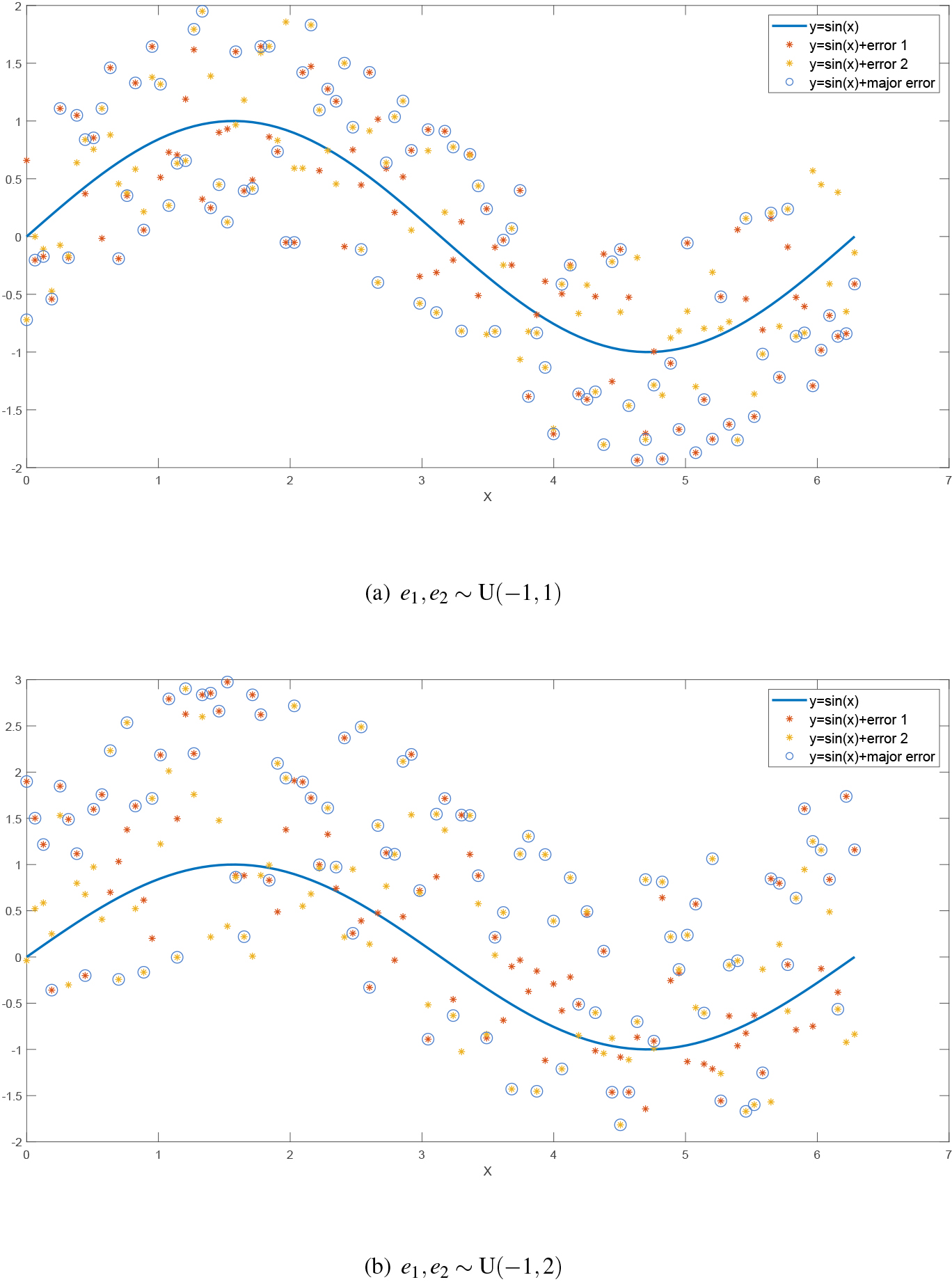
Illustrating for the major error.

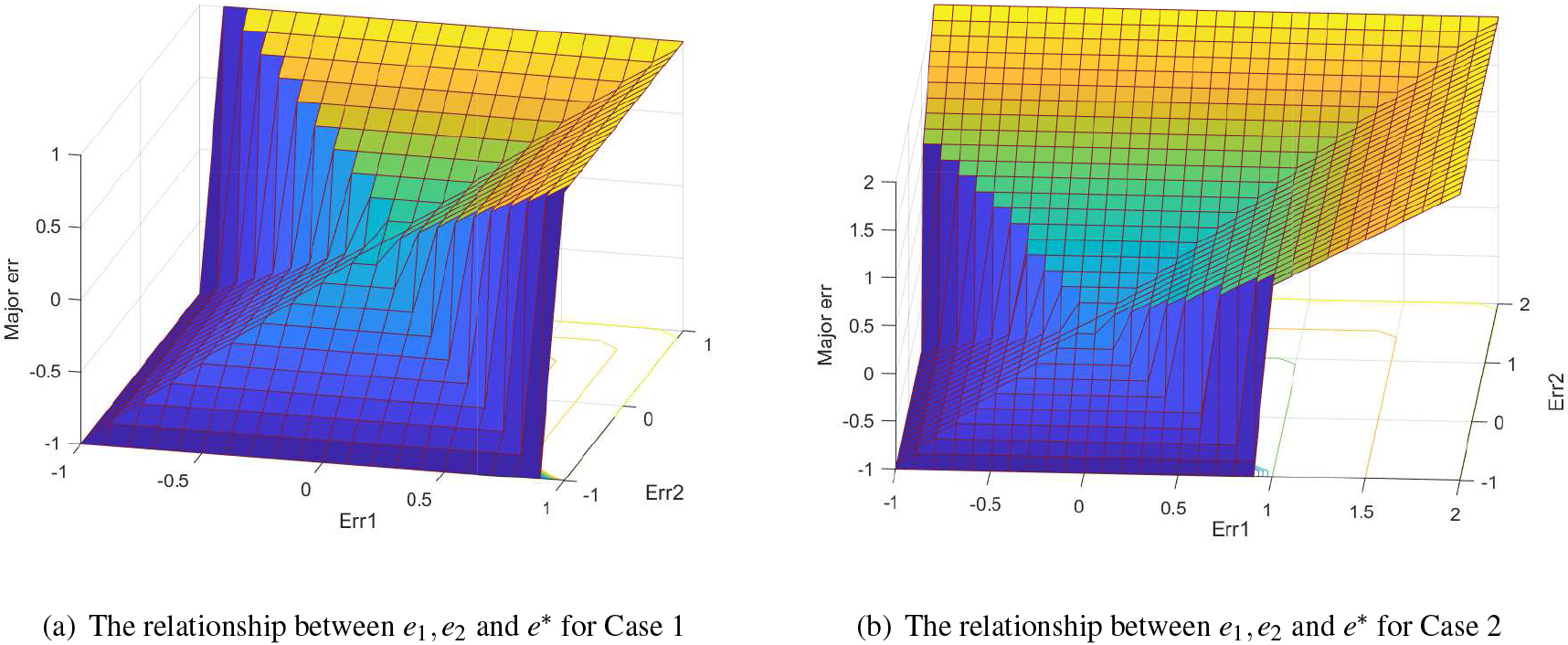
Figure 4 illustrates the major error. In Fig. 4, the blue line stands for the actual data $y=\sin (x)$ , the red points stand for the predicted values of Model 1 or $y_1{}_j=y_j+e_1{}_j$ , the yellow points stand for the predicted values of Model 2 or $y_2{}_j=y_j+e_2{}_j$ , the blue circle points stand for $y_j+e^{*}{}_j$ . It can be seen from Fig. 4 that the major error $e^{*}{}_j$ can be either $e_1{}_j$ or $e_2{}_j$ depending on their maximum value. The difference between Fig. 4a and b is that Fig. 4a stands for unbiased estimators (Case 1) when $e_1,e_2\sim \mathrm{U}(-1,1)$ ; whereas Fig. 4b stands for biased estimators (Case 2) $e_1,e_2\sim \mathrm{U}(-1,2)$ . We next consider the major error distribution in the two cases above. Similar to Example 1, we first simulate 10000 pairs of $(e_1{}_i,e_2{}_i)$ and then calculate the corresponding $e_i^{*}$ for each case. The relationships between $(e_1,e_2)$ and $e^{*}$ for two cases are given in Fig. 5. Obviously, in both cases, the surface area decreases as $e^{*}$ goes to zero. This will create a V-shaped distribution as we can see later. Furthermore, for Case 1 (unbiased estimators), the area of the surface where $e^{*}<0$ is equal to the area of the surface where $e^{*}>0$ . For case 2 (bias estimators), the area of the lower surface is smaller than the area of the upper surface leading to a strictly asymmetric property. Based on the above discussion, $e^{*}$ can potentially follow $\mathrm{aV}(-1,0,1)$ , and $\mathrm{aV}(-1,0,2)$ for the two cases. According to Theorem 3.1, $\mathrm{E}(e^{*})=0,\mathrm{Med}(e^{*})=0,\mathrm{Var}(e^{*})=\frac{1}{2}$ for Case 1 and $\mathrm{E}(e^{*})=\frac{2}{3},\mathrm{Med}(e^{*})=\sqrt{2},\mathrm{Var}(e^{*})=\frac{19}{18}$ for Case 2.

Figure 5.

The relationship between $e_1,e_2$ and $e^{*}$ for two cases.

Table 2

The log-likelihood value of comparative distributions

Distribution	Log-likelihood value
	Case 1	Case 2
Normal	$-$ 10724.1	$-$ 13322.3
Beta	$-$ 6180.0	$-$ 10262.0
Mixture Gaussian	$-$ 6566.0	$-$ 10411.6
Arcsine	$-$ 19960.7	$-$ 19722.9
Asymmetric V $-$ shaped	$-$ 4941.1	$-$ 9395.6

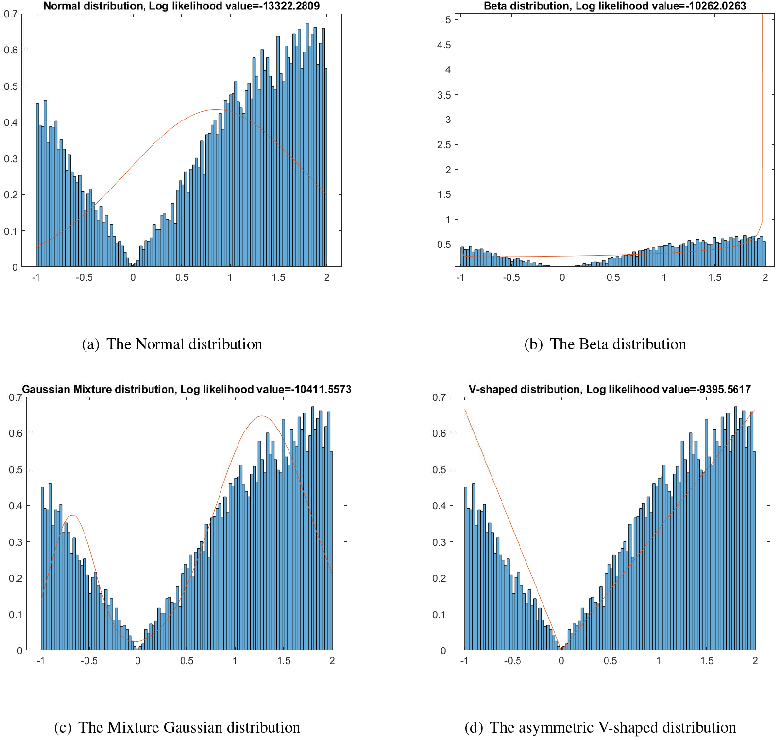
Similar to Example 1, the maximum likelihood method is applied for estimating the parameters of the comparative distributions. Some visualize results in the case of bias estimators are shown in Fig. 6, whereas the qualitative results in terms of log-likelihood values are summarized in Table 2.

As shown in Fig. 6 and Table 2, the asymmetric V-shaped distribution is the most suitable distribution for both cases, even if it is not too completely fit for the case of biased estimators. We also further conduct more experiments on various cases of $e_1$ and $e_2$ . The results show that if $e_1$ and $e_2$ are i.i.d uniform distribution, $e_1,e_2\sim \mathrm{U}(-|a|,|b|)$ , then the major error $e*$ has asymmetric V-shaped distribution, $e^{*}\sim \mathrm{aV}(-|a|,0,b)$ . It indicates the potential of asymmetric V-shaped distribution in modeling the major error distribution.

4.3 Example 3

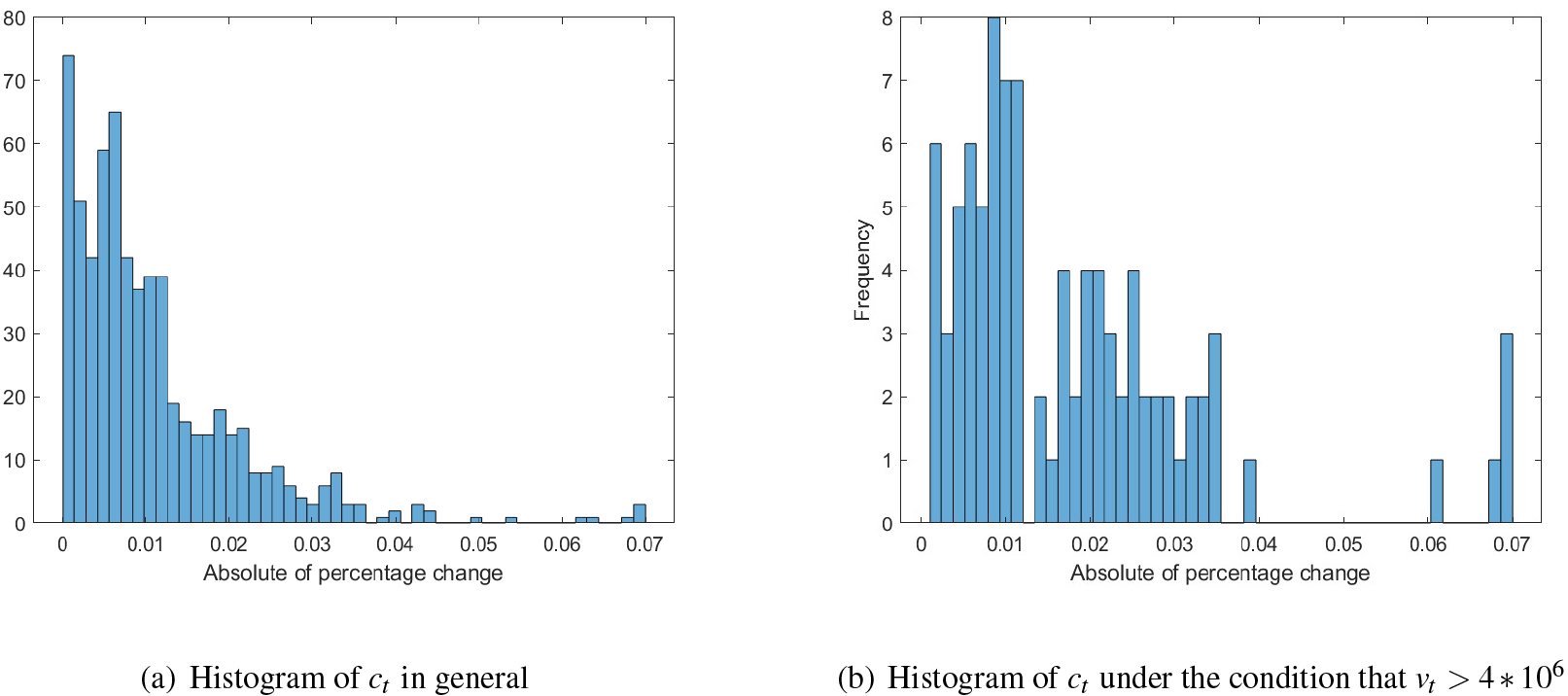
In this example, data from the Vietnam stock market are analyzed to demonstrate the applicability of the asymmetric V-shaped distribution to modeling fluctuations under certain conditions. To this end, the daily prices ( $x_t$ ) and volumes ( $v_t$ ) of specific equities are collected. The period under investigation is from 01/01/2021 to 18/07/2023. We then calculate the absolute of percentage change ( $c_t$ ) by $c_t=|x_t-x_{t-1}|/x_{t-1}$ .

Figure 7a illustrates the distribution of $c_t$ when examining the stock price of the Vietnam Dairy Products Joint Stock Company (VNM). It can be seen that the frequency of $c_t$ is concentrated between 0% and 1%, then non-linearly drops in the remainder of the range under consideration. This is typical behavior of stock price fluctuation that has been reported in previous studies (Yang & Zhang, 2019; Zebrowska-Suchodolska et al., 2021). However, this behavior does not hold when examining the fluctuations under different volume conditions. As shown in Fig. 7b, when $v_t>4*{10}^6$ , $c_t$ appears to follow an asymmetric V-shaped distribution. Specifically, the frequency of $c_t$ reaches its highest values in the range (0, 0.01), decreases linearly in the range (0.01, 0.065), and then increases abruptly in the range (0.065, 0.07). Using the maximum likelihood estimator, $\{c_t|v_t>4*{10}^6\}\sim \mathrm{aV}(0.001,0.067,0.070)$ can be calculated. Similar reports can be found when investigating some other individuals, such as the Asia Commercial Bank (ACB), the Vietnam Joint Stock Commercial Bank for Industry and Trade (CTG), and the Vietnam Prosperity Joint Stock Commercial Bank (VPB). Particularly,

•

$\{c_t|v_t>13.5*{10}^6\}\sim \mathrm{aV}(0,0.063,0.070)$ for ACB;

•

$\{c_t|v_t>15*{10}^6\}\sim \mathrm{aV}(0,0.067,0.070)$ for CTG;

•

$\{c_t|v_t>15*{10}^6\}\sim \mathrm{aV}(0,0.063,0.070)$ for VPB.

Table 3

The log-likelihood value of comparative distributions for some stocks

Distribution	Log-likelihood value
	ACB	CTG	VNM	VPB
Normal	232.2	315.5	256.6	177.4
Beta	253.4	348.4	279.7	195.2
Mixture Gaussian	253.1	335.1	275.9	191.9
Arcsine	244.1	337.9	268.9	191.3
Asymmetric V-shaped	259.3	355.8	287.5	196.4

Figure 6.

Some distributions using the maximum likelihood estimator.

Figure 7.

The histograms of the absolute percentage change.

Specific major results are summarized in Table 3. Table 3 shows that the asymmetric V-shaped distribution is the most appropriate one, compared to the other distributions. According to the above results, it can be seen that the distribution of $c_t$ will follow the asymmetric V-shaped distribution under certain conditions of $v_t$ . The value of the $v_t$ , which leads to the asymmetric V-shaped distribution of $c_t$ , also varies depending on the liquidity characteristics of each stock. As an explanation, it can be implied that the transaction liquidity has an effect on the price movement (Dong & Guo, 2022). Generally, higher volume leads to higher volatility. Specifically, as $v_t$ increases, the frequency of $c_t$ in the range (0, 0.01) decreases, while the frequency of $c_t$ in the range (0, 0.07) increases. Therefore, the nonlinear behavior of frequency $c_t$ is replaced by the linear behavior. As $c_t$ exceeds a specific threshold, e.g. 0.067 for VNM, herding behavior leads to a sharp increase in the frequency of $c_t$ . Additionally, the price range for shares is strictly limited in $\pm$ 7% for the Vietnam stock market, so $c_t>0.07$ is not the case. Those are the reasons why the absolute percentage change follows an asymmetric V-shaped distribution under a high value of volume.

In summary, the results obtained in this section have demonstrated the benefits of applying the asymmetric V-shaped distribution to specific numerical and real-world examples. Specifically, the proposed distribution can be used to represent the distribution of stock price fluctuations under a given volume condition. From our perspective, modeling stock price behaviors with the asymmetric V-shaped distribution is interesting and requires further investigation in future research.

5. Conclusion

This paper has proposed a new asymmetric V-shaped distribution. Some statistical properties of the new distribution have also been clarified. The numerical examples on simulated and actual data sets have been presented to illustrate the benefits of the proposed distribution in certain situations. In particular, the proposed distribution can represent the distribution of stock price fluctuations under conditions of high volume. This stock price behavior still requires further investigation. Additionally, related multivariate statistics and Bayesian statistics could be studied in the future.