Semi-analytical calculations of intrinsic field magnetic field inhomogeneities for a Neutron Spin Echo spectrometer at the ESS

Abstract

Neutron Spin Echo methods (NSE) use Larmor labelling to measure the precession phase of the neutron beam polarization around well-defined magnetic fields. Scattering by a sample can affect the resulting precession phase providing information on the sample’s structure and dynamics with high accuracy and resolution. A major limitation for the performance of Neutron Spin Echo instruments is the homogeneity of the precession magnetic fields. Here we investigate the influence of the new “pancake” moderator, which is being built at the European Spallation Source, on the design of a Neutron Spin Echo spectrometer. The calculations show clear gains when the height to width ratios of the rectangular beam cross-sections mimic those of the ESS “pancake” moderator beams. In such a case the homogeneity of the magnetic field integrals could improve by at least 30%. However, the calculations show that will not be possible to preserve a high resolution and at the same time reduce the length of the instrument. Consequently, NSE spectrometers will perform better at the ESS but they will not be substantially compacter than at other neutron sources e.g. ILL or FRM2.

1. Introduction

Most neutron scattering spectroscopic techniques determine separately the momentum and energy of the incident ( ${\overrightarrow{\mathit{k}}}_{\mathit{i}}$ , ${\mathit{ϵ}}_{\mathit{i}}$ ) and scattered beams ( ${\overrightarrow{\mathit{k}}}_{\mathit{s}}$ , ${\mathit{ϵ}}_{\mathit{s}}$ ) in order to deduce the momentum and energy transfer at the sample ( $\overrightarrow{\mathit{Q}}={\overrightarrow{\mathit{k}}}_{\mathit{i}}-{\overrightarrow{\mathit{k}}}_{\mathit{s}}$ , $\mathrm{\Delta }\mathit{ϵ}={\mathit{ϵ}}_{\mathit{i}}-{\mathit{ϵ}}_{\mathit{s}}$ ), which are the relevant parameters in neutron scattering. The relative accuracy in the determination of ${\overrightarrow{\mathit{k}}}_{\mathit{i}}$ . ${\mathit{ϵ}}_{\mathit{i}}$ , ${\overrightarrow{\mathit{k}}}_{\mathit{s}}$ and ${\mathit{ϵ}}_{\mathit{s}}$ also determines the lowest limit for $\mathrm{\Delta }|\overrightarrow{\mathit{Q}}|\mathrm{/}|\overrightarrow{\mathit{Q}}|$ and $\mathrm{\Delta }\mathit{ϵ}\mathrm{/}\mathit{ϵ}$ which can reach ${10}^{-3}$ , but with the cost of a high incident beam collimation and monochromatisation, and thus substantial intensity losses. In contrast, neutron spin echo methods use polarised neutrons and the precession of the neutron beam polarization $\overrightarrow{\mathit{P}}$ in a magnetic field $\overrightarrow{\mathit{B}}$ to directly measure the momentum and/or energy transfer at the sample. In this way, it is possible to decouple the momentum and energy resolution from beam characteristics like monochromatisation and collimation and reach the highest resolutions while keeping the high intensity advantage of poorly monochromatic and collimated beams [6]. For this purpose $\overrightarrow{\mathit{P}}$ should be non-collinear to $\overrightarrow{\mathit{B}}$ , in the optimal case the two vectors should be orthogonal to each other. In this case and in the weak magnetic fields commonly used in neutron scattering, $\overrightarrow{\mathit{P}}$ would precess around $\overrightarrow{\mathit{B}}$ following the classical equation of motion: $$\begin{array}{}\text{(1)}& \mathit{d}\overrightarrow{\mathit{P}}\mathrm{/}\mathit{d}\mathit{t}=-\mathit{\gamma }\mathrm{(}\overrightarrow{\mathit{P}}\times \overrightarrow{\mathit{B}}\mathrm{)}=\overrightarrow{\mathit{P}}\times {\overrightarrow{\mathit{\omega }}}_{\mathit{L}}\mathrm{,}\end{array}$$ where $\mathit{\gamma }=183.2\text{ rad}·\text{MHz}·{\text{T}}^{-1}$ is the neutron gyromagnetic ratio and ${\mathit{\omega }}_{\mathit{L}}$ the Larmor angular frequency. We note that this description is also quantum mechanically correct because $\overrightarrow{\mathit{P}}$ is an observable [7] and as such it follows the linear equations of motion of classical mechanics according to the Ehrenfest theorem.

A neutron beam characterised by the wavelength λ and the energy ϵ, has a velocity of $\text{v}=\mathit{h}\mathrm{/}\mathit{m}\mathit{\lambda }=\sqrt{2\mathit{ϵ}}\mathrm{/}\mathit{m}$ , with m the neutron mass and h the Planck constant. Thus, over a time lapse t it covers a distance $\ell =\text{v}\mathit{t}$ and, in a magnetic field perpendicular to its polarization vector, it accumulates a precession angle: $$\begin{array}{}\text{(2)}& \mathit{\phi }=|{\overrightarrow{\mathit{\omega }}}_{\mathit{L}}|\mathit{t}=\mathit{\gamma }\mathit{B}\ell \mathrm{/}\text{v}=\mathrm{(}\mathit{\gamma }\mathit{m}\mathrm{/}\mathit{h}\mathrm{)}\mathit{\lambda }·\mathit{B}·\ell =\mathit{\gamma }·\mathit{B}\ell \mathit{m}\mathrm{/}\sqrt{2\mathit{ϵ}}\mathrm{,}\end{array}$$ where B is the modulus of $\overrightarrow{\mathit{B}}$ . Therefore φ encodes both the energy ϵ and the trajectory ℓ of the beam. Most instruments measure the difference in precession angles accumulated before and after scattering, $\mathrm{\Delta }\mathit{\phi }={\mathit{\phi }}_{\mathit{i}}-{\mathit{\phi }}_{\mathit{s}}$ , and adopt magnetic field designs that disentangle the energy transfer contribution to $\mathrm{\Delta }\mathit{\phi }$ from the one arising from the momentum transfer, i.e. from the change of trajectories during the scattering process. SESANS instruments are designed to optimally encode momentum transfer [5,13], whereas NSE spectrometers should ideally encode only energy transfer. Thus NSE spectrometers are designed so that the precession phase is the same for all possible beam trajectories through the spectrometer. The relative precision requirements reach ${10}^{-6}$ , which for large beam cross sections pose stringent conditions on the magnetic field homogeneity. These are the major limiting factor for extending the NSE resolution beyond the state-of-the-art.

NSE spectrometers [4,9,10,15] measure the intermediate scattering function $\mathit{I}\mathrm{(}\overrightarrow{\mathit{Q}}\mathrm{,}\mathit{\tau }\mathrm{)}$ , where $\overrightarrow{\mathit{Q}}$ is the momentum transfer vector and τ the Fourier time given by: $$\begin{array}{}\text{(3)}& \mathit{\tau }=\hslash \mathrm{/}\mathrm{\left(}\mathit{m}{\text{v}}^3\mathrm{\right)}{\displaystyle \int }{\mathit{\omega }}_{\mathit{L}}\mathit{d}\ell ={\displaystyle \frac{1}{2\mathit{\pi }}}\mathit{\gamma }{\mathrm{\left(}{\displaystyle \frac{\mathit{m}}{\mathit{h}}}\mathrm{\right)}}^2{\mathit{\lambda }}^3{\displaystyle \int }\mathit{B}\mathit{d}\ell .\end{array}$$

The challenge in reaching the longest possible τ consists in realising high field integrals $\mathit{J}=\int \mathit{B}·\mathit{d}\ell$ with the highest possible homogeneity, thus with the smallest possible trajectory-dependence of $\mathrm{\Delta }\mathit{\phi }$ . In the following we will discuss the influence of some magnetic coil design parameters on the NSE modulation with focus on the repercussions the compact neutron beams emerging from the “pancake” moderators may have on an NSE spectrometer at the European Spallation Source. For this purpose we will consider the normalised NSE modulation, ${\mathit{P}}_{\mathrm{NSE}}$ , after precession in the spectrometer, either before (incoming beam) or after the sample (scattered beam). For ideally homogeneous magnetic fields ${\mathit{P}}_{\mathrm{NSE}}=1$ and magnetic field inhomogeneities obviously reduce ${\mathit{P}}_{\mathrm{NSE}}$ .

A Gauss distribution of magnetic field inhomogeneities will lead to a Gauss distribution of precession angles and to a decrease of ${\mathit{P}}_{\mathrm{NSE}}$ : $$\begin{array}{}\text{(4)}& {\mathit{P}}_{\mathrm{NSE}}\propto ⟨cos\mathrm{(}\mathrm{\Delta }\mathit{\phi }\mathrm{)}⟩=cos\mathrm{(}⟨\mathrm{\Delta }\mathit{\phi }⟩\mathrm{)}exp\mathrm{(}-{\mathrm{(}{\mathit{\sigma }}_{\mathrm{\Delta }\mathit{\phi }}\mathrm{)}}^2\mathrm{/}2\mathrm{)}=exp\mathrm{(}-{\mathrm{(}{\mathit{\sigma }}_{\mathrm{\Delta }\mathit{\phi }}\mathrm{)}}^2\mathrm{/}2\mathrm{)}\mathrm{,}\end{array}$$ where ${\mathit{\sigma }}_{\mathrm{\Delta }\mathit{\phi }}$ is the standard deviation for the Gaussian distribution of $\mathrm{\Delta }\mathit{\phi }$ , and $⟨\mathrm{\Delta }\mathit{\phi }⟩=0$ in spin-echo condition. We consider here the most general case of diffuse scattering, for which there is no correlation between the trajectories of the neutron beam before and after the sample.1

¹

The neutron beam trajectories before and after the sample are one-to-one correlated in the case of the direct beam (the part of the beam that has not been scattered by the sample) and the Bragg peaks. This feature is very important for the design and operation of SESANS [5,13] and Larmor diffraction [12] instruments.

In that case the variance of the sum of two normally distributed variables is the sum of individual variances, i.e. ${\mathit{\sigma }}_{\mathrm{\Delta }\mathit{\phi }}^2={\mathit{\sigma }}_{{\mathit{\phi }}_1}^2+{\mathit{\sigma }}_{{\mathit{\phi }}_2}^2$ . Using ${\mathit{J}}_0=\int |\mathit{B}|\mathit{d}\mathit{l}$ , the variance of the accumulated precession angle in one arm (either first or second) is $$\begin{array}{}\text{(5)}& {\mathit{\sigma }}_{\mathit{\phi }}^2={\mathrm{(}\mathit{m}\mathit{\gamma }\mathrm{/}\mathit{h}\mathrm{)}}^2{\mathit{\lambda }}^2⟨{\mathrm{(}{\mathit{J}}_0-\mathit{J}\mathrm{)}}^2⟩\end{array}$$ where J is the magnetic field integral along a specific trajectory and $⟨..⟩$ stands for the averaging over the neutron beam.

The longest Fourier time depends on the minimum acceptable spin-echo signal for an elastic scatterer. The decrease in the spin-echo signal is given by Eq. (4). As seen from Eq. (5), this decrease depends only on the wavelength and the field integral inhomogeneity, $\mathrm{\Delta }\mathit{J}=\sqrt{⟨{\mathrm{(}{\mathit{J}}_0-\mathit{J}\mathrm{)}}^2⟩}$ , for the first and second arm.

NSE spectrometers typically use longitudinal magnetic fields that are produced by solenoids, a configuration that reduces the intrinsic magnetic field integral inhomogeneities. Nonetheless, in order to reach Fourier times beyond several ns, Fresnel correction coils must be used, which reduce the magnetic field inhomogeneities by several order of magnitude [8]. However, as the performance of NSE spectrometers is pushed towards longer Fourier times, the Fresnel correction coils (classical circular or Pythagoras design) are often a limiting factor, due to the mechanical precision with which they can be manufactured and positioned in the instrument as well as due to the limited current density that can be used without overheating them. It is thus important to opt for a magnetic field design which reduces the intrinsic field integral inhomogeneities and this has been considered as a primary way to further optimise the NSE spectrometers and increase the accessible Fourier times.

The upgraded IN15 [3] as well as a proposal of a NSE spectrometer at the ESS [11] use coils with reduced intrinsic inhomogeneities based on a optimal field shape (OFS) solution suggested by Zeyen [17]. However, for comparable field integral inhomogeneities, the OFS solution requires the use of longer precession regions than simple solenoids. Indeed, for parallel neutron trajectories, the intrinsic field integral inhomogeneity for a solenoid is: [8] $$\begin{array}{}\text{(6)}& \mathrm{\Delta }{\mathit{J}}_{\mathrm{Sol}}={\mathit{r}}_0^2{\displaystyle \frac{{\mathit{J}}_0}{4\mathit{R}\mathit{L}}}\end{array}$$ where L and R are the length and radius of a solenoid, and ${\mathit{r}}_0$ is the radial coordinate. For an OFS solution the intrinsic field integral inhomogeneity becomes: $$\begin{array}{}\text{(7)}& \mathrm{\Delta }{\mathit{J}}_{\mathrm{OFS}}={\mathit{r}}_0^2{\displaystyle \frac{{\mathit{J}}_0}{2}}{\mathrm{\left(}{\displaystyle \frac{\mathit{\pi }}{\mathit{L}}}\mathrm{\right)}}^2\end{array}$$ where L is somewhat larger than the physical length of the coil. Hence, the OFS solution results in a lower inhomogeneity only for $\mathit{L}\mathrm{>}2\mathit{R}{\mathit{\pi }}^2$ . Thus, for a inner coil bore of 34 cm (as in J-NSE/SNS-NSE), the OFS coil length should be approx. 3.4 m, which is much longer than a typical main coil length (2 m for J-NSE, IN11, IN15). A longer instrument generally has lower neutron flux at the sample position. Therefore, for a high flux NSE spectrometer, a solenoid remains the first choice.

The magnetic field integral inhomogeneities arise from two sources: i) inhomogeneities of the magnetic field which lead to different precession angles for two parallel trajectories of the same length, and ii) beam divergence, which leads to trajectories with different lengths and thus with different precession angles even in a ideally homogeneous magnetic field. The separation of the effects of these two sources was considered by Zeyen [17] and, recently in more detail, by Pasini et al. [11].

In the following we will consider the separation of those two sources in a more general way and apply the results to assess the implications of the “pancake” moderator which is currently planned for the European Spallation Source (ESS) on an NSE instrument design [1,16]. The novelty of this moderator design is that it will produce high-intensity neutron beams over cross sections that are significantly smaller compared to research reactors. In other words, for the same intensity, averaged over time and the beam cross section, the neutron beams will have much smaller dimensions at the ESS than e.g. at the ILL or FRM2. When it comes to the NSE spectrometers first estimates lead to a beam height that can be as small as 1.5 cm, with a beam width reaching 6 cm. In the following we investigate the repercussion these smaller beam cross sections might have on the NSE instrument design. For this purpose, we considered a simple model case, which however catches the main characteristics of a NSE spectrometer. It turns out that irrespective of the choice of magnetic field layout, the use of a rectangular beam cross-section with a moderate aspect ratio of 1:4 (or larger), which mimics the dimensions of the ESS “pancake” moderator beams, reduces the field integral inhomogeneity in comparison to the square cross-sections. However, it will not be possible to preserve a high resolution and at the same time reduce the length of the instrument. Consequently, NSE spectrometers will perform better at the ESS but they will not be substantially compacter than at other neutron sources e.g. ILL or FRM2.

2. Separation of contributions due to magnetic layout and due to beam averages

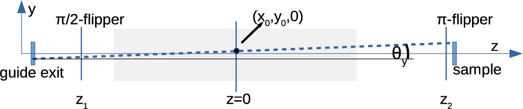
We start by defining a general layout of a precession region generated by solenoids as shown in Fig. 1. In this case, for a not too large neutron beam (i.e. when ${\mathit{B}}_{\mathit{r}}\mathrm{(}\mathit{z}\mathrm{,}\mathit{r}\mathrm{)}\Vert {\mathit{B}}_{\mathit{z}}\mathrm{(}\mathit{z}\mathrm{,}\mathit{r}\mathrm{)}$ , cf. p. 184 in [8]), the field integral J can be expressed as [11]: $$\begin{array}{}\text{(8)}& \mathit{J}=\sqrt{1+{tan}^2\mathit{\theta }}{{\displaystyle \int }}_{{\mathit{z}}_1}^{{\mathit{z}}_2}\mathit{d}\mathit{z}[{\mathit{B}}_{\mathit{z}}\mathrm{(}\mathit{z}\mathrm{)}+{|\overrightarrow{\mathit{r}}\mathrm{(}\mathit{z}\mathrm{)}|}^2\mathit{\beta }\mathrm{(}\mathit{z}\mathrm{)}]\end{array}$$ where ${\mathit{B}}_{\mathit{z}}\mathrm{(}\mathit{z}\mathrm{)}$ is the magnetic field on the z-axis and the function $\mathit{\beta }\mathrm{(}\mathit{z}\mathrm{)}$ is given by: $$\begin{array}{}\text{(9)}& \mathit{\beta }\mathrm{(}\mathit{z}\mathrm{)}={\displaystyle \frac{1}{8}}{\displaystyle \frac{1}{{\mathit{B}}_{\mathit{z}}\mathrm{(}\mathit{z}\mathrm{)}}}{\mathrm{\left(}{\displaystyle \frac{\partial {\mathit{B}}_{\mathit{z}}\mathrm{(}\mathit{z}\mathrm{)}}{\partial \mathit{z}}}\mathrm{\right)}}^2-{\displaystyle \frac{1}{4}}{\displaystyle \frac{{\partial }^2{\mathit{B}}_{\mathit{z}}\mathrm{(}\mathit{z}\mathrm{)}}{\partial {\mathit{z}}^2}}.\end{array}$$ The position of a neutron in the plane perpendicular to z-axis is specified by $\overrightarrow{\mathit{r}}\mathrm{(}\mathit{z}\mathrm{)}$ : $$\begin{array}{}\text{(10)}& \overrightarrow{\mathit{r}}\mathrm{(}\mathit{z}\mathrm{)}=\left(\begin{array}{c}\hfill {\mathit{x}}_0+\mathit{z}tan{\mathit{\theta }}_{\mathit{x}}\hfill \\ \hfill {\mathit{y}}_0+\mathit{z}tan{\mathit{\theta }}_{\mathit{y}}\hfill \end{array}\right)\mathrm{,}{\overrightarrow{\mathit{r}}}_0=\left(\begin{array}{c}\hfill {\mathit{x}}_0\hfill \\ \hfill {\mathit{y}}_0\hfill \end{array}\right)\end{array}$$ Thus, $\overrightarrow{\mathit{r}}\mathrm{(}\mathit{z}\mathrm{)}$ defines the trajectory of a neutron and ${\mathit{\theta }}_{\mathit{x}}$ and ${\mathit{\theta }}_{\mathit{y}}$ that are the angles between the z axis and the projections of the neutron trajectory on the $\mathit{x}\mathit{z}$ and $\mathit{y}\mathit{z}$ planes, respectively (see Fig. 1). The angle between the trajectory and the z-axis, θ, is defined by ${tan}^2\mathit{\theta }={tan}^2{\mathit{\theta }}_{\mathit{x}}+{tan}^2{\mathit{\theta }}_{\mathit{y}}$ . Equations (8), (10) are valid for any shape of a neutron beam and not only the radial symmetry implicitly assumed in Ref. [11]. Using Eq. (10) and $|{\mathit{r}}_0{|}^2={\mathit{x}}_0^2+{\mathit{y}}_0^2$ , we obtain: $$\begin{array}{}\text{(11)}& \hfill {|\overrightarrow{\mathit{r}}\mathrm{(}\mathit{z}\mathrm{)}|}^2={\mathrm{(}{\mathit{x}}_0+\mathit{z}tan{\mathit{\theta }}_{\mathit{x}}\mathrm{)}}^2+{\mathrm{(}{\mathit{y}}_0+\mathit{z}tan{\mathit{\theta }}_{\mathit{y}}\mathrm{)}}^2=|{\mathit{r}}_0{|}^2+{\mathit{z}}^2{tan}^2\mathit{\theta }+2\mathit{z}\mathrm{(}{\mathit{x}}_{0}tan{\mathit{\theta }}_{\mathit{x}}+{\mathit{y}}_{0}tan{\mathit{\theta }}_{\mathit{y}}\mathrm{)}& \end{array}$$

Fig. 1.

Schematic representation of a neutron trajectory, in the $\mathit{y}\mathit{z}$ plane, connecting the exit of the guide and the sample. The trajectory is defined by the point $\mathrm{(}{\mathit{x}}_0\mathrm{,}{\mathit{y}}_0\mathrm{)}$ and the angles ${\mathit{\theta }}_{\mathit{x}}$ (not shown) and ${\mathit{\theta }}_{\mathit{y}}$ between the z axis and the projections of the neutron trajectory on the $\mathit{x}\mathit{z}$ and $\mathit{y}\mathit{z}$ planes, respectively.

We use the same notations as Pasini et al. [11] and define the mean field integral: $$\begin{array}{}\text{(12)}& {\mathit{J}}_0={{\displaystyle \int }}_{{\mathit{z}}_1}^{{\mathit{z}}_2}\mathit{d}\mathit{z}{\mathit{B}}_{\mathit{z}}\mathrm{(}\mathit{z}\mathrm{)}\mathrm{,}\end{array}$$ the contribution from parallel trajectories: $$\begin{array}{}\text{(13)}& \mathit{H}={{\displaystyle \int }}_{{\mathit{z}}_1}^{{\mathit{z}}_2}\mathit{d}\mathit{z}\mathit{\beta }\mathrm{(}\mathit{z}\mathrm{)}\mathrm{,}\end{array}$$ the contribution due to divergence of the beam: $$\begin{array}{}\text{(14)}& \mathit{G}={\displaystyle \frac{{\mathit{J}}_0}{2}}+{{\displaystyle \int }}_{{\mathit{z}}_1}^{{\mathit{z}}_2}\mathit{d}\mathit{z}[{\mathit{z}}^2\mathit{\beta }\mathrm{(}\mathit{z}\mathrm{)}]\mathrm{,}\end{array}$$ and the cross-term: $$\begin{array}{}\text{(15)}& \mathit{U}={{\displaystyle \int }}_{{\mathit{z}}_1}^{{\mathit{z}}_2}\mathit{d}\mathit{z}\mathit{z}\mathit{\beta }\mathrm{(}\mathit{z}\mathrm{)}.\end{array}$$

Using Eq. (8), Eq. (11) and Eqs (12)–(15), the deviation from the field line integral, $\mathrm{\Delta }\mathit{J}=\mathit{J}-{\mathit{J}}_0$ , can be written as $$\begin{array}{}\text{(16)}& \hfill \mathrm{\Delta }\mathit{J}=\mathit{H}|{\mathit{r}}_0{|}^2+\mathit{G}{tan}^2\mathit{\theta }+2\mathit{U}[{\mathit{x}}_{0}tan{\mathit{\theta }}_{\mathit{x}}+{\mathit{y}}_{0}tan{\mathit{\theta }}_{\mathit{y}}]& \end{array}$$ Thus, the variance of the average over the neutron beam is given by: $$\begin{array}{ll}\hfill ⟨\mathrm{\Delta }{\mathit{J}}^2⟩=& {\mathit{H}}^2⟨|{\mathit{r}}_0{|}^4⟩+{\mathit{G}}^2⟨{tan}^4\mathit{\theta }⟩+2\mathit{H}\mathit{G}⟨|{\mathit{r}}_0{|}^2{tan}^2\mathit{\theta }⟩+4\mathit{H}\mathit{U}⟨|{\mathit{r}}_0{|}^2\mathrm{(}{\mathit{x}}_{0}tan{\mathit{\theta }}_{\mathit{x}}+{\mathit{y}}_{0}tan{\mathit{\theta }}_{\mathit{y}}\mathrm{)}⟩\\ \hfill & +4\mathit{G}\mathit{U}⟨{tan}^2\mathit{\theta }\mathrm{(}{\mathit{x}}_{0}tan{\mathit{\theta }}_{\mathit{x}}+{\mathit{y}}_{0}tan{\mathit{\theta }}_{\mathit{y}}\mathrm{)}⟩+4{\mathit{U}}^2[⟨{\mathit{x}}_0^2{tan}^2{\mathit{\theta }}_{\mathit{x}}⟩+⟨{\mathit{y}}_0^2{tan}^2{\mathit{\theta }}_{\mathit{y}}⟩\\ \text{(17)}& \hfill & +⟨2{\mathit{x}}_0{\mathit{y}}_{0}tan{\mathit{\theta }}_{\mathit{x}}tan{\mathit{\theta }}_{\mathit{y}}⟩].\end{array}$$

Equation (17) shows that it is possible to partially decouple effects of magnetic layout – which manifest themselves in the magnitude of H, G, U and effects of beam properties – which manifest themselves in several beam averages $⟨..⟩$ . As a general remark, the minimization of beam averages benefits to all magnetic layouts, solenoids or OFS.

Equation (16) and Eq. (17) are qualitatively similar to the Eq. (12), and Eq. (26), respectively, provided in the paper of Pasini et al. [11], with the difference that they are valid for any shape of a neutron beam. The contribution of one arm to the reduction of spin-echo amplitude is then given by: $$\begin{array}{}\text{(18)}& \mathit{R}=exp\mathrm{(}-{\mathrm{(}\mathrm{(}\mathit{m}\mathit{\gamma }\mathrm{/}\mathit{h}\mathrm{)}\mathit{\lambda }\mathrm{)}}^2⟨\mathrm{\Delta }{\mathit{J}}^2⟩\mathrm{/}2\mathrm{)}\end{array}$$

From Eq. (18), it is apparent that in order to reach longer Fourier times, one needs to minimize the intrinsic field integral inhomogeneity. For this purpose one must consider which terms contribute the most in Eq. (17), and how these can be minimised.

In the special case, where ${\mathit{z}}_1=-{\mathit{z}}_2$ , the integral U is zero, and Eq. (17) reduces to: $$\begin{array}{}\text{(19)}& ⟨\mathrm{\Delta }{\mathit{J}}^2⟩={\mathit{H}}^2⟨|{\mathit{r}}_0{|}^4⟩+{\mathit{G}}^2⟨{tan}^4\mathit{\theta }⟩+2\mathit{H}\mathit{G}⟨|{\mathit{r}}_0{|}^2{tan}^2\mathit{\theta }⟩\end{array}$$ From the comparison of Eq. (19) and Eq. (17), one can speculate that the symmetric magnetic layout leads to a lower field inhomogeneity. However, this is not necessarily the case, because U may be negative, and some of beam averages that come into the prefactors of $4{\mathit{U}}^2$ , $4\mathit{H}\mathit{U}$ , and $4\mathit{G}\mathit{U}$ may be negative as well. As a consequence, the sum of U-dependent terms may also be negative, and the net inhomogeneity of an asymmetric magnetic layout might be lower than that of the symmetric one. Therefore, in the following we will consider both symmetric and asymmetric magnetic layouts.

In Eq. (19), the prefactors ${\mathit{H}}^2$ , ${\mathit{G}}^2$ and $2\mathit{H}\mathit{G}$ , which depend on the specific magnetic layout, have different dimensions. In order to compare them with each other, we must thus bring them to the same dimensions, which we chose to be [length²]. This implies that we should compare ${\mathit{F}}_0={\mathit{H}}^2$ with ${\mathit{F}}_2=2\mathit{H}\mathit{G}\mathrm{/}{\mathit{L}}_{\mathrm{tot}}^2$ , and with ${\mathit{F}}_4={\mathit{G}}^2\mathrm{/}{\mathit{L}}_{\mathrm{tot}}^4$ . Under these considerations, Eq. (19) can be written as: $$\begin{array}{}\text{(20)}& ⟨\mathrm{\Delta }{\mathit{J}}^2⟩={\mathit{F}}_0⟨{\mathit{r}}_0^4⟩+{\mathit{F}}_2{\mathit{L}}_{\mathrm{tot}}^2⟨{\mathit{r}}_0^2{tan}^2\mathit{\theta }⟩+{\mathit{F}}_4{\mathit{L}}_{\mathrm{tot}}^4⟨{tan}^4\mathit{\theta }⟩\end{array}$$

3. Calculation details

The calculation of the field integral inhomogeneity, $\mathrm{\Delta }{\mathit{J}}_{\mathrm{RMS}}=\sqrt{⟨\mathrm{\Delta }{\mathit{J}}^2⟩}$ , from Eq. (17) requires the evaluation of the magnetic field integrals ${\mathit{J}}_0$ , H, G, U, and various beam averages, which will be addressed below.

Fig. 2.

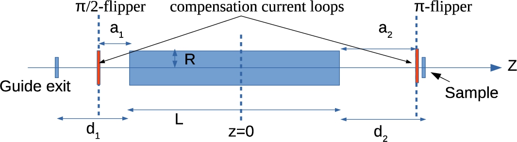
Schematic drawing of the first arm of a NSE spectrometer. The magnetic layout is characterized by the lengths L, ${\mathit{a}}_1$ , ${\mathit{a}}_2$ and the radius R. The beam size and divergence can be derived from the lengths L, ${\mathit{d}}_1$ , ${\mathit{d}}_2$ and the shape and size of the guide exit and sample respectively.

3.1. Magnetic field integrals

In order to evaluate the magnetic field integrals, one needs to calculate ${\mathit{B}}_{\mathit{z}}$ along the symmetry axis of the setup as well as its first and second derivatives with respect to z, cf. Eqs (12)–(15), which can be done by programs such as RADIA [2]. In this work, we assume the simple case of just one solenoid, the center of which is located at $\mathit{z}=0$ , as depicted in Fig. 2. In this case, ${\mathit{B}}_{\mathit{z}}$ can be written as: $$\begin{array}{}\text{(21)}& {\mathit{B}}_{\mathit{z}}^{\mathrm{SOL}}={\tilde{\mathit{B}}}_{\mathrm{SOL}}[{\displaystyle \frac{\mathit{L}\mathrm{/}2+\mathit{z}}{\sqrt{{\mathit{R}}^2+{\mathrm{(}\mathit{L}\mathrm{/}2+\mathit{z}\mathrm{)}}^2}}}+{\displaystyle \frac{\mathit{L}\mathrm{/}2-\mathit{z}}{\sqrt{{\mathit{R}}^2+{\mathrm{(}\mathit{L}\mathrm{/}2-\mathit{z}\mathrm{)}}^2}}}]\end{array}$$ where L is the coil length, R is the coil radius, and ${\tilde{\mathit{B}}}^{\mathrm{SOL}}$ is given by: $$\begin{array}{}\text{(22)}& {\tilde{\mathit{B}}}^{\mathrm{SOL}}={\mathit{\mu }}_0\mathit{I}\mathit{N}\mathrm{/}\mathrm{(}2\mathit{L}\mathrm{)}\mathrm{,}\end{array}$$ where I is the current and N the number of turns. In this case, the field integral becomes: $$\begin{array}{ll}\hfill {\mathit{J}}_0^{\mathrm{SOL}}=& {{\displaystyle \int }}_{{\mathit{z}}_1}^{{\mathit{z}}_2}{\mathit{B}}_{\mathit{z}}^{\mathrm{SOL}}\mathit{d}\mathit{z}={\tilde{\mathit{B}}}_{\mathrm{SOL}}[\sqrt{{\mathit{R}}^2+{\mathrm{(}\mathit{L}\mathrm{/}2+{\mathit{z}}_2\mathrm{)}}^2}-\sqrt{{\mathit{R}}^2+{\mathrm{(}\mathit{L}\mathrm{/}2+{\mathit{z}}_1\mathrm{)}}^2}\\ \text{(23)}& \hfill & +\sqrt{{\mathit{R}}^2+{\mathrm{(}\mathit{L}\mathrm{/}2-{\mathit{z}}_1\mathrm{)}}^2}-\sqrt{{\mathit{R}}^2+{\mathrm{(}\mathit{L}\mathrm{/}2-{\mathit{z}}_2\mathrm{)}}^2}]\end{array}$$

The lower and upper integral boundaries, ${\mathit{z}}_1$ and ${\mathit{z}}_2$ repsectively, for the magnetic field integral calculations are: $$\begin{array}{}\text{(24)}& {\mathit{z}}_1=-\mathrm{(}{\mathit{a}}_1+\mathit{L}\mathrm{/}2\mathrm{)}{\mathit{z}}_2=\mathrm{(}{\mathit{a}}_2+\mathit{L}\mathrm{/}2\mathrm{)}\end{array}$$ Thus, there are four relevant parameters for the setup: the length L, the radius R, and the distances ${\mathit{a}}_1$ , and ${\mathit{a}}_2$ . In addition, in order to be able to adjust the strength of the magnetic field at the positions of the $\mathit{\pi }\mathrm{/}2$ and π-flippers, we considered additional current loops located at ${\mathit{z}}_{\mathrm{loop}}={\mathit{z}}_1$ , and ${\mathit{z}}_{\mathrm{loop}}={\mathit{z}}_2$ . The field generated by such a current loop is given by: $$\begin{array}{}\text{(25)}& {\mathit{B}}_{\mathit{z}}^{\mathrm{loop}}={\displaystyle \frac{{\mathit{\mu }}_0{\mathit{I}}_{\mathrm{loop}}}{2{\mathit{R}}_{\mathrm{loop}}}}{\displaystyle \frac{1}{{[1+{\mathrm{(}\mathit{z}-{\mathit{z}}_{\mathrm{loop}}\mathrm{)}\mathrm{/}{\mathit{R}}_{\mathrm{loop}}\mathrm{)}}^2]}^{3\mathrm{/}2}}}\end{array}$$ where ${\mathit{R}}_{\mathrm{loop}}$ is the radius of the loop, and ${\mathit{I}}_{\mathrm{loop}}$ the current in the loop. For simplicity, we assume that the radius of the loop is the same as that of the solenoid. Consequently, the currents of the loops can be calculated from the conditions ${\mathit{B}}_{\mathit{z}}^{\mathrm{loop}}=-{\mathit{B}}_{\mathit{z}}^{\mathrm{SOL}}$ and $\mathit{d}{\mathit{B}}_{\mathit{z}}^{\mathrm{loop}}\mathrm{/}\mathit{d}\mathit{z}=-\mathit{d}{\mathit{B}}_{\mathit{z}}^{\mathrm{SOL}}\mathrm{/}\mathit{d}\mathit{z}$ .

The integrals of Eqs (13)–(15) were calculated using Mathematica^®, based on Eq. (21), Eq. (25) and ${\tilde{\mathit{B}}}^{\mathrm{SOL}}=1$ .

3.2. Beam averages

As it can be seen from the definition of θ in Section 2, the $tan\mathit{\theta }$ -averages depend on $$\begin{array}{}\text{(26)}& tan\mathit{\theta }=\sqrt{{tan}^2{\mathit{\theta }}_{\mathit{x}}+{tan}^2{\mathit{\theta }}_{\mathit{y}}}\mathrm{,}tan{\mathit{\theta }}_{\mathit{x}}={\displaystyle \frac{{\mathit{x}}_{\mathit{S}}-{\mathit{x}}_{\mathit{G}}}{{\mathit{d}}_1+\mathit{L}+{\mathit{d}}_2}}\mathrm{,}tan{\mathit{\theta }}_{\mathit{y}}={\displaystyle \frac{{\mathit{y}}_{\mathit{S}}-{\mathit{y}}_{\mathit{G}}}{{\mathit{d}}_1+\mathit{L}+{\mathit{d}}_2}}\end{array}$$ where ${\mathit{x}}_{\mathit{G}}\mathrm{,}{\mathit{y}}_{\mathit{G}}$ and ${\mathit{x}}_{\mathit{S}}\mathrm{,}{\mathit{y}}_{\mathit{S}}$ are coordinates that define the start and end of a neutron trajectory. Averages that involve $|\overrightarrow{{\mathit{r}}_0}|$ can be calculated using Eq. (10), which leads to: $$\begin{array}{}\text{(27)}& \overrightarrow{{\mathit{r}}_0}=\left(\begin{array}{c}\hfill {\mathit{x}}_0\hfill \\ \hfill {\mathit{y}}_0\hfill \end{array}\right)=\left(\begin{array}{c}\hfill {\mathit{x}}_{\mathit{G}}+tan{\mathit{\theta }}_{\mathit{x}}\mathrm{(}{\mathit{d}}_1+\frac{\mathit{L}}{2}\mathrm{)}\hfill \\ \hfill {\mathit{y}}_{\mathit{G}}+tan{\mathit{\theta }}_{\mathit{y}}\mathrm{(}{\mathit{d}}_1+\frac{\mathit{L}}{2}\mathrm{)}\hfill \end{array}\right).\end{array}$$ Here we define the symmetry parameter, s, which is a measure of how symmetrical the start and end of neutron tajectories are with respect to $\mathit{z}=0$ (i.e. with respect to the center of the magnetic layout) and is defined as: $$\begin{array}{}\text{(28)}& \mathit{s}=\mathrm{(}{\mathit{d}}_1+\mathit{L}\mathrm{/}2\mathrm{)}\mathrm{/}\mathrm{(}{\mathit{d}}_1+\mathit{L}+{\mathit{d}}_2\mathrm{)}\end{array}$$ Clearly, for ${\mathit{d}}_1={\mathit{d}}_2$ , $\mathit{s}=1\mathrm{/}2$ and using Eqs (26) and (28), Eq. (27) can be expressed as: $$\begin{array}{}\text{(29)}& \overrightarrow{{\mathit{r}}_0}=\left(\begin{array}{c}\hfill \mathrm{(}1-\mathit{s}\mathrm{)}{\mathit{x}}_{\mathit{G}}+\mathit{s}{\mathit{x}}_{\mathit{S}}\hfill \\ \hfill \mathrm{(}1-\mathit{s}\mathrm{)}{\mathit{y}}_{\mathit{G}}+\mathit{s}{\mathit{y}}_{\mathit{S}}\hfill \end{array}\right)\end{array}$$ Thus, beam averages depend only on the distances ${\mathit{d}}_1$ , and ${\mathit{d}}_2$ , the coil length L, and on the shape and size of the guide exit and the sample.

4. Results

4.1. Symmetric magnetic layout

We first consider the special case where ${\mathit{a}}_1={\mathit{a}}_2$ , i.e. the distance from one coil end to the first $\mathit{\pi }\mathrm{/}2$ -flipper ${\mathit{a}}_1$ is the same as the distance from the other coil end to the π-flipper. In this symmetric magnetic layout $\mathit{U}=0$ and Eq. (17) reduces to Eq. (19). Thus, there are only three relevant beam averages, $⟨|{\mathit{r}}_0{|}^4⟩$ , $⟨{tan}^4\mathit{\theta }⟩$ and $⟨|{\mathit{r}}_0{|}^2{tan}^2\mathit{\theta }⟩$ .

We also consider rectangular and circular cross-sections both for the guide exit and the sample. As can be seen from the general results provided in the Appendix A, the beam averages depend on the distance from the guide exit to the sample, and on the position of the main coil with respect to the start and end of neutron trajectories. For this reason, in the following we will first consider the symmetric setup, where $\mathit{s}=1\mathrm{/}2$ , and then discuss the general case.

4.1.1. Minimization of beam averages for a symmetric beam setup

The general expressions for the beam averages, $⟨{\mathit{r}}_0^4⟩$ , $⟨{\mathit{r}}_0^2{tan}^2\mathit{\theta }⟩$ , and $⟨{tan}^4\mathit{\theta }⟩$ , are provided in the Appendix A, Eqs (A.1), (A.2), and (A.3) for rectangular cross-sections, and by Eqs (A.5), (A.6), and (A.7) for circular one. These are valid for any value of the symmetry parameter s. The three relevant beam averages, $⟨{\mathit{r}}_0^4⟩$ , $⟨{\mathit{r}}_0^2{tan}^2\mathit{\theta }⟩{\mathit{L}}_{\mathrm{tot}}^2$ and $⟨{tan}^4\mathit{\theta }⟩{\mathit{L}}_{\mathrm{tot}}^4$ in Eq. (20) for the symmetric beam setup ( $\mathit{s}=1\mathrm{/}2$ ) are provided in the upper part of Table 1 as a function of the beam cross-section shape and size. First, we consider the case where the sample size is approximately equal to that of the guide exit, and for simplicity, we assume that the sizes are exactly the same. The results show that, irrespective of the relative importance of the three terms that contribute to Eq. (20), a rectangular cross-section with an aspect ratio (height to width ratio) of 1:4 leads to a lower $⟨\mathrm{\Delta }{\mathit{J}}^2⟩$ by a factor at least 2.7 with respect to the square cross-section.

Similar results are obtained in the case where the sample size is much smaller than that of the guide exit, as shown in the lower part of Table 1. Also in this case, a change of the aspect ratio from 1:1 to 1:4 leads to a decrease in the beam averages by at least a factor of 3. The trend persists also in the case, where the sample size is much larger than the size of the guide exit. These results are not shown in Table 1 because they are exactly the same as for the previous case, provided ${\mathit{A}}_{\mathit{G}}\mathrm{,}{\mathit{B}}_{\mathit{G}}$ and ${\mathit{R}}_{\mathit{G}}$ in the lower part of Table 1 are substituted by ${\mathit{A}}_{\mathit{S}}\mathrm{,}{\mathit{B}}_{\mathit{S}}$ and ${\mathit{R}}_{\mathit{S}}$ .

Table 1

Beam averages calculated for the symmetric beam setup ( $\mathit{s}=1\mathrm{/}2$ ) and the two special cases, where the size of the sample is the same as that of the guide exit, and where the sample size is much smaller than the size of the guide

Averages & conditions	Guide shape
	Rectangle	“pancake” ( ${\mathit{B}}_{\mathit{G}}\to 0$ )	${\mathit{B}}_{\mathit{G}}={\mathit{A}}_{\mathit{G}}\mathrm{/}4$	Square ( ${\mathit{B}}_{\mathit{G}}={\mathit{A}}_{\mathit{G}}$ )	Circle
Sample size is the same as of the guide exit	${\mathit{A}}_{\mathit{S}}={\mathit{A}}_{\mathit{G}}\mathrm{,}{\mathit{B}}_{\mathit{S}}={\mathit{B}}_{\mathit{G}}$				${\mathit{R}}_{\mathit{S}}={\mathit{R}}_{\mathit{G}}$
$⟨{\mathit{r}}_0^4⟩$	$\frac{6{\mathit{A}}_{\mathit{G}}^4+5{\mathit{A}}_{\mathit{G}}^2{\mathit{B}}_{\mathit{G}}^2+6{\mathit{B}}_{\mathit{G}}^4}{90}$	0.067 ${\mathit{A}}_{\mathit{G}}^4$	0.070 ${\mathit{A}}_{\mathit{G}}^4$	0.189 ${\mathit{A}}_{\mathit{G}}^4$	0.1042 ${\mathit{R}}_{\mathit{G}}^4$
${\mathit{L}}_{\mathrm{tot}}^2⟨{\mathit{r}}_0^2{tan}^2\mathit{\theta }⟩$	$\frac{2{\mathit{A}}_{\mathit{G}}^4+10{\mathit{A}}_{\mathit{G}}^2{\mathit{B}}_{\mathit{G}}^2+2{\mathit{B}}_{\mathit{G}}^4}{45}$	0.044 ${\mathit{A}}_{\mathit{G}}^4$	0.058 ${\mathit{A}}_{\mathit{G}}^4$	0.311 ${\mathit{A}}_{\mathit{G}}^4$	0.1667 ${\mathit{R}}_{\mathit{G}}^4$
${\mathit{L}}_{\mathrm{tot}}^4⟨{tan}^4\mathit{\theta }⟩$	$\frac{8\mathrm{(}6{\mathit{A}}_{\mathit{G}}^4+5{\mathit{A}}_{\mathit{G}}^2{\mathit{B}}_{\mathit{G}}^2+6{\mathit{B}}_{\mathit{G}}^4\mathrm{)}}{45}$	1.07 ${\mathit{A}}_{\mathit{G}}^4$	1.13 ${\mathit{A}}_{\mathit{G}}^4$	3.02 ${\mathit{A}}_{\mathit{G}}^4$	1.67 ${\mathit{R}}_{\mathit{G}}^4$
Sample is much smaller than the guide exit	${\mathit{A}}_{\mathit{S}}\to 0\mathrm{,}{\mathit{B}}_{\mathit{S}}\to 0$				${\mathit{R}}_{\mathit{S}}\to 0$
$⟨{\mathit{r}}_0^4⟩$	$\frac{9{\mathit{A}}_{\mathit{G}}^4+10{\mathit{A}}_{\mathit{G}}^2{\mathit{B}}_{\mathit{G}}^2+9{\mathit{B}}_{\mathit{G}}^4}{720}$	0.0125 ${\mathit{A}}_{\mathit{G}}^4$	0.0134 ${\mathit{A}}_{\mathit{G}}^4$	0.0389 ${\mathit{A}}_{\mathit{G}}^4$	0.0208 ${\mathit{R}}_{\mathit{G}}^4$
${\mathit{L}}_{\mathrm{tot}}^2⟨{\mathit{r}}_0^2{tan}^2\mathit{\theta }⟩$	$\frac{9{\mathit{A}}_{\mathit{G}}^4+10{\mathit{A}}_{\mathit{G}}^2{\mathit{B}}_{\mathit{G}}^2+9{\mathit{B}}_{\mathit{G}}^4}{180}$	0.05 ${\mathit{A}}_{\mathit{G}}^4$	0.054 ${\mathit{A}}_{\mathit{G}}^4$	0.156 ${\mathit{A}}_{\mathit{G}}^4$	0.0833 ${\mathit{R}}_{\mathit{G}}^4$
${\mathit{L}}_{\mathrm{tot}}^4⟨{tan}^4\mathit{\theta }⟩$	$\frac{9{\mathit{A}}_{\mathit{G}}^4+10{\mathit{A}}_{\mathit{G}}^2{\mathit{B}}_{\mathit{G}}^2+9{\mathit{B}}_{\mathit{G}}^4}{45}$	0.2 ${\mathit{A}}_{\mathit{G}}^4$	0.215 ${\mathit{A}}_{\mathit{G}}^4$	0.622 ${\mathit{A}}_{\mathit{G}}^4$	0.3333 ${\mathit{R}}_{\mathit{G}}^4$

4.1.2. Minimization of beam averages for an asymmetric beam setup

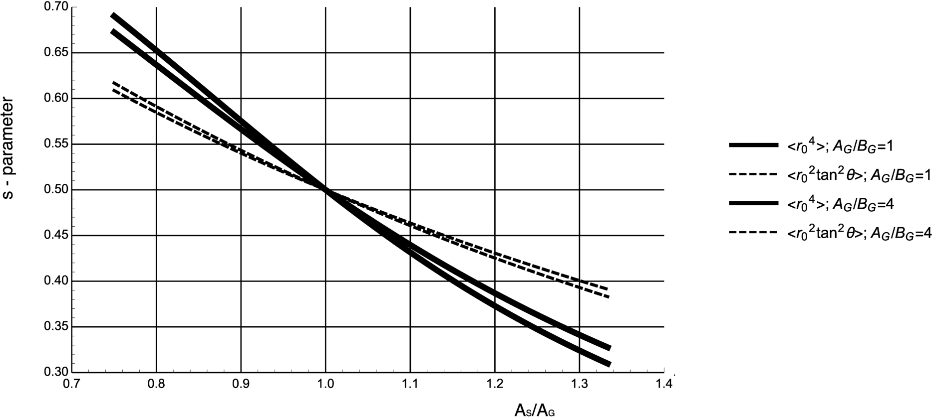
If the sample size is the same as that of the guide exit, the minima in $⟨{\mathit{r}}_0^4⟩$ and $⟨{\mathit{r}}_0^2{tan}^2\mathit{\theta }⟩$ both occur for $\mathit{s}=1\mathrm{/}2$ , irrespective of the aspect ratio of the guide exit. However, in general, the optimum s-values are not the same for $⟨{\mathit{r}}_0^4⟩$ and $⟨{\mathit{r}}_0^2{tan}^2\mathit{\theta }⟩$ , and depend on the relative size of the sample and the guide exit, as illustrated by the example shown in Fig. 3. Thus, the optimum s-parameter depends on the sample size and this affects the overall optimisation of the magnetic field integral.

Fig. 3.

Optimal s-parameter obtained by minimising the beam averages, $⟨{\mathit{r}}_0^4⟩$ and $⟨{\mathit{r}}_0^2{tan}^2\mathit{\theta }⟩$ . The aspect ratio of the guide exit is ${\mathit{A}}_{\mathit{G}}\mathrm{/}{\mathit{B}}_{\mathit{G}}$ , and is equal to that of the sample, i.e. ${\mathit{A}}_{\mathit{S}}\mathrm{/}{\mathit{A}}_{\mathit{G}}={\mathit{B}}_{\mathit{S}}\mathrm{/}{\mathit{B}}_{\mathit{G}}$ .

In practice, the geometry of the NSE spectrometers is fixed. Nonetheless, it may be possible to increase s by increasing ${\mathit{d}}_1$ , e.g. by removing the last section of the guide. However, it is much more difficult to reduce s as this would require either a decrease of the guide exit – coil distance or an increase of the coil end – sample distance. The alternative and easier to implement solution would be to decrease the dimensions of the guide exit in order to match those of smaller samples instead of modifying s. This however, would lead to a substantial reduction of the neutron flux.

For a specific instrument geometry, the good compromise for the value of the s-parameter may result from the minimum of $⟨{\mathit{r}}_0^4⟩$ derived for the specific guide exit cross-section and size, and for the most typical sample size to be used. That is, from ${\mathit{A}}_{\mathit{S}}\mathrm{,}{\mathit{B}}_{\mathit{S}}\mathrm{,}{\mathit{A}}_{\mathit{G}}\mathrm{,}{\mathit{B}}_{\mathit{G}}$ , one can calculate s, and then, based on the coil length L, the only remaining free parameters are the distances from the coil ends to the guide exit and the sample. To illustrate this we consider the case where instead of matching the sample to the guide dimensions, with ${\mathit{A}}_{\mathit{G}}\mathrm{/}{\mathit{B}}_{\mathit{G}}=4$ , ${\mathit{A}}_{\mathit{S}}={\mathit{A}}_{\mathit{G}}\mathrm{,}{\mathit{B}}_{\mathit{S}}={\mathit{B}}_{\mathit{G}}$ , and $\mathit{s}=1\mathrm{/}2$ , one uses a sample with half the guide dimensions ( ${\mathit{A}}_{\mathit{S}}={\mathit{A}}_{\mathit{G}}\mathrm{/}2\mathrm{,}{\mathit{B}}_{\mathit{S}}={\mathit{B}}_{\mathit{G}}\mathrm{/}2$ ) while keeping other parameters the same. In this case, the optimum value of s is $\approx 0.85$ and for $\mathit{s}=1\mathrm{/}2$ the average $⟨{\mathit{r}}_0^4⟩$ is about 2.5 times larger than for the optimum s. Similar differences are found for other ${\mathit{A}}_{\mathit{G}}$ : ${\mathit{B}}_{\mathit{G}}$ -ratios.

In the next section, we consider the contributions from the intrinsic magnetic field inhomogeneity and show that for a solenoid, it is more important to minimize $⟨{\mathit{r}}_0^4⟩$ than $⟨{\mathit{r}}_0^2{tan}^2\mathit{\theta }⟩$ .

4.1.3. Minimization of intrinsic magnetic field inhomogeneity

In principle, the length of the magnetic layout, which is ${\mathit{a}}_1+\mathit{L}+{\mathit{a}}_2$ , is slightly different from ${\mathit{L}}_{\mathrm{tot}}={\mathit{d}}_1+\mathit{L}+{\mathit{d}}_2$ . However, in practice the differences can be neglected. Indeed, the π-flipper is usually located very close to the sample, which leads to ${\mathit{a}}_2\approx {\mathit{d}}_2$ . Furthermore, the first $\mathit{\pi }\mathrm{/}2$ -flipper is also located very close to the guide exit, so that ${\mathit{a}}_1\approx {\mathit{d}}_1$ . Thus, ${\mathit{L}}_{\mathrm{tot}}$ is approximately the same as the length of the magnetic layout.

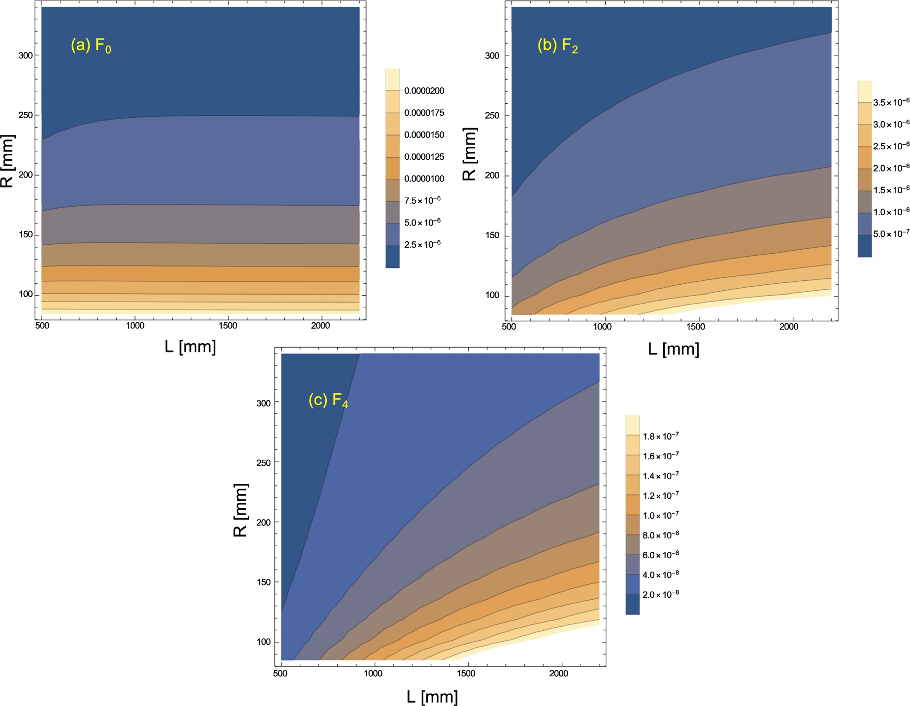
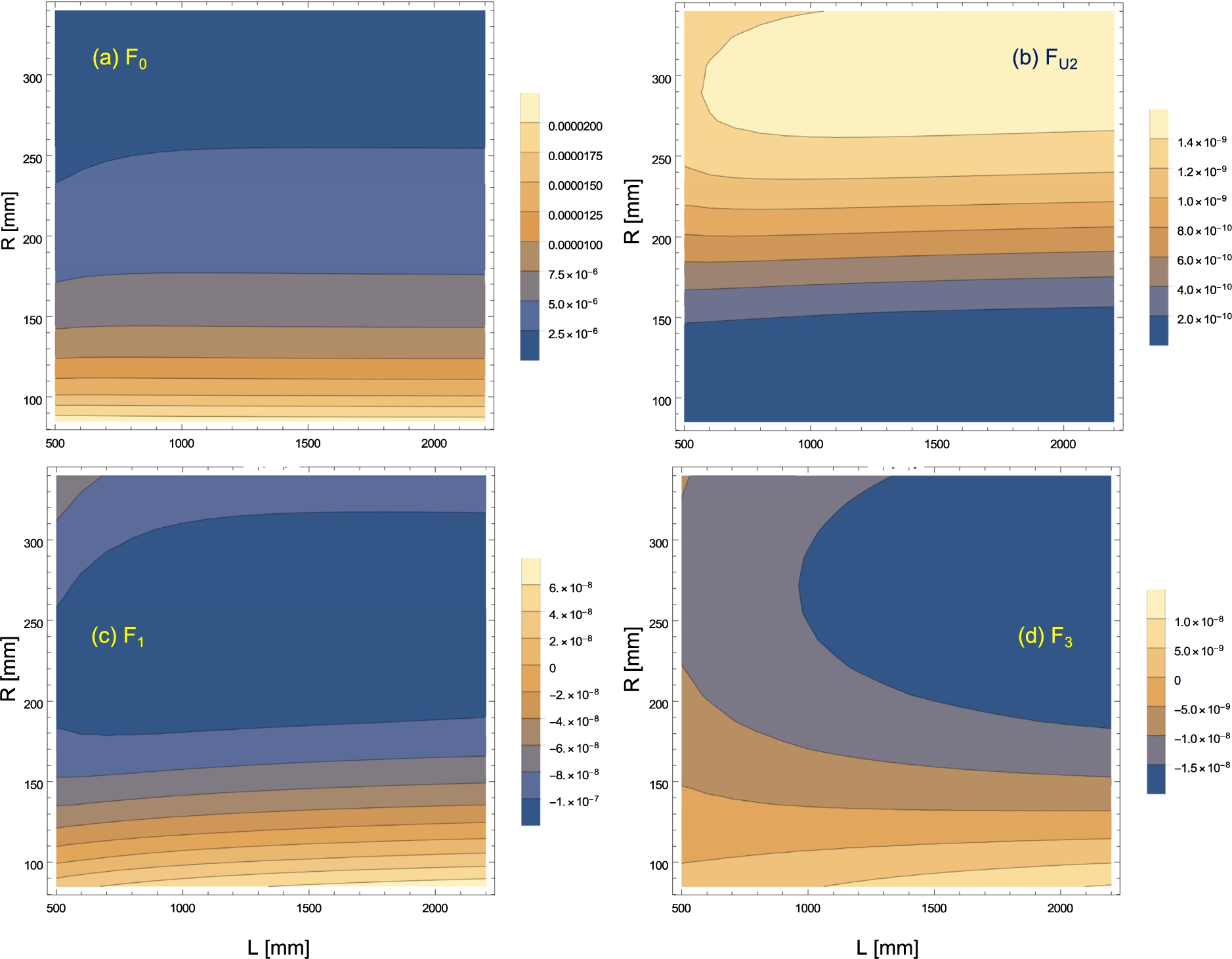
The beam averages were discussed in the previous section and in the following we will look at their pre-factors in Eq. (20). We evaluated ${\mathit{F}}_0$ , ${\mathit{F}}_2$ , and ${\mathit{F}}_4$ for ${\mathit{a}}_1={\mathit{a}}_2=0.5$ m and the results are shown in Fig. 4. In this calculation, the two compensation current loops were used, which leads to a minor correction with respect to the case where these loops are omitted.

Fig. 4.

Calculated magnetic layout-dependent contributions to $⟨\mathrm{\Delta }{\mathit{J}}^2⟩$ : a) ${\mathit{F}}_0={\mathit{H}}^2$ (due to the beam size), b) ${\mathit{F}}_2=\frac{2\mathit{H}\mathit{G}}{{\mathit{L}}_{\mathrm{tot}}^2}$ (due to the beam size and divergence), and C) ${\mathit{F}}_4=\frac{{\mathit{G}}^2}{{\mathit{L}}_{\mathrm{tot}}^4}$ (due to divergence only).

${\mathit{F}}_2$ is about 5 times lower than ${\mathit{F}}_0$ . From Table 1, one can see that for square or circular cross sections, of comparable dimensions for the sample and the guide exit, ${\mathit{L}}_{\mathrm{tot}}^2⟨{\mathit{r}}_0^2{tan}^2\mathit{\theta }⟩\propto 1.6⟨{\mathit{r}}_0^4⟩$ , which implies that ${\mathit{F}}_2{\mathit{L}}_{\mathrm{tot}}^2⟨{\mathit{r}}_0^2{tan}^2\mathit{\theta }⟩\approx 0.3{\mathit{F}}_0⟨{\mathit{r}}_0^4⟩$ . On the other hand, when the sample size is much smaller (or much larger) than the guide exit size, ${\mathit{L}}_{\mathrm{tot}}^2⟨{\mathit{r}}_0^2{tan}^2\mathit{\theta }⟩\mathrm{/}⟨{\mathit{r}}_0^4⟩\approx 4$ and ${\mathit{F}}_2{\mathit{L}}_{\mathrm{tot}}^2⟨{\mathit{r}}_0^2{tan}^2\mathit{\theta }⟩\approx 0.8{\mathit{F}}_0⟨{\mathit{r}}_0^4⟩$ .

${\mathit{F}}_4$ is approximately two orders of magnitude smaller than ${\mathit{F}}_0$ . As can be seen from Table 1, irrespective of the relation between the sample size and the guide exit size, ${\mathit{L}}_{\mathrm{tot}}^4⟨{tan}^4\mathit{\theta }⟩\mathrm{/}⟨{\mathit{r}}_0^4⟩\approx 15$ . Thus, ${\mathit{F}}_4{\mathit{L}}_{\mathrm{tot}}^4⟨{tan}^4\mathit{\theta }⟩$ is only about 15 % of ${\mathit{F}}_0⟨{\mathit{r}}_0^4⟩$ .

Thus, for a solenoid, the major contribution to $⟨\mathrm{\Delta }{\mathit{J}}^2⟩$ is always ${\mathit{F}}_0⟨{\mathit{r}}_0^4⟩$ , which is due solely to the size of the beam. However, as can been in Fig. 4a, this term is almost independent of the coil length, although it depends on the coil radius, and the estimate of $⟨\mathrm{\Delta }{\mathit{J}}^2⟩$ by Eq. (6), for ${\mathit{J}}_0\approx 2\mathit{L}$ (assuming ${\mathit{a}}_1={\mathit{a}}_2$ , cf. Eq. (23)), leads to: $⟨\mathrm{\Delta }{\mathit{J}}^2⟩\propto 1\mathrm{/}\mathrm{(}2\mathit{R}\mathrm{)}$ .

The other terms reduce slightly the absolute field inhomogeneities for shorter coils. However, as the mean field integral is proportional to the coil length, the relative field integral inhomogeneity will be lower (i.e. better) for longer coils.

4.2. Asymmetric magnetic layout

In general, the magnetic layouts of the NSE instruments are not necessarily symmetric. For example, the distance between the first $\mathit{\pi }\mathrm{/}2$ -flipper and the first main coil may be shorter than the distance between the main coil and the π-flipper, which is located in front of the sample. The opposite situation is unlikely because of the extra space around the sample, which is typically reserved for the sample environment. Thus, in general, the contributions to $⟨\mathrm{\Delta }{\mathit{J}}^2⟩$ from $4{\mathit{U}}^2$ , $4\mathit{H}\mathit{U}$ , and $4\mathit{G}\mathit{U}$ (cf. Eq. (19)) may be significant. As mentioned above, in order to compare these contributions with each other, we brought them to the same dimensions of [length²]. In the following we therefore compare ${\mathit{F}}_0={\mathit{H}}^2$ with ${\mathit{F}}_1=4\mathit{H}\mathit{U}\mathrm{/}{\mathit{L}}_{\mathrm{tot}}$ , ${\mathit{F}}_3=4\mathit{G}\mathit{U}\mathrm{/}{\mathit{L}}_{\mathrm{tot}}^3$ , and ${\mathit{F}}_{\mathit{U}2}=4{\mathit{U}}^2\mathrm{/}{\mathit{L}}_{\mathrm{tot}}^2$ . These terms are calculated for the case of a weak asymmetry, with ${\mathit{a}}_1=$ 0.3 m, and ${\mathit{a}}_2=$ 0.5 m and plotted as a function of the coil radius and length in Fig. 5. The results show that ${\mathit{F}}_0={\mathit{H}}^2$ is the dominant term. Among the other terms, the most significant term is ${\mathit{F}}_1=4\mathit{H}\mathit{U}\mathrm{/}{\mathit{L}}_{\mathrm{tot}}$ , which however is about 20 times weaker than that of ${\mathit{F}}_0$ .

We note that beam averages of $4{\mathit{U}}^2$ are always positive, but beam average of $4\mathit{H}\mathit{U}$ and $4\mathit{G}\mathit{U}$ may be positive or negative, depending on the beam setup symmetry, s, and the relation between the guide exit and sample size (see Appendix B). Thus, its is possible to find a combination of parameters where the $4\mathit{H}\mathit{U}$ and $4\mathit{G}\mathit{U}$ terms lower the total $⟨\mathrm{\Delta }{\mathit{J}}^2⟩$ . However, it is not clear whether this effect would be significant. On addition, when considering more asymmetric magnetic layouts (with a larger difference between ${\mathit{a}}_1$ , and ${\mathit{a}}_2$ ), one can reach more negative $4\mathit{H}\mathit{U}$ and $4\mathit{G}\mathit{U}$ , but it is not clear whether such setups would correspond to a realistic situation. Thus, it appears that an asymmetric magnetic layout does not bring significant benefits but also no significant drawbacks: the absolute magnitudes of the U-dependent contributions are probably too small and, as a consequence, they have little effect on $⟨\mathrm{\Delta }{\mathit{J}}^2⟩$ .

Fig. 5.

Calculated magnetic layout-dependent contributions for an asymmetric magnetic layout ( ${\mathit{a}}_1$ = 0.3 m, and ${\mathit{a}}_2$ = 0.5 m). a) ${\mathit{F}}_0={\mathit{H}}^2$ (due to the beam size), b) ${\mathit{F}}_{\mathit{U}2}=4{\mathit{U}}^2\mathrm{/}{\mathit{L}}_{\mathrm{tot}}^2$ , c) ${\mathit{F}}_1=4\mathit{H}\mathit{U}\mathrm{/}{\mathit{L}}_{\mathrm{tot}}$ , and d) ${\mathit{F}}_3=4\mathit{G}\mathit{U}\mathrm{/}{\mathit{L}}_{\mathrm{tot}}^3$ . In panels c and d, $\mathit{H}\mathit{U}$ and $\mathit{G}\mathit{U}$ are negative for small ${\mathit{H}}^2$ -values, but when ${\mathit{a}}_1\mathrm{>}{\mathit{a}}_2$ , their sign is reversed (results not shown).

5. Conclusion

Before moving to the conclusions, it is important to note that our calculations involve only the first arm of an NSE spectrometer. Nonetheless, all considerations can also be applied for the second arm and the magnetic fields after the sample. An important difference, however, is that detector size is much larger than that of the sample. This is analogous to the case of a guide exit much smaller than the size of the sample and the results obtained in this case can be applied. In this respect we note that all existing instruments have adopted a symmetric configuration with the same coil geometry before and after the sample. However, if the difference between the guide and detector dimensions exceeds the present “standard”, as it might be the case at a future NSE instrument at the ESS, one might consider adopting a non-symmetric setup with a different magnetic field optimisation before and after the sample. On the other hand, as the layout of the instrument will not be fundamentally affected by the reduced incoming beam dimensions, one may consider “expanding” the neutron beam cross-section in the vertical direction, by inserting a “polarising-all-neutrons” device in the beam delivery system [14], and thus partly restore the symmetry between the two arms of the spectrometer while benefiting from a higher neutron flux.

The semi-analytical magnetic field calculations discussed above show that a circular shape for the sample and the guide exit leads to lower field integral inhomogeneity in comparison to a square one. However, in practice, guides usually have square or rectangular cross-sections and so do the detectors. Using circular beam masks would lead to a loss of flux. By choosing rectangular cross-sections with a moderate aspect ratio, e.g. 1:4, one can reach even smaller beam averages than for circular shape.

Consequently, there is a clear gain with the “pancake” moderator beams. Indeed, rectangular beam cross-sections with a height over width ratio, e.g. 1:4, that mimic the ESS “pancake” moderator beams lead to the best results, and improve the homogeneity of the magnetic field integrals. On the other hand, because relative inhomogeneities become worse for shorter coils, in order to reach high resolution, i.e. long Fourier times, the length of the instruments cannot be reduced. NSE spectrometers should perform better at the ESS, but they will not be more compact than e.g. at the ILL or FRM2.