Outlier detection using conditional information entropy and rough set theory

Abstract

Outlier detection is critically important in the field of data mining. Real-world data have the impreciseness and ambiguity which can be handled by means of rough set theory. Information entropy is an effective way to measure the uncertainty in an information system. Most outlier detection methods may be called unsupervised outlier detection because they are only dealt with unlabeled data. When sufficient labeled data are available, these methods are used in a decision information system, which means that the decision attribute is discarded. Thus, these methods maybe not right for outlier detection in a a decision information system. This paper proposes supervised outlier detection using conditional information entropy and rough set theory. Firstly, conditional information entropy in a decision information system based on rough set theory is calculated, which provides a more comprehensive measure of uncertainty. Then, the relative entropy and relative cardinality are put forward. Next, the degree of outlierness and weight function are presented to find outlier factors. Finally, a conditional information entropy-based outlier detection algorithm is given. The performance of the given algorithm is evaluated and compared with the existing outlier detection algorithms such as LOF, KNN, Forest, SVM, IE, and ECOD. Twelve data sets have been taken from UCI to prove its efficiency and performance. For example, the AUC value of CIE algorithm in the Hayes data set is 0.949, and the AUC values of LOF, KNN, SVM, Forest, IE and ECOD algorithms in the Hayes data set are 0.647, 0.572, 0.680, 0.676, 0.928 and 0.667, respectively. The advantage of the proposed outlier detection method is that it fully utilizes the decision information.

1 Introduction

Outlier detection, also known as anomaly detection, refers to the identification of rare items, events or observations which difer from the general distribution of a population [43]. Outlier detection has many applications, such as insurance claim fraud detection [2, 17], fraud detection in finance [3, 12], network intrusion detection [8, 34], intelligent transportation development [11], health diagnosis [16, 29].

Based on the availability of labels in the training data sets, the existing outlier detection methods can be classified into 3 categories: unsupervised methods, semi-supervised methods,and supervised methods [20]. Supervised methods use labeled data to train an outlier detection model. Semi-supervised methods for anomaly detection aim to utilize a small pool of labeled samples. Since a labeled instance is difficult to obtain, most existing techniques are unsupervised, which can work with unlabeled data [1, 5]. Supervised anomaly detection techniques are superior in performance compared to unsupervised anomaly detection techniques since these techniques use labeled samples [15].

Degirmenci et al. [8] put forward efficient density and cluster based incremental outlier detection in data streams. Din et al. [11] exploited evolving microclusters for data stream classification with emerging class detection. Domingues et al. [10] gave a comparative evaluation of outlier detection algorithms. Du et al. [13] raised graph autoencoderbased unsupervised outlier detection. Kandanaarachchi et al. [21] brought up unsupervised anomaly detection ensembles using item response theory. Liu et al. [23] invoked data adaptive functional outlier detection. Wang et al. [36] provided outlier detection using weighted neighbourhood information network for mixed-valued datasets. Yuan et al. [38] researched outlier detection using fuzzy rough granules in mixed attribute data. Yuan et al. [39] studied hybrid data-driven outlier detection using neighborhood information entropy and its developmental measures. Jin et al. [18] introduced intrusion detection on internet of vehicles via combining log-ratio oversampling, outlier detection and metric learning. Meira et al. [26] came up with fast anomaly detection with locality-sensitive hashing and hyperparameter autotuning. Wang et al. [37] advanced autonomous hyperspectral anomaly detection network using fully convolutional autoencoder. Zhuang et al. [42] investigated hyperspectral image denoising and anomaly detection based on low-rank and sparse representations. Zhang et al. [45] considered outlier detection using three-way neighborhood characteristic regions and corresponding fusion measurement. Gao et al. [14] introduced a relative granular ratio-based outlier detection method in heterogeneous data.

Rough set theory (RST), proposed by Pawlak [27], is a mathematical tool to handle imprecision, vagueness and uncertainty. RST is widely used in feature selection [7, 23], and pattern recognition [25].

Methods for anomaly detection based on RST have been studies, and these methods have be showed better effectiveness and adaptability in detecting outliers. Jiang et al. [19, 20] proposed an outlier detection method using approximation accuracy entropy using rough set. Yuan et al. [39] introduced outlier detection using neighborhood information entropy according to the hybrid data-driving, Yuan et al. [38] extended fuzzy information entropy-based adaptive method for mixed feature outlier detection, which can applicable data sets widely concern categorical, numeric, and mixed data.

Many researchers have applied Shannon’s information entropy to rough sets [30]. By now, the mechanism for measuring uncertainty in rough sets based on Shannon’s information entropy has been formed [6, 44]. Furthermore, Singh [31, 32] gave a general model of ambiguous sets to a single-valued ambiguous numbers with aggregation operators and investigated ambiguous sets with application to decision-making from partial order to lattice ambiguous sets.

Most of the aforementioned outlier detection methods are unsupervised because they are only dealt with unlabeled data. If sufficient labeled data are available and these methods are used in a decision information system (DIS), then this means that the decision attribute is discarded and leads to information loss. Thus, these methods are not suitable for detecting the outliers in a DIS. In this paper, a supervised method for outlier detection using conditional entropy and rough set theory is proposed, and the conditional information entropy-based outlier detection algorithm is designed. The advantage of the proposed supervised method is that it fully utilizes the decision information. The main contributions are summarized as follows.

(1) Based on the rich theoretical knowledge of RST, the conditional information entropy, relative entropy and relative cardinality in a DIS are proposed, which to some extent enriches the application scenarios and scope of information entropy.

(2) In order to find outlier factors, the degree of outlierness and weight function are put forward. An outlier detection algorithm using conditional information entropy is presented. The experimental results show that the presented algorithm has better validity and adaptability for a DIS.

The rest of this paper is organized as follows. Binary relations and information entropy in a DIS are reviewed in Section 2. A conditional information entropy-based method using rough set theory is proposed in Section 3. Experiments and comparisons on UCI data sets are conducted in Section 4. The conclusion is given in Section 5. The work process of this paper is shown in Fig. 1.

Fig. 1

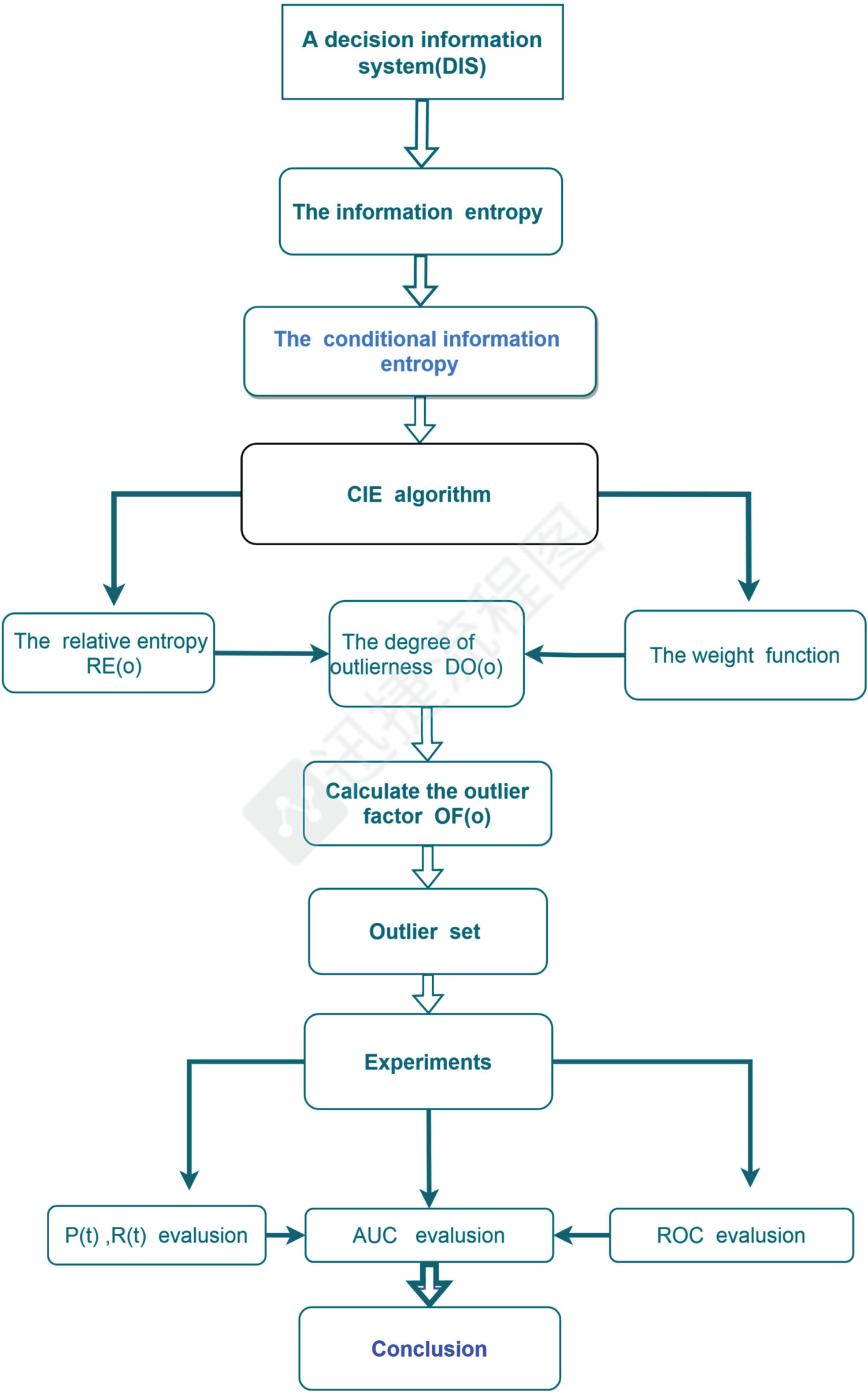
The work flow of this paper.

2 Preliminaries

We first look back at binary relations and information entropy in a DIS.

Throughout this paper, O denotes a finite sets, 2 ^O represents the power set of O and |X| is the cardinality of X ∈ 2 ^O . Put

$O=\{o_1,\cdots ,o_n\}.$(1)

2.1 Binary relations

Recall that R is a binary relation on O whenever R ⊆ O × O.

(1) R is called reflexive, if (o, o) ∈ R for any o ∈ O;

(2) R is called symmetric, if (o, o′) ∈ R implies (o′, o) ∈ R;

(3) R is called transitive, if (o, o′) ∈ R and (o′, o″) ∈ R imply (o, o″) ∈ R.

R is said to be an equivalence relation on O, if R is reflexive, symmetric and transitive; R is called a tolerance relation on O, if R is reflexive and symmetric.

2.2 Information entropy in a DIS

Definition 2.1. [27] Let O be an object set and A an attribute set. Suppose that O and A are finite sets. Then (O, A) is called an information system (IS), if each attribute a determines an information function a : O → V _a , where V _a  = {a (o) : o ∈ O}.

(O, C, d) is known as a decision information system (DIS), if (O, C ∪ {d}) is an IS, where C denotes a set of conditional attributes and d a decision attribute. If P ⊆ C, then (O, P, d) is referred to as the subsystem of (O, C, d).

Let (O, C, d) be a DIS. For any P ⊆ C, define ind (P) = {(o, o′) ∈ O × O : ∀  a ∈ P,  a (o) = a (o′)} , $R_d=\left\{\right(o,o^{\prime })\in O\times O:d(o)=d(o^{\prime }\left)\right\}.$(2)

Clearly, ind (P) and R _d are two equivalence relations on O.

Denote $[o{]}_P=\{o^{\prime }\in O:(o,o^{\prime })\in \mathit{ind}\left(P\right)\},$(3) $R_d\left(o\right)=\{o^{\prime }\in O:(o,o^{\prime })\in R_d\}.$(4) Then [o]  _P is called the equivalence class of the object o under the equivalence relation ind (P), and R _d  (o) is called the decision class of the object o. Put O/ind (d) = {R _d  (o) : o ∈ O} = {D₁, D₂, ⋯ , D _r } .

Proposition 2.2. Let (O, C, d) be a DIS. If P₁ ⊆ P₂ ⊆ C, then ∀ o ∈ O, $[o{]}_{P_2}\subseteq [o{]}_{P_1}.$

Proof. Obviously. □

Definition 2.3. [19] Let (O, C) be an IS with O = {o₁, ⋯ , o _n } and P ⊆ C. Suppose that O/ind (P) = {X₁, X₂, ⋯ , X _M }. Then information entropy H (P) of the subsystem (O, C) is defined as $H\left(P\right)=-\sum _{i=1}^M\frac{\left|X_i\right|}{n}{log}_2\frac{\left|X_i\right|}{n}.$(5)

Proposition 2.4. Let (O, C) be an IS with O = {o₁, ⋯ , o _n } and P ⊆ C. Then $H\left(P\right)=-\sum _{i=1}^n\frac{1}{n}{log}_2\frac{\left|\right[o_i{]}_P|}{n}.$(6)

Proof. Denote $O/\mathit{ind}\left(P\right)=\{X_1,X_2,\dots ,X_M\}.$

Suppose that $X_i=\{o_{i1},o_{i2},\dots ,o_{{\mathit{is}}_i}\}$ then |X _i | = s _i . So $\sum _{i=1}^M{s}_i=n,X_i=[o_{i1}{]}_P=[o_{i2}{]}_P=\cdots =[o_{{\mathit{is}}_i}{]}_P.$

This implies that $\left|X_i\right|=\left|\right[o_{i1}{]}_P|=|\left[o_{i2}{]}_P\right|=\cdots =\left|\right[o_{{\mathit{is}}_i}{]}_P|=s_i.$

Thus ∀ i, $\begin{array}{cc}\hfill \frac{\left|X_i\right|}{n}{log}_2\frac{\left|X_i\right|}{n}& =s_i\frac{1}{n}{log}_2\frac{\left|X_i\right|}{n}\hfill \\ \hfill & =\sum _{k=1}^{s_i}\frac{1}{n}{log}_2\frac{\left|\right[o_{\mathit{ik}}{]}_P|}{n}\hfill \\ \hfill & \hfill \end{array}$

Hence $\begin{array}{cc}\hfill H\left(P\right)& =-\sum _{i=1}^M\frac{\left|X_i\right|}{n}{log}_2\frac{\left|X_i\right|}{n}\hfill \\ \hfill & =-\sum _{i=1}^M\sum _{k=1}^{s_i}\frac{1}{n}{log}_2\frac{\left|\right[o_{\mathit{ik}}{]}_P|}{n}\hfill \\ \hfill & =-\sum _{i=1}^n\frac{1}{n}{log}_2\frac{\left|\right[o_i{]}_P|}{n}.\hfill \end{array}$

Similarly, conditional information entropy of a DIS is defined as follows.

Definition 2.5. For a DIS (O, C, d), let P ⊆ C, the conditional information entropy of P to d is defined as $H\left(P\right|d)=-\sum _{i=1}^n\sum _{j=1}^r\frac{1}{n}{log}_2\frac{\left|\right[o_i{]}_P\cap D_j|}{\left|\right[o_i{]}_P|}.$(7)

Definition 2.6. For a DIS (O, C, d), let P ⊆ C, then the joint information entropy of P and d is defined as $H(P\cup d)=-\sum _{i=1}^n\sum _{j=1}^r\frac{1}{n}{log}_2\frac{\left|\right[o_i{]}_P\cap D_j|}{n}.$(8)

Proposition 2.7. For a DIS (O, C, d), let P ⊆ C, then $H\left(P\right|d)=H(P\cup d)-H(P).$(9)

Proof. $\begin{array}{cc}\hfill H\left(P\right|d)& =-\sum _{i=1}^n\sum _{j=1}^r\frac{1}{n}({log}_2\frac{\left|\right[o_i{]}_P\cap D_j|}{n}\hfill \\ \hfill & -{log}_2\frac{\left|\right[o_i{]}_P|}{n})\hfill \\ \hfill & =-\sum _{i=1}^n\sum _{j=1}^r\frac{1}{n}{log}_2\frac{\left|\right[o_i{]}_P\cap D_j|}{n}\hfill \\ \hfill & +\sum _{i=1}^n\sum _{j=1}^r\frac{1}{n}{log}_2\frac{\left|\right[o_i{]}_P|}{n}\hfill \\ \hfill & =H(P\cup d)-H\left(P\right).\hfill \end{array}$

Propositions 2.7 indicates that Definition 2.5 is reasonable.

3 Outlier detection in a DIS using conditional information entropy

This section studies outlier detection in a DIS using conditional information entropy. In order to detect outliers in rough sets, based on the concept of conditional information entropy defined above, we propose a new concept: relative conditional entropy, which gives a measure of uncertainty for each object in the domain O.

For a DIS (O, C, d), let P ⊆ C and x ∈ O, put $\begin{array}{cc}\hfill & O_P^x=O-[x{]}_P=\{x_1,x_2,\cdots ,x_s\},\hfill \\ \hfill & {\mathit{ind}}^x\left(P\right)=\left\{\right(o,o^{\prime })\in O_P^x\times O_P^x:\forall a\in P,a(o)=a(o^{\prime }\left)\right\},\hfill \\ \hfill & R_d^x\left(P\right)=\left\{\right(o,o^{\prime })\in O_P^x\times O_P^x:d(o)=d(o^{\prime }\left)\right\}.\hfill \\ \hfill & R_d^x\left(P\right)\left(o\right)=\{o^{\prime }\in O_P^x:(o,o^{\prime })\in R_d^x(P\left)\right\}.\hfill \\ \hfill & O_P^x/\mathit{ind}\left(d\right)=\left\{R_d^x\right(P\left)\right(o):o\in O_P^x\}=\{F_1,F_2,\cdots ,F_l\},\hfill \\ \hfill & \hfill \end{array}$ Given any P ⊆ C and x ∈ O, when we delete all objects in equivalence class ind (P) of x from O, if the conditional information entropy of knowledge ind (P) varies little or even increases, then we may consider the uncertainty of object x under ind (P) is low or even equals 0. On the other hand, if the conditional information entropy of knowledge ind (P) decreases greatly, then we may consider the uncertainty of object x under ind (P) is high.

Definition 3.1. For a DIS (O, C, d), let P ⊆ C and x ∈ O, define the conditional information entropy of knowledge ind (P) when removing all objects [x]  _P in ind (P) from O. $\begin{array}{cc}\hfill & H_x\left(P\right|d)=-\sum _{i=1}^s\sum _{j=1}^l\frac{1}{s}{log}_2\frac{\left|\right[x_i{]}_P^x\cap F_j|}{\left|\right[x_i{]}_P^x|}.\hfill \\ \hfill & \hfill \end{array}$(10) Since the aim of outlier detection is to find the small groups of objects in O who behave in an unexpected way or have abnormal properties. And uncertainty can be deemed as a kind of abnormal property [19].

Definition 3.2. (Relative Conditional Entropy) For a DIS (O, C, d), let P ⊆ C and x ∈ O, define ${\mathit{RE}}_P^d\left(x\right)=\{\begin{array}{ccc}\hfill 1-\frac{H_x\left(P\right|d)}{H\left(P\right|d)}& ,\hfill & \hfill H_x\left(P\right|d)<H(P\left|d\right);\\ \hfill 0& ,\hfill & \hfill H_x\left(P\right|d)\ge H(P\left|d\right).\\ \hfill & \hfill \end{array}$(11) Then ${\mathit{RE}}_P^d\left(x\right)$ is called the relative conditional entropy of the subsystem (O, P, d) to x.

Especially, in the above definition, if O/ind (P) = {[x]  _P , O - [x]  _P }, then H _x  (P|d) =0, Correspondingly, ${\mathit{RE}}_P^d\left(x\right)=1$ . Therefore, it is easy to verify that for any object x ∈ O, $0\le {\mathit{RE}}_P^d\left(x\right)\le 1$ .

In this paper, we may consider those objects in O whose relative conditional entropies are always high as behaving in an unexpected way or featuring abnormal properties when comparing with other objects in O, and utilize the relative conditional entropy for outlier detection.

Since the aim of outlier detection is to find the small groups of objects in O who behave in an unexpected way or have abnormal properties. in order to find outliers in O, we first divide all the objects of O into two categories: objects belonging to the minority groups in O and objects belonging to the majority groupsin O, by virtue of a given standard. Next, we shall give a definition to characterize this standard [19].

Definition 3.3. (Relative Cardinality) For a DIS (O, C, d), let P ⊆ C and x ∈ O, $\begin{array}{cc}\hfill {\mathit{RC}}_P\left(x\right)=\left|\right[x{]}_P|-\frac{{\sum }_{j=1}^s\left|\right[x_j{]}_P^x|}{s}.& \hfill \\ \hfill & \hfill \end{array}$(12)

Then RC _P  (x) is called the relative cardinality of the tolerance class [x]  _P to x.

In particular, if [x]  _P  = O, then we assume that RC _P  (x) = |O|. From the above definition, it is easy to verify that for any x ∈ O and P ⊆ C, 2 - |O| ≤ RC _P  (x) ≤ |O|. If RC _P  (x) >0, then we deem object x belonging to the majority groups in O. On the other hand,if RC _P  (x) ≤0, then we deem object x belonging to the minority groups in O [19].

In order to find outliers in a given decision information table DIS, we need to define two kinds of sequences in DIS: the relative conditional entropy-based sequence of attributes and the relative conditional entropy-based sequence of attribute subsets [20].

Definition 3.4. (The Relative Conditional Entropy-Based Sequence of Attributes) For a DIS (O, C, d), let C = {c₁, ⋯ , c _m } . We rearrange C to get $C^{\prime }=\{c_1^{\prime },c_2^{\prime },\cdots ,c_m^{\prime }\}$ according to the following condition: $\forall j,H\left(\right\{c_j^{\prime }\left\}\right|d)\le H(\left\{c_{j+1}^{\prime }\right\}\left|d\right).$ where H(P|d) is the conditional information entropy of P to d.

We can generate another sequence if we gradually delete attributes from the original attribute set C.

Definition 3.5. (The Relative Conditional Entropy-Based Sequence of Attribute Subsets), Put $\begin{array}{cc}\hfill & A_1=\{c_1^{\prime },c_2^{\prime },\cdots ,c_m^{\prime }\},\hfill \\ \hfill & A_2=\{c_2^{\prime },\cdots ,c_m^{\prime }\},\cdots ,A_m=\left\{c_m^{\prime }\right\}\hfill \\ \hfill & \hfill \end{array}$ Let AS = 〈A₁, A₂, ⋯ , A _m 〉, then we call AS a descending sequence of attribute subsets in DIS.

In the following, we will use the above two kinds of sequences to calculate the degree of outlierness for every object in O [19].

Definition 3.6. (Outlierness Degree under Indiscernibility Relation) For a DIS (O, C, d), let O = {o₁, ⋯ , o _n }, P ⊆ C and x ∈ O, ${\mathit{DO}}_P^d\left(x\right)=\{\begin{array}{ccc}\hfill 1-{\mathit{RE}}_P^d\left(x\right)\frac{n-\left|{\mathit{RC}}_P\right(x\left)\right|}{2n}& ,\hfill & \hfill {\mathit{RC}}_P\left(x\right)>0;\\ \hfill 1-{\mathit{RE}}_P^d\left(x\right)\sqrt{\frac{n+\left|{\mathit{RC}}_P\right(x\left)\right|}{2n}}& ,\hfill & \hfill {\mathit{RC}}_P\left(x\right)\le 0.\\ \hfill & \hfill \\ \hfill & \hfill \end{array}$(13) Then ${\mathit{DO}}_P^d\left(x\right)$ is called the degree of outlierness of the object x in the subsystem (O, P, d).

Denote ${\mathit{DO}}_c\left(x\right)={\mathit{DO}}_{\left\{c\right\}}^d\left(x\right).$

Since objects belonging to the minority groups are more likely to be outliers than objects belonging to the majority groups. Therefore, if RC _P  (x) <0 and ${\mathit{RE}}_P^d\left(x\right)>0$ , that is, when ${\mathit{DO}}_P^d\left(x\right)$ is small, then x has a more possibility to be an outlier than those objects belonging to the majority groups in O.

Definition 3.7. (Weight Function of x ∈ O) For a DIS (O, C, d), let O = {o₁, ⋯ , o _n }, P ⊆ C and x ∈ O, then the weight function of [x]  _P is defined as $\begin{array}{cc}\hfill {\omega }_p\left(x\right)=\sqrt{\frac{\left|\right[x{]}_p|}{n}}& \hfill \\ \hfill .& \hfill \end{array}$(14)

Denote ω _a  (x) = ω_{a} (x) .

From the above definition, ω _p  (x) is relative small if x belongs to the minority groups in O.

Definition 3.8. (Conditional Entropy-Based Outlier Factor) For a DIS (O, C, d), let C = {c₁, ⋯ , c _m } and x ∈ O,

$\begin{array}{cc}\hfill & \mathit{OF}\left(x\right)=1-\left(\sum _{j=1}^m{\omega }_{c_j}\right(x\left){\mathit{DO}}_{c_j}\right(x)\hfill \\ \hfill & +\sum _{j=1}^{m-1}{\omega }_{A_j}\left(x\right){\mathit{DO}}_{A_j}\left(x\right))/(2m-1)\hfill \\ \hfill & \hfill \end{array}$(15) Then OF (x) is called the outlier factor of the object x in the DIS (O, C, d).

Definition 3.9. (CIE-Based Outliers)

Let (O, C, d) be a DIS. Given μ ∈ [0, 1].

Then x ∈ O is called μ-outlier in a DIS, if OF (x) > μ .

4 An example of finding outliers using CIE

A DIS (O, C, d) is shown in Table 1, where O = {o₁, o₂, o₃, o₄, o₅, o₆} , and C = {c₁, c₂, c₃} . Pick μ=0.6. to detect CIE-based outliers in DIS, the following procedures are utilized.

Table 1

Results table of DOS attack

O	c 1	c 2	c 3	d
o 1	0	0	0	1
o 2	1	2	1	1
o 3	0	2	2	0
o 4	2	2	0	1
o 5	0	2	1	1
o 6	1	1	2	1

The partitions induced by all singleton subsets of C and d are as follows:

$\begin{array}{l}{\text{O/ind({c}}_{\text{1}}{\text{})={{o}}_{\text{1}}{\text{,o}}_{\text{3}}{\text{,o}}_{\text{5}}{\text{},{o}}_{\text{2}}{\text{,o}}_{\text{6}}{\text{},{o}}_{\text{4}}\text{}}}\text{,}\\ {\text{O/ind({c}}_{\text{2}}{\text{})={{o}}_{\text{1}}{\text{,},{o}}_{\text{2}}{\text{,o}}_{\text{3}}{\text{,o}}_{\text{4}}{\text{,o}}_{\text{5}}{\text{},{o}}_{\text{6}}\text{}}}\text{,}\\ {\text{O/ind({c}}_{\text{3}}{\text{})={{o}}_{\text{1}}{\text{,o}}_{\text{4}}{\text{},{o}}_{\text{2}}{\text{,o}}_{\text{5}}{\text{},{o}}_{\text{3}}{\text{,o}}_{\text{6}}\text{}}}\text{,}\\ {\text{O/ind({d})={o}}_{\text{1}}{\text{,o}}_{\text{2}}{\text{,o}}_{\text{4}}{\text{,o}}_{\text{5}}{\text{,o}}_{\text{6}}{\text{},{o}}_{\text{3}}\text{}}}\end{array}$

From Definition 2.5. $\begin{array}{cc}\hfill & H\left(\right\{c_1\left\}\right|d)=-\frac{1}{6}\{{\mathit{log}}_2\frac{2}{3}+{\mathit{log}}_2\frac{1}{3}+{\mathit{log}}_2\frac{2}{3}+\hfill \\ \hfill & {\mathit{log}}_2\frac{1}{3}+{\mathit{log}}_2\frac{2}{3}+{\mathit{log}}_2\frac{1}{3}\}=1.0850;\hfill \\ \hfill & H\left(\right\{c_2\left\}\right|d)=-\frac{1}{6}\{({\mathit{log}}_2\frac{3}{4}+{\mathit{log}}_2\frac{1}{4})\times 4\}=1.6100;\hfill \\ \hfill & H\left(\right\{c_3\left\}\right|d)=-\frac{1}{6}\{{\mathit{log}}_2\frac{1}{2}+{\mathit{log}}_2\frac{1}{2}+\hfill \\ \hfill & {\mathit{log}}_2\frac{1}{2}+{\mathit{log}}_2\frac{1}{2}\}=0.6667.\hfill \end{array}$ Correspondingly, we can obtain that $\begin{array}{cc}\hfill & H_{o_1}\left(\right\{c_1\left\}\right|d)=H_{o_3}(\left\{c_1\right\}\left|d\right)\hfill \\ \hfill & =H_{o_5}\left(\right\{c_1\left\}\right|d)=0.6667,\hfill \\ \hfill & H_{o_2}\left(\right\{c_1\left\}\right|d)=H_{o_6}(\left\{c_1\right\}\left|d\right)=0.4387,\hfill \\ \hfill & H_{o_4}\left(\right\{c_1\left\}\right|d)=1.7020;\hfill \\ \hfill & H_{o_1}\left(\right\{c_2\left\}\right|d)=H_{o_6}(\left\{c_2\right\}\left|d\right)=1.9320,\hfill \\ \hfill & H_{o_2}\left(\right\{c_2\left\}\right|d)=H_{o_3}(\left\{c_2\right\}\left|d\right)\hfill \\ \hfill & =H_{o_4}\left(\right\{c_2\left\}\right|d)=H_{o_5}(\left\{c_2\right\}\left|d\right)=0;\hfill \\ \hfill & H_{o_1}\left(\right\{c_3\left\}\right|d)=H_{o_4}(\left\{c_3\right\}\left|d\right)=1,\hfill \\ \hfill & H_{o_2}\left(\right\{c_3\left\}\right|d)=H_{o_5}(\left\{c_3\right\}\left|d\right)=0,\hfill \\ \hfill & H_{o_3}\left(\right\{c_3\left\}\right|d)=H_{o_6}(\left\{c_3\right\}\left|d\right)=0.5.\hfill \\ \hfill & \hfill \end{array}$ And from Definition 3.2, we have

$\begin{array}{cc}\hfill & {\mathit{RE}}_{\left\{c_1\right\}}^d\left(o_1\right)={\mathit{RE}}_{\left\{c_1\right\}}^d\left(o_3\right)\hfill \\ \hfill & ={\mathit{RE}}_{\left\{c_1\right\}}^d\left(o_5\right)=0.3855,\hfill \\ \hfill & {\mathit{RE}}_{\left\{c_1\right\}}^d\left(o_2\right)={\mathit{RE}}_{\left\{c_1\right\}}^d\left(o_6\right)=0.5956,\hfill \\ \hfill & {\mathit{RE}}_{\left\{c_1\right\}}^d\left(o_4\right)=0;\hfill \\ \hfill & {\mathit{RE}}_{\left\{c_2\right\}}^d\left(o_1\right)={\mathit{RE}}_{\left\{c_2\right\}}^d\left(o_6\right)=0;\hfill \\ \hfill & {\mathit{RE}}_{\left\{c_2\right\}}^d\left(o_2\right)={\mathit{RE}}_{\left\{c_2\right\}}^d\left(o_3\right)\hfill \\ \hfill & ={\mathit{RE}}_{\left\{c_2\right\}}^d\left(o_4\right)={\mathit{RE}}_{\left\{c_2\right\}}^d\left(o_5\right)=1;\hfill \\ \hfill & {\mathit{RE}}_{\left\{c_3\right\}}^d\left(o_1\right)={\mathit{RE}}_{\left\{c_3\right\}}^d\left(o_4\right)=0,\hfill \\ \hfill & {\mathit{RE}}_{\left\{c_3\right\}}^d\left(o_2\right)={\mathit{RE}}_{\left\{c_3\right\}}^d\left(o_5\right)=0.25,\hfill \\ \hfill & {\mathit{RE}}_{\left\{c_3\right\}}^d\left(o_3\right)={\mathit{RE}}_{\left\{c_3\right\}}^d\left(o_6\right)=0.25.\hfill \\ \hfill & \hfill \end{array}$ In addition, from Definition 3.3. $\begin{array}{cc}\hfill & {\mathit{RC}}_{\left\{c_1\right\}}\left(o_1\right)={\mathit{RC}}_{\left\{c_1\right\}}\left(o_3\right)\hfill \\ \hfill & ={\mathit{RC}}_{\left\{c_1\right\}}\left(o_5\right)=1.5,\hfill \\ \hfill & {\mathit{RC}}_{\left\{c_1\right\}}\left(o_2\right)={\mathit{RC}}_{\left\{c_1\right\}}\left(o_6\right)=0,\hfill \\ \hfill & {\mathit{RC}}_{\left\{c_1\right\}}\left(o_4\right)=-1.5;\hfill \\ \hfill & {\mathit{RC}}_{\left\{c_2\right\}}\left(o_1\right)={\mathit{RC}}_{\left\{c_2\right\}}\left(o_6\right)=-1.5,\hfill \\ \hfill & {\mathit{RC}}_{\left\{c_2\right\}}\left(o_2\right)={\mathit{RC}}_{\left\{c_2\right\}}\left(o_3\right)\hfill \\ \hfill & ={\mathit{RC}}_{\left\{c_2\right\}}\left(o_4\right)={\mathit{RC}}_{\left\{c_2\right\}}\left(o_5\right)=3,\hfill \\ \hfill & {\mathit{RC}}_{\left\{c_3\right\}}\left(o_1\right)={\mathit{RC}}_{\left\{c_3\right\}}\left(o_4\right)=0,\hfill \\ \hfill & {\mathit{RC}}_{\left\{c_3\right\}}\left(o_2\right)={\mathit{RC}}_{\left\{c_3\right\}}\left(o_5\right)=0,\hfill \\ \hfill & {\mathit{RC}}_{\left\{c_3\right\}}\left(o_3\right)={\mathit{RC}}_{\left\{c_3\right\}}\left(o_6\right)=0.\hfill \\ \hfill & \hfill \end{array}$ Next, based on Definition 3.5, we can construct the descending sequence of attribute subsets as follow: $\begin{array}{ccc}\hfill & \mathit{AS}=〈A_1,A_2,A_3\hfill & \hfill =〈\{c_3,c_1,c_2\},\{c_1,c_2\},\left\{c_2\right\}\\ \hfill & \hfill \end{array}$ For A₁ ∈ AS, we have $O/\mathit{ind}\left(A_1\right)=\left\{\right\{o_1\},\{o_2\},\{o_3\},\{o_4\},\{o_5\},\{o_6\left\}\right\}$ For A₂ ∈ AS, we have $O/\mathit{ind}\left(A_2\right)=\left\{\right\{o_1\},\{o_2\},\{o_3,o_5\},\{o_4\},\{o_6\left\}\right\}$ For A₃ ∈ AS, we have $O/\mathit{ind}\left(A_3\right)=\left\{\right\{o_1\},\{o_2,o_3,o_4,o_5\},\{o_6\left\}\right\}$

Analogously, we can obtain that $\begin{array}{cc}\hfill & {\mathit{RE}}_{A_1}^d\left(o_1\right)={\mathit{RE}}_{A_1}^d\left(o_3\right)={\mathit{RE}}_{A_1}^d\left(o_5\right)=0,\hfill \\ \hfill & {\mathit{RE}}_{A_1}^d\left(o_2\right)={\mathit{RE}}_{A_1}^d\left(o_4\right)={\mathit{RE}}_{A_1}^d\left(o_6\right)=0;\hfill \\ \hfill & {\mathit{RE}}_{A_2}^d\left(o_1\right)={\mathit{RE}}_{A_2}^d\left(o_2\right)\hfill \\ \hfill & ={\mathit{RE}}_{A_2}^d\left(o_3\right)={\mathit{RE}}_{A_2}^d\left(o_5\right)=1,\hfill \\ \hfill & {\mathit{RE}}_{A_2}^d\left(o_4\right)={\mathit{RE}}_{A_2}^d\left(o_6\right)=0;\hfill \\ \hfill & {\mathit{RE}}_{A_3}^d\left(o_1\right)={\mathit{RE}}_{A_3}^d\left(o_6\right)=0,\hfill \\ \hfill & {\mathit{RE}}_{A_3}^d\left(o_2\right)={\mathit{RE}}_{A_3}^d\left(o_3\right)\hfill \\ \hfill & ={\mathit{RE}}_{A_3}^d\left(o_4\right)={\mathit{RE}}_{A_3}^d\left(o_5\right)=1;\hfill \\ \hfill & \hfill \end{array}$

$\begin{array}{cc}\hfill & {\mathit{RC}}_{A_1}\left(o_1\right)={\mathit{RC}}_{A_1}\left(o_2\right)={\mathit{RC}}_{A_1}\left(o_3\right)=0,\hfill \\ \hfill & {\mathit{RC}}_{A_1}\left(o_4\right)={\mathit{RC}}_{A_1}\left(o_5\right)={\mathit{RC}}_{A_1}\left(o_6\right)=0;\hfill \\ \hfill & {\mathit{RC}}_{A_2}\left(o_1\right)={\mathit{RC}}_{A_2}\left(o_2\right)\hfill \\ \hfill & ={\mathit{RC}}_{A_2}\left(o_4\right)={\mathit{RC}}_{A_2}\left(o_6\right)=-0.25,\hfill \\ \hfill & {\mathit{RC}}_{A_2}\left(o_3\right)={\mathit{RC}}_{A_2}\left(o_5\right)=1;\hfill \\ \hfill & {\mathit{RC}}_{A_3}\left(o_1\right)={\mathit{RC}}_{A_3}\left(o_6\right)=-1.5\hfill \\ \hfill & {\mathit{RC}}_{A_3}\left(o_2\right)={\mathit{RC}}_{A_3}\left(o_3\right)\hfill \\ \hfill & ={\mathit{RC}}_{A_3}\left(o_4\right)={\mathit{RC}}_{A_3}\left(o_5\right)=3.\hfill \\ \hfill & \hfill \end{array}$ For o₁ ∈ O, from Definition 3.6 and Definition 3.7, we can obtain that $\begin{array}{cc}\hfill & {\mathit{DO}}_{c_1}\left(o_1\right)=0.8554,{\mathit{DO}}_{c_2}\left(o_1\right)=1,{\mathit{DO}}_{c_3}\left(o_1\right)=1,\hfill \\ \hfill & {\mathit{DO}}_{A_1}\left(o_1\right)=1,{\mathit{DO}}_{A_2}\left(o_1\right)=0.2930,{\mathit{DO}}_{A_3}\left(o_1\right)=1.\hfill \\ \hfill & {\omega }_{c_1}\left(o_1\right)=0.7071,{\omega }_{c_2}\left(o_1\right)=0.4082,{\omega }_{c_3}\left(o_1\right)=0.5774,\hfill \\ \hfill & {\omega }_{A_1}\left(o_1\right)=0.4082,{\omega }_{A_2}\left(o_1\right)=0.4082,{\omega }_{A_3}\left(o_1\right)=0.4082;\hfill \\ \hfill & \hfill \end{array}$

As a matter of fact, A₃ = {c₂} in this example, this means that we need to discard A₃. Hence, the conditional information entropy outlier factor of o₁ is given as follows. $\begin{array}{cc}\hfill & \mathit{OF}\left(o_1\right)\hfill \\ \hfill & =1-\left(\right(0.7071\times 0.8554+0.40802\hfill \\ \hfill & +0.5774+0.4082\times (1+0.2930)/(2\times 3-1)\hfill \\ \hfill & \approx 0.5763<\mu .\hfill \\ \hfill & \hfill \end{array}$

Therefore, o₁ is not a outlier in DIS. Analogously, we can obtain that OF (o₂) ≈0.6101 > μ, OF (o₃) ≈0.5125 < μ, OF (o₄) ≈0.5171 < μ,OF (o₅) ≈0.5125 < μ, and OF (o₆) ≈0.5932 < μ. Therefore o₂ is a outlier in DIS. The other objects in O are all not outliers.

5 Outlier detection algorithms

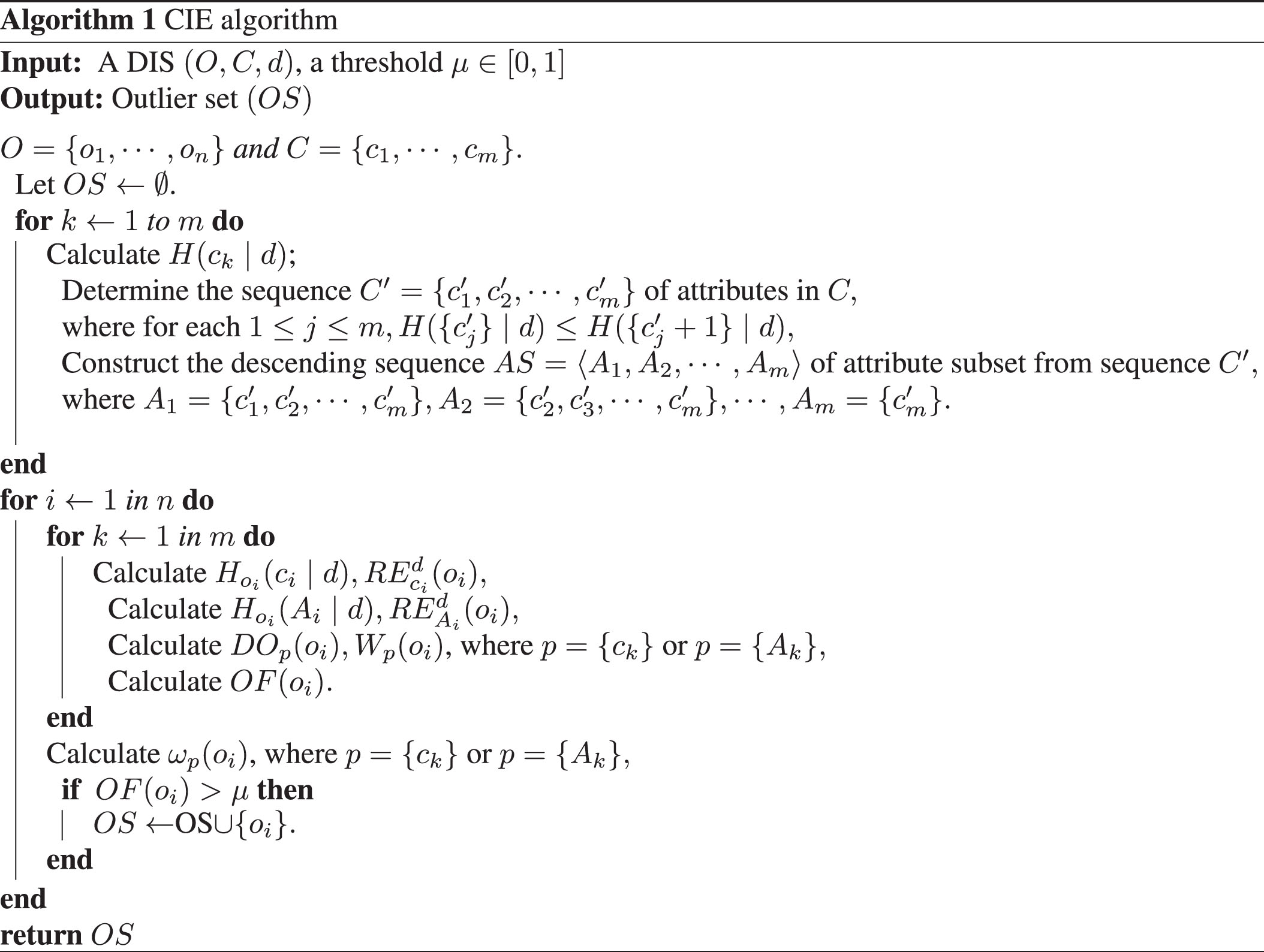
In this section, an outlier detection algorithm using conditional information entropy (denoted as CIE algorithm) is proposed.

6 Experiments

6.1 Experimental on twelve UCI Machine Learning data sets

To evaluate the effectiveness of the CIE algorithm, twelve data sets are selected from UCI for experiments [9]. On 12 data sets, we compare the performance of the CIE algorithm with Local Outlier Factor (LOF), k-Nearest Neighbor (KNN), Isolation Forest (Forest), One-Class Support Vector Machines (SVM) [33], Information Entropy-based (IE) [19], and Empirical-Cumulative-distribution-based Outlier Detection (ECOD) [43]. An overview of these seven algorithms used in this paper is shown in Table 1.

Most of public data sets are used for the evaluation of classification and clustering methods. For the evaluation of outlier detection, there are very few existing data sets. Accordingly, this article uses the downsampling method proposed in the document [5] to obtain some data sets for evaluating outlier detection methods. The method randomly downsamples a particular class to produce outliers while preserving all objects of the remaining classes to form a data set for evaluating outlier detection methods. In addition, for the missing values of data set, this article uses the maximum probability value method to complete the missing values, that is, the value of attribute with the highest frequency on other objects is used to fill the missing attribute values [38]. An overview of the data sets used in the paper is shown in Table 2.

Table 2

Seven concerned algorithms for outlier detection

Naming (Reference)	Meaning or strategy	Algorithm
LOF (Breunig et al., 2000)	Local Outlier Factor	Density Based
KNN (Ramaswamy et al., 2000)	K-nearest neighbor method	Distance Based
SVM (Scholkopf et al., 2001)	One-Class Support Vector Machines	Linear Model
Forest (Liu et al., 2008)	Isolation Forest Outlier Ensembles	Ensemble Based
IE (Jiang et al., 2010)	Information entropy based	Proximity Based
ECOD (Zheng Li et al.,2022)	Cumulative distribution based	Density Based
CIE	Conditional information entropy based	Proximity Based

In Table 2, the number of objects is between 132 and 4409, and the number of condictional features is between 8 and 36. The decision attribute is only one in every data set.

Fig. 2

Comparison by ROC curves and AUC values based on six methods.

The comparative experiments are conducted on a computer with the Intel (R) core (TM) i7-10700 processor plat-form, 2.90 GHz frequency, 8 G memory. The operating system is Windows 10. The experimental results are performed in Python3.8.

6.2 Evaluation metrics

In this paper, Precision (P), Recall (R), and Receiver Operating Characteristic (ROC) curves are used to evaluate the effectiveness of the proposed method [1]. The specific steps are as follows. In the outlier detection, most of the detection methods ultimately output the outlier factor of each object in O, and the larger the outlier factor of an object, the more likely it is the outlier. These objects can be arranged in descending order according to their outlier factor values. Given an order number t, objects with a sequence number greater than or equal to t are treated as outliers. If the given t is too small, it will cause the method to miss the true outliers. Conversely, too many objects are judged to be outliers, which leads to too excessive false positives. This trade-off can usually be measured by P and R. For a given t, OS (t)is a function of t [1]. It denotes the outlier set detected by the given t. OS ^O represents the true outlier set in the data set, and the P (t), R (t) are, respectively, calculated by $P\left(t\right)=\frac{\left|\mathit{OS}\right(t)\bigcap {\mathit{OS}}^O|}{\left|\mathit{OS}\right(t\left)\right|}\times 100\%$(16) $R\left(t\right)=\frac{\left|\mathit{OS}\right(t)\bigcap {\mathit{OS}}^O|}{\left|{\mathit{OS}}^O\right|}\times 100\%$(17) where P (t) denotes the proportion of true outliers detected under a given t. R (t) represents the proportion of true outliers detected under a given t in the total number of true outliers. The maximum possible value of P (t) and R (t) is 100%, and the minimum possible value is 0. Given the value of t, the larger the value of P (t) and R (t), the better outlier detection results. Obviously, whenP (t) and R (t) are given, the smaller the value of t, the better the detection effect. In addition, it can be proved that P (t) and R (t) are equal when t = |OS ^O | [38].

It is known that the ROC curves present a visual impression for the accuracy of diagnostic systems and display the tradeoffs between sensitivity and accuracy for various setting of the dicision criterion. And the Area Under the ROC curve(named AUC) gives expression to discrimination capacity for two classes of events. AUC analysis is widely recognized as the best method for measuring the quality of diagnostic information and diagnostic dicisions [1, 38].

The ROC curve is a curve with the false positive rate (FPR) as the abscissa and the true positive rate (TPR) as the ordinate.(FPR) and (TPR) are computed, respectively, as $\mathit{FPR}\left(t\right)=\frac{\left|\mathit{OS}\right(t)-{\mathit{OS}}^O|}{|O-{\mathit{OS}}^O|}\times 100\%$(18)

$\begin{array}{cc}\hfill & \mathit{TPR}\left(t\right)=R\left(t\right)=\frac{\left|\mathit{OS}\right(t)\bigcap {\mathit{OS}}^O|}{\left|{\mathit{OS}}^O\right|}\times 100\%\hfill \\ \hfill & \hfill \end{array}$(19) The ROC curve is used to compare the performance of different outlier detection algorithms. If the ROC curve of a detection algorithm is as close as possible to the upper left corner of the first quadrant, that is the AUC (area under the curve) value is larger, then the better its performance. In this section, the ROC curve and the corresponding AUC score are depicted, respectively, for each experiment.

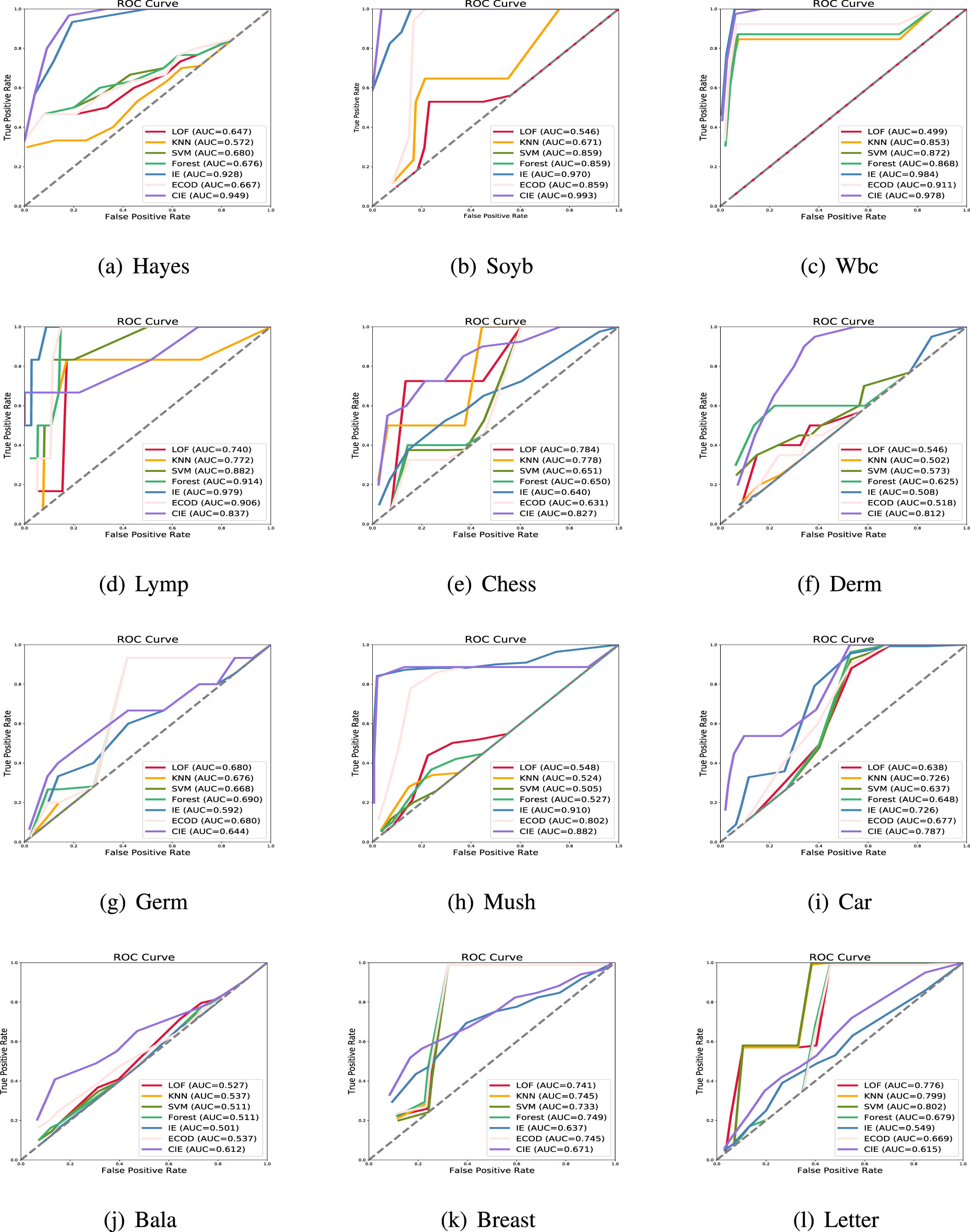
The ROC curves and the corresponding AUC values are described in Fig. 1, for investigated algorithms.

6.3 Experimental results and analyses

6.3.1 Comparison by P (t) and R (t)

Tables 3–5 show the experimental results for P (t) and R (t) on 12 data sets, respectively. They illustrate the results of the P (t) and R (t) change with t. From Table 3, it can be seen that the CIE algorithm achieves superior performance on Hayes, Soyb, Wbc data sets. The analyses are mainly carried out from the following aspects.

Table 3

Description of data and the details of data preprocessing

ID	Data set	Abbreviation	Preprocessing	Conditional feature	Outlier	Normal
1	Hayes-Roth	Hayes	Class "3" is treated as outlier,
		The decision attribute is ’Class’.	4	30	102
2	Soybean	Soyb	Classes "d-p-s-blight”,"c-nematode","h-injury”,
		and "2-4-d-injury” are treated as outliers,
		The decision attribute is ’classes’.	35	17	142
3	Wisconsin breast cancer	Wbc	202 "malignant” (outliers) and 14 "benign”,
		objects were removed, The decision attribute is ’Class’.	9	39	204
4	Lymphography	Lymp	Classes "1” and "4” are treated as outliers,
		The decision attribute is ’class’.	18	6	290
5	Chess	Chess	Downsampling class "2” to 40 objects,
		The decision attribute is ’Classes’.	36	40	346
6	Dermatology	Derm	Classes "pityriasis rubra pilaris” is treated as outlier,
		The decision attribute is the type of Disease.	33	20	444
7	German	Germ	Downsampling class "2” to 15 objects,
		The decision attribute is ’class’.	24	15	576
8	Mushroom	Mush	Downsampling class "+” to 221 objects,
		The decision attribute is ’class’.	22	201	699
9	Car evaluation	Car	Classes "good” and "vgood” are treated as outliers,
		The decision attribute is ’Class’.	6	134	1500
10	Balance scale	Bala	Class "B” is treated as outlier,
		The decision attribute is ’Class’.	4	49	1594
11	Breast cancer	Breast	Class "recurrence-events” is treated as outlier,
		The decision attribute is ’Class’.	8	85	1668
12	Letter	Letter	subsample data from 3 letters to form the normal,
		class and randomly concatenate pairs of them.	32	100	4208

Table 4

The comparison of experimental results about P (t) and R (t)\label t1

Data set	t	LOF		KNN		SVM		Forest		IE		ECOD		CIE
		P(t)	R(t)	P(t)	R(t)	P(t)	R(t)	P(t)	R(t)	P(t)	R(t)	P(t)	R(t)	P(t)	R(t)
Hayes	10	100.00	100.00	90.00	30.00	100.00	100.00	100.00	100.00	100.00	100.00	100.00	100.00	100.00	100.00
	20	70.00	46.67	50.00	33.33	70.00	46.67	70.00	46.67	85.00	56.67	70.00	46.67	85.00	56.67
	30	46.67	46.67	33.33	33.33	50.00	50.00	50.00	50.00	73.33	73.33	46.67	46.67	80.00	80.00
	40	37.50	50.00	30.00	40.00	42.50	56.67	45.00	60.00	70.00	93.33	42.50	56.67	72.50	96.67
	50	36.00	60.00	32.00	53.33	40.00	66.67	38.00	63.33	58.00	96.67	38.00	63.33	60.00	100.00
	60	33.33	66.67	31.67	63.33	35.00	70.00	35.00	70.00	50.00	100.00	33.33	66.67	50.00	100.00
	65	33.85	73.33	32.31	70.00	35.38	76.67	35.38	76.67	46.15	100.00	35.38	76.67	46.15	100.00
	70	32.86	76.67	30.00	70.00	34.29	80.00	32.86	76.67	42.86	100.00	34.29	80.00	42.86	100.00
	80	31.25	83.33	26.25	70.00	31.25	83.33	28.75	76.67	37.50	100.00	30.00	80.00	37.50	100.00
	90	27.78	83.33	23.33	70.00	27.78	83.33	25.56	76.67	33.33	100.00	27.78	83.33	33.33	100.00
	Average	44.64	67.83	37.65	52.63	46.34	70.50	45.80	68.90	59.28	91.00	45.51	69.17	60.40	92.33
Soyb	10	0.00	0.00	20.00	11.76	20.00	11.76	20.00	11.76	100.00	100.00	20.00	11.76	100.00	100.00
	20	10.00	11.76	20.00	23.53	30.00	35.29	30.00	35.29	70.00	82.35	30.00	35.29	85.00	100.00
	25	20.00	29.41	36.00	52.94	44.00	64.71	44.00	64.71	60.00	88.24	44.00	64.71	68.00	100.00
	30	30.00	52.94	36.67	64.71	53.33	94.12	53.33	94.12	56.67	100.00	53.33	94.12	56.67	100.00
	35	25.71	52.94	31.43	64.71	48.57	100.00	48.57	100.00	48.57	100.00	48.57	100.00	48.57	100.00
	40	22.50	52.94	27.50	64.71	42.50	100.00	42.50	100.00	42.50	100.00	42.50	100.00	42.50	100.00
	45	20.00	52.94	24.44	64.71	37.78	100.00	37.78	100.00	37.78	100.00	37.78	100.00	37.78	100.00
	50	18.00	52.94	22.00	64.71	34.00	100.00	34.00	100.00	34.00	100.00	34.00	100.00	34.00	100.00
	60	15.00	52.94	18.33	64.71	28.33	100.00	28.33	100.00	28.33	100.00	28.33	100.00	28.33	100.00
	Average	17.72	39.22	26.03	52.14	37.26	77.20	37.26	77.20	52.74	95.50	37.26	77.20	55.29	98.77
Wbc	20	5.00	2.56	65.00	33.33	65.00	33.33	60.00	30.77	90.00	46.15	65.00	33.33	85.00	43.59
	39	7.69	7.69	66.67	66.67	66.67	66.67	61.54	61.54	76.92	76.92	66.67	66.67	74.36	74.36
	60	15.00	23.08	55.00	84.62	56.67	87.18	56.67	87.18	65.00	100.00	60.00	92.31	63.33	97.44
	100	10.00	25.64	33.00	84.62	34.00	87.18	34.00	87.18	39.00	100.00	36.00	92.31	39.00	100.00
	120	8.33	25.64	27.50	84.62	28.33	87.18	28.33	87.18	32.50	100.00	30.00	92.31	32.50	100.00
	150	6.67	25.64	22.00	84.62	22.67	87.18	22.67	87.18	26.00	100.00	24.00	92.31	26.00	100.00
	200	5.00	25.64	16.50	84.62	17.00	87.18	17.00	87.18	19.50	100.00	18.00	92.31	19.50	100.00
	250	4.00	25.64	13.20	84.62	13.60	87.18	13.60	87.18	15.60	100.00	14.40	92.31	15.60	100.00
	300	3.33	25.64	11.00	84.62	11.33	87.18	11.33	87.18	13.00	100.00	12.00	92.31	13.00	100.00
	Average	7.18	20.48	34.29	75.88	34.89	77.84	33.76	76.99	41.78	90.22	36.08	81.77	40.76	89.36
Lymp	3	33.33	16.67	0.00	0.00	66.67	33.33	66.67	33.33	100.00	100.00	33.33	16.67	100.00	100.00
	4	25.00	16.67	25.00	16.67	50.00	33.33	50.00	33.33	75.00	50.00	50.00	33.33	100.00	100.00
	5	20.00	16.67	40.00	33.33	40.00	33.33	60.00	50.00	80.00	66.67	40.00	33.33	80.00	66.67
	6	16.67	16.67	50.00	50.00	50.00	50.00	50.00	50.00	83.33	83.33	33.33	33.33	66.67	66.67
	7	14.29	16.67	42.86	50.00	42.86	50.00	42.86	50.00	71.43	83.33	42.86	50.00	57.14	66.67
	9	33.33	50.00	44.44	66.67	55.56	83.33	44.44	66.67	66.67	100.00	55.56	83.33	44.44	66.67
	11	45.45	83.33	45.45	83.33	45.45	83.33	54.55	100.00	54.55	100.00	54.55	100.00	36.36	66.67
	12	41.67	83.33	41.67	83.33	41.67	83.33	50.00	100.00	50.00	100.00	50.00	100.00	33.33	66.67
	23	21.74	83.33	21.74	83.33	26.09	100.00	26.09	100.00	26.09	100.00	26.09	100.00	21.74	83.33
	30	16.67	83.33	16.67	83.33	20.00	100.00	20.00	100.00	20.00	100.00	20.00	100.00	20.00	100.00
	Average	26.64	45.83	32.61	54.17	43.62	64.00	46.25	67.33	62.50	82.33	40.36	64.00	55.77	77.35

Table 5

The comparison of experimental results about P (t) and R (t)

Data set	t	LOF		KNN		SVM		Forest		IE		ECOD		CIE
		P(t)	R(t)	P(t)	R(t)	P(t)	R(t)	P(t)	R(t)	P(t)	R(t)	P(t)	R(t)	P(t)	R(t)
Car	50	0.00	0.00	14.00	5.22	0.00	0.00	6.00	2.24	14.00	5.22	0.00	0.00	44.00	16.42
	80	0.00	0.00	12.50	7.46	0.00	0.00	3.75	2.24	12.50	7.46	7.50	4.48	47.50	28.36
	100	0.00	0.00	12.00	8.96	1.00	0.75	3.00	2.24	12.00	8.96	6.00	4.48	47.00	35.07
	134	0.00	0.00	16.42	16.42	1.49	1.49	3.73	3.73	16.42	16.42	5.97	5.97	44.78	44.78
	200	2.00	2.99	22.00	32.84	3.00	4.48	6.50	9.70	22.00	32.84	10.5	15.67	36.00	53.73
	400	10.25	30.60	12.00	35.82	7.75	23.13	8.75	26.12	12.00	35.82	13.50	40.30	18.00	53.73
	600	11.00	49.25	17.67	79.10	10.67	47.76	11.00	49.25	17.67	79.10	13.33	59.70	15.00	67.16
	800	14.75	88.06	16.00	95.52	15.50	92.54	16.12	96.27	16.00	95.52	15.12	90.30	16.75	100.00
	1000	13.3	99.25	13.30	99.25	13.30	99.25	13.40	100.00	13.30	99.25	13.40	100.00	13.40	100.00
	1200	11.08	99.25	11.08	99.25	11.08	99.25	11.17	100.00	11.08	99.25	11.17	100.00	11.17	100.00
	1400	9.50	99.25	9.50	99.25	9.50	99.25	9.57	100.00	9.50	99.25	9.57	100.00	9.57	100.00
	Average	6.46	41.78	14.14	51.83	6.58	41.72	8.37	43.88	14.14	51.83	9.56	46.53	27.48	62.74
Bala	49	10.20	10.20	16.33	16.33	10.20	10.20	10.20	10.20	6.12	6.12	16.33	16.33	20.41	20.41
	80	8.75	14.29	12.50	20.41	8.75	14.29	10.00	16.33	7.50	12.24	12.50	20.41	20.00	32.65
	100	9.00	18.37	12.00	24.49	9.00	18.37	9.00	18.37	8.00	16.33	12.00	24.49	20.00	40.82
	200	9.00	36.73	9.50	38.78	8.50	34.69	8.00	32.65	7.50	30.61	9.50	38.78	12.00	48.98
	250	8.00	40.82	9.20	46.94	7.60	38.78	7.20	36.73	7.60	38.78	9.20	46.94	10.80	55.10
	300	8.33	51.02	8.67	53.06	7.67	46.94	7.67	46.94	7.33	44.90	8.67	53.06	10.67	65.31
	400	8.75	71.43	8.00	65.31	8.25	67.35	8.25	67.35	8.25	67.35	8.00	65.31	9.00	73.47
	450	8.67	79.59	8.22	75.51	8.22	75.51	8.44	77.55	7.78	71.43	8.22	75.51	8.44	77.55
	500	8.00	81.63	7.80	79.59	7.80	79.59	7.80	79.59	7.80	79.59	7.80	79.59	8.20	83.67
	550	7.64	85.71	7.82	87.76	7.45	83.67	7.64	85.71	7.82	87.76	7.82	87.76	7.64	85.71
	600	7.67	93.88	7.67	93.88	7.50	91.84	7.67	93.88	7.67	93.88	7.67	93.88	7.83	95.92
	Average	8.48	52.29	9.73	53.96	8.21	50.27	8.29	50.62	7.52	49.14	9.73	53.96	12.21	61.00
Breast	50	38.00	22.35	36.00	21.18	34.00	20.00	38.00	22.35	50.00	29.41	40.00	23.53	56.00	32.94
	85	25.88	25.88	28.24	28.24	23.53	23.53	29.41	29.41	43.53	43.53	27.06	27.06	51.76	51.76
	100	37.00	43.53	39.00	45.88	35.00	41.18	40.00	47.06	40.00	47.06	38.00	44.71	48.00	56.47
	150	56.00	98.82	56.00	98.82	56.00	98.82	56.00	98.82	39.33	69.41	56.00	98.82	38.00	67.06
	180	46.67	98.82	46.67	98.82	46.67	98.82	46.67	98.82	35.56	75.29	46.67	98.82	35.56	75.29
	200	42.00	98.82	42.00	98.82	42.00	98.82	42.00	98.82	33.00	77.65	42.00	98.82	35.00	82.35
	220	38.18	98.82	38.18	98.82	38.18	98.82	38.18	98.82	31.82	82.35	38.18	98.82	32.73	84.71
	240	35.00	98.82	35.00	98.82	35.00	98.82	35.00	98.82	30.00	84.71	35.00	98.82	31.25	88.24
	260	32.31	98.82	32.31	98.82	32.31	98.82	32.31	98.82	30.00	91.76	32.31	98.82	30.77	94.12
	280	30.00	98.82	30.00	98.82	30.00	98.82	30.00	98.82	29.64	97.65	30.00	98.82	29.29	96.47
	290	29.72	100.00	29.72	100.00	29.72	100.00	29.72	100.00	29.72	100.00	29.72	100.00	29.72	100.00
	Average	37.10	79.50	37.31	79.82	36.34	78.85	37.69	80.14	35.45	71.80	37.48	79.82	37.56	74.58
Letter	50	0.00	0.00	4.00	2.00	2.00	1.00	2.00	1.00	10.00	5.00	0.00	0.00	12.00	6.00
	100	22.00	22.00	4.00	4.00	2.00	2.00	1.00	1.00	8.00	8.00	0.00	0.00	12.00	12.00
	200	28.50	57.00	28.50	57.00	29.00	58.00	8.50	17.00	8.50	17.00	5.50	11.00	11.50	23.00
	300	19.00	57.00	19.00	57.00	19.33	58.00	5.67	17.00	8.33	25.00	3.67	11.00	11.67	35.00
	400	14.25	57.00	14.25	57.00	14.50	58.00	4.25	17.00	9.75	39.00	2.75	11.00	10.50	42.00
	500	11.40	57.00	11.40	57.00	11.60	58.00	3.40	17.00	8.80	44.00	2.20	11.00	9.40	47.00
	600	9.67	58.00	16.50	99.00	16.67	100.00	11.33	68.00	8.17	49.00	10.83	65.00	8.83	53.00
	700	14.29	100.00	14.29	100.00	14.29	100.00	14.29	100.00	7.57	53.00	14.14	99.00	9.00	63.00
	800	12.50	100.00	12.50	100.00	12.50	100.00	12.50	100.00	7.88	63.00	12.38	99.00	9.00	72.00
	1000	10.00	100.00	10.00	100.00	10.00	100.00	10.00	100.00	7.40	74.00	9.90	99.00	8.00	80.00
	1200	8.33	100.00	8.33	100.00	8.33	100.00	8.33	100.00	7.17	86.00	8.25	99.00	7.92	95.00
	Average	13.56	63.54	12.91	65.81	12.68	65.99	7.32	48.08	8.26	41.39	6.26	45.09	9.92	47.23

Table 6

The comparison of experimental results about P (t) and R (t)

Data set	t	LOF		KNN		SVM		Forest		IE		ECOD		CIE
		P(t)	R(t)	P(t)	R(t)	P(t)	R(t)	P(t)	R(t)	P(t)	R(t)	P(t)	R(t)	P(t)	R(t)
Chess	40	2.50	2.50	22.50	22.50	2.50	2.50	2.50	2.50	10.00	10.00	2.50	2.50	20.00	20.00
	100	1.00	2.50	20.00	50.00	1.00	2.50	1.00	2.50	9.00	22.50	1.00	2.50	22.00	55.00
	200	14.50	72.50	10.00	50.00	7.50	37.50	8.00	40.00	7.50	37.50	6.50	32.50	12.00	60.00
	300	9.67	72.50	6.67	50.00	5.00	37.50	5.33	40.00	6.00	45.00	4.33	32.50	9.67	72.50
	400	7.25	72.50	5.00	50.00	3.75	37.50	4.00	40.00	5.25	52.50	3.25	32.50	7.25	72.50
	500	5.80	72.50	4.00	50.00	3.00	37.50	3.20	40.00	4.60	57.50	2.60	32.50	6.80	85.00
	600	4.83	72.50	6.67	100.00	3.50	52.50	3.00	45.00	4.33	65.00	3.00	45.00	6.00	90.00
	800	5.00	100.00	5.00	100.00	5.00	100.00	5.00	100.00	3.62	72.50	5.00	100.00	4.62	92.50
	1000	4.00	100.00	4.00	100.00	4.00	100.00	4.00	100.00	3.40	85.00	4.00	100.00	4.00	100.00
	1200	3.33	100.00	3.33	100.00	3.33	100.00	3.33	100.00	3.25	97.50	3.33	100.00	3.33	100.00
	Average	5.75	65.75	8.68	66.25	3.82	49.75	3.90	50.00	5.66	53.54	3.52	47.00	9.53	73.75
Derm	20	5.00	5.00	10.00	10.00	25.00	25.00	30.00	30.00	10.00	10.00	5.00	5.00	20.00	20.00
	40	17.50	35.00	10.00	20.00	17.50	35.00	25.00	50.00	7.50	15.00	10.00	20.00	22.50	45.00
	60	13.33	40.00	8.33	25.00	13.33	40.00	20.00	60.00	5.00	15.00	11.67	35.00	21.67	65.00
	80	10.00	40.00	7.50	30.00	11.25	45.00	15.00	60.00	5.00	20.00	8.75	35.00	20.00	80.00
	90	11.11	50.00	6.67	30.00	10.00	45.00	13.33	60.00	4.44	20.00	10.00	45.00	20.00	90.00
	100	10.00	50.00	6.00	30.00	10.00	50.00	12.00	60.00	4.00	20.00	9.00	45.00	19.00	95.00
	135	7.41	50.00	7.41	50.00	8.89	60.00	8.89	60.00	7.41	50.00	6.67	45.00	14.81	100.00
	140	7.14	50.00	7.14	50.00	10.00	70.00	8.57	60.00	7.86	55.00	6.43	45.00	14.29	100.00
	180	6.67	60.00	7.22	65.00	7.78	70.00	8.33	75.00	7.78	70.00	7.78	70.00	11.11	100.00
	Average	9.71	41.49	7.72	33.66	12.54	48.03	15.58	56.31	6.46	29.71	8.27	37.50	21.60	59.33
Germ	15	0.00	0.00	0.00	0.00	0.00	0.00	0.00	0.00	0.00	0.00	0.00	0.00	6.67	6.67
	70	4.29	20.00	2.86	13.33	1.43	6.67	5.71	26.67	4.29	20.00	4.29	20.00	7.14	33.33
	100	3.00	20.00	3.00	20.00	2.00	13.33	4.00	26.67	5.00	33.33	3.00	20.00	6.00	40.00
	200	1.50	20.00	1.50	20.00	1.00	13.33	2.00	26.67	3.00	40.00	1.50	20.00	4.00	53.33
	300	4.67	93.33	4.67	93.33	4.67	93.33	4.67	93.33	3.00	60.00	4.67	93.33	3.33	66.67
	400	3.50	93.33	3.50	93.33	3.50	93.33	3.50	93.33	2.50	66.67	3.50	93.33	2.5	66.67
	500	2.80	93.33	2.80	93.33	2.80	93.33	2.80	93.33	2.40	80.00	2.80	93.33	2.40	80.00
	550	2.55	93.33	2.55	93.33	2.55	93.33	2.55	93.33	2.18	80.00	2.55	93.33	2.18	80.00
	600	2.33	93.33	2.33	93.33	2.33	93.33	2.33	93.33	2.00	80.00	2.33	93.33	2.33	93.33
	650	2.15	93.33	2.15	93.33	2.15	93.33	2.15	93.33	2.00	86.67	2.15	93.33	2.15	93.33
	700	2.00	93.33	2.00	93.33	2.00	93.33	2.00	93.33	2.14	100.00	2.00	93.33	2.14	100.00
	Average	2.60	64.08	2.47	63.47	2.20	61.65	2.87	65.90	2.57	57.97	2.60	64.08	3.70	65.03
Mush	50	16.00	3.62	28.00	6.33	24.00	5.43	26.00	5.88	100.00	100.00	52.00	11.76	88.00	19.91
	100	17.00	7.69	30.00	13.57	26.00	11.76	22.00	9.95	100.00	100.00	50.00	22.62	94.00	42.53
	201	23.38	21.27	30.85	28.05	21.89	19.91	25.87	23.53	92.54	84.16	52.74	47.96	92.04	83.71
	300	32.33	43.89	25.00	33.94	18.67	25.34	27.00	36.65	64.33	87.33	57.33	77.83	65.33	88.69
	400	27.75	50.23	19.25	34.84	17.00	30.77	23.25	42.08	48.75	88.24	47.50	85.97	49.00	88.69
	500	23.00	52.04	15.80	35.75	14.40	32.58	19.20	43.44	39.00	88.24	39.20	88.69	39.20	88.69
	600	19.17	52.04	14.00	38.01	12.33	33.48	16.17	43.89	33.17	90.05	32.67	88.69	32.67	88.69
	700	16.43	52.04	12.29	38.91	10.57	33.48	14.29	45.25	28.71	90.95	28.00	88.69	28.00	88.69
	800	14.62	52.94	10.75	38.91	9.50	34.39	12.62	45.70	26.62	96.38	24.50	88.69	24.50	88.69
	900	13.00	52.94	9.67	39.37	8.89	36.20	11.33	46.15	24.11	98.19	21.78	88.69	21.78	88.69
	1000	11.70	52.94	8.70	39.37	8.00	36.20	10.20	46.15	21.70	98.19	19.60	88.69	19.70	89.14
	Average	19.39	39.71	18.50	31.23	15.50	26.93	18.82	34.95	52.45	92.07	38.50	70.02	50.22	77.09

(1) Given t = |OS ^o |, the CIE algorithm has a larger P (t). For example, for the Hayes data set, the CIE algorithm’s P (t) is 80.00%. However, for LOF, KNN, SVM, Forest, IE, and ECOD algorithms, their P (t) are 46.67%, 33.33%, 50.00%, 50.00%, 73.33%, and 46.67%, respectively. The P (t) of the CIE algorithm is larger than that of other algorithms. On Soyb, Chess, Car, Bala, Derm and Wbc data sets, the CIE algorithm’s P (t) is greater than or equal to that of other algorithms. For the Lymp, Breast, Germ, Mush and Letter data sets, the P (t) of the CIE algorithm is slightly smaller than that of the IE algorithm, but greater than other algorithms. For the Chess, Derm and Cmc data sets, the P (t) of the CIE algorithm is smaller than or equal to other algorithms.

(2) In terms of R (t), the CIE algorithm achieves maximum values in most data sets for given t = |OS ^o |. For example, in the Wbc data set, the CIE algorithm’s R (t) is 100.00% at first time, but, for LOF, KNN, LOF, SVM, Forest, IE, and ECOD algorithms, their R (t) are 25.64%, 84.62%, 87.18%, 87.18%, 100% and 92.31%, respectively. For Hayes, Soyb, Mush Bala, Car and Wbc data sets, the CIE algorithm’s R (t) is greater than other algorithms. On the Chess, Lymp, Breat, Derm, Germ and Letter data sets, the R (t) of the CIE algorithm is slightly smaller than that of the other’s algorithm.

(3) For the average of P (t) and R (t), the CIE algorithm achieves maximum values on the Hayes, Soyb, Wbc, Derm, Germ, Chess, Car, and Bala data sets. For example, the average P (t) and R (t) of the CIE algorithm on the Hayes data set are 60.40% and 92.33%, respectively, which is obviously larger than other algorithms. For the Lymp, Wbc and Mush data sets, the average P (t) and R (t) of the CIE algorithm are slightly smaller than that of the IE algorithm, but greater than other algorithms. However, for the Breast and Letter data sets, the average P (t) and R (t) of the CIE algorithm are slightly smaller than or equal to that of other algorithms.

6.4 Comparison by ROC curves and AUC values

From Fig. 1, the experimental result reveals that CIE algorithm attains the highist AUC value for Hayes, Soyb, Chess, Derm, Car, Bala and Wbc data sets. For example, in the Hayes data set, the AUC value of CIE algorithm is 0.949, however, for LOF, KNN, SVM, Forest, IE and ECOD algorithms, their AUC values are 0.647, 0.572, 0.680, 0.676, 0.928 and 0.667, respectively. For the Mush data set, the AUC score of the CIE algorithm is smaller than that of the IE algorithm, but higher than the others algorithms. Only for the Lymp, Germ, Breast and Letter data sets, the result of AUC from CIE algorithm are slightly smaller than or equal to that of other algorithms.

7 Conclusion

Based on RST and information entropy, this paper has proposed a supervised method for outlier detection in a DIS. In terms of this method, we have designed the corresponding algorithm, and carried out experiments to compare with some existing outlier detection algorithms. Experimental results have demonstrated that the designed algorithm is effective. A supervised method for outlier detection using conditional information entropy has not been studied before. This is the innovation of this paper. The existing state-of-the-art outlier detection algorithms mainly are unsupervised because they are only dealt with unlabeled data. When sufficient labeled data are available and these algorithms are used in a DIS, this means that the decision attribute is discarded and then leads to information loss. The proposed outlier detection algorithm fully utilizes the decision information. This reflects the main differences or importance between the proposed algorithm and other state-of-the-art algorithms. The proposed work has the limitation, i.e., it can it can only detect the outliers of categorical data. We wish that the proposed work could improve the accuracy of deep learning detection methods. In future work, we will extend the proposed work to mixed data and fuzzy information entropy based outlier detection.