A coarse-to-fine unsupervised domain adaptation method based on metric learning

Abstract

Domain adaptation solves the challenge of inadequate labeled samples in the target domain by leveraging the knowledge learned from the labeled source domain. Most existing approaches aim to reduce the domain shift by performing some coarse alignments such as domain-wise alignment and class-wise alignment. To circumvent the limitation, we propose a coarse-to-fine unsupervised domain adaptation method based on metric learning, which can fully utilize more geometric structure and sample-wise information to obtain a finer alignment. The main advantages of our approach lie in four aspects: (1) it employs a structure-preserving algorithm to automatically select the optimal subspace dimension on the Grassmannian manifold; (2) based on coarse distribution alignment using maximum mean discrepancy, it utilizes the smooth triplet loss to leverage the supervision information of samples to improve the discrimination of data; (3) it introduces structure regularization to preserve the geometry of samples; (4) it designs a graph-based sample reweighting method to adjust the weight of each source domain sample in the cross-domain task. Extensive experiments on several public datasets demonstrate that our method achieves remarkable superiority over several competitive methods (more than 1.5% improvement of the average classification accuracy over the best baseline).

1 Introduction

Many real-world tasks suffer from insufficient labeled samples and discrepant distributions of the training and testing data [1]. To address these challenges, domain adaptation utilizes a related and adequately annotated domain (source domain) to assist the task of the current domain (target domain) by reducing the distribution discrepancy between the two domains. This approach has shown remarkable performance in practical applications such as object detection [2–4], natural language processing [5–8], medical image analysis [9–13] and image classification [14–18]. The domain adaptation methods for reducing the discrepancy between two domains can be roughly categorized into two types [19]: instance-based and feature-based methods. Instance-based domain adaptation methods reweight the source domain samples through weight generation rules, thereby the weighted source domain distribution becomes closer to that of the target domain. Some methods [20–22] estimate the distribution ratio between the two domains as the weight of the source domain sample. However, relying on the estimation of probability distribution limits the performance of these methods.

On the other hand, feature-based domain adaptation methods map the source and target domain data into a shared space where the domain shift is small. They align the marginal distribution [14], conditional distribution or both [16, 23] by using a proper distribution distance measure such as maximum mean discrepancy (MMD) [24]. Unfortunately, most feature-based algorithms focus on coarse domain-wise alignment and class-wise alignment, which is far from enough.

To achieve finer alignment, metric learning-based domain adaptation approaches [25–28] learn a suitable metric matrix to address the scarcity of labeled data and distribution disparity by leveraging sample information. Such a metric matrix brings similar samples closer while pushing apart dissimilar ones, thereby enhancing the classification accuracy. Nevertheless, the subspace dimension in these methods is a hyper-parameter and is not guaranteed to be optimal. Moreover, most of these methods only reduce the distribution difference from a statistical perspective, failing to preserve the geometry of the data very well. Without structure constraints, the original data structure will be destroyed.

In this paper, to tackle the aforesaid deficiencies, we propose a metric learning-based coarse-to-fine unsupervised domain adaptation method. Specifically, subspace learning can be treated as an inverse problem on the Grassmannian manifold, searching for the optimal subspace dimension by a structure-preserving algorithm. In this way, the dimension of the subspace no longer needs to be artificially set before the experiment. Meanwhile, we reduce the distribution discrepancy and improve the separability between different classes to get coarse alignment. For a finer alignment, we improve the discrimination of data by using the smooth triplet loss and preserve the geometry of data by introducing structure regularization. Finally, a graph-based sample reweighting method is utilized to adjust the weights of source domain samples in the cross-domain task.

Our contributions can be summarized as follows:

We adopt a structure-preserving algorithm to automatically select the optimal subspace dimension on the Grassmannian manifold.

We introduce the smooth triplet loss and structure regularization into domain adaptation and propose a coarse-to-fine unsupervised domain adaptation model.

We design a graph-based sample reweighting method to pick out the most task-relevant source domain samples.

Extensive quantitative evaluations on benchmark datasets validate that our method performs an outstanding improvement against previous methods.

The remainder of this article is organized as follows. In the following section, we outline the related work. Section 3 describes our novel domain adaptation model in detail. Section 4 presents the optimization process of our algorithm. An extensive experimental study is provided in Section 5. Finally, we conclude this article in Section 6.

2 Related work

2.1 Domain adaptation

Domain adaptation aims to reduce the distribution divergence by using different strategies. According to [19], we broadly divide existing domain adaptation approaches into two classes: instance-based and feature-based domain adaptation.

Instance-based domain adaptation methods reduce the domain shift via reweighting source instances according to their correlations with target instances. Transfer joint matching (TJM) [15] reweights the instances by minimizing the ℓ_2,1-norm structured sparsity penalty. Later, metric transfer learning framework (MTLF) [22] learns the weights of source instances by minimizing the Kullback-Leibler divergence (KL-divergence) between the weighted source data distribution and the target data distribution. Recently, unsupervised domain adaptation based on adaptive local manifold learning (UDA-ALML) [29] uses the reconstruction coefficient matrix as the weight matrix when reconstructing the target samples. Moreover, transfer independently together (TIT) [30] uses the graph-based method to compute the intra-domain weights of source domain samples. Differently, intra-class weights are calculated in our method.

In recent years, feature-based domain adaptation methods have been extensively developed. Transfer component analysis (TCA) [14] minimizes the marginal distribution discrepancy between domains by using MMD distance. Based on TCA, joint distribution adaptation (JDA) [23] further considers the conditional distribution difference. Later, balanced distribution adaptation (BDA) [16] and manifold embedded distribution alignment (MEDA) [31] introduce a weight parameter to measure the influences of conditional and marginal distributions. Then, Li et al. [32] introduced a manifold regularization method to keep the neighbor relations of the data based on BDA. Joint probability domain adaptation (JPDA) [17] replaces the frequently used joint MMD with joint probability MMD to simultaneously increase the transfer performance and discriminative ability. Subsequently, Lie group manifold analysis (LGMA) [33] combines Lie group theory, weighted distribution alignment and manifold alignment to minimize the domain mismatch. Discriminative invariant alignment (DIA) [34] introduces the maximum margin criterion to improve the discriminant ability and encodes the Laplacian embedding technique to preserve the geometrical consistency of the target domain. Moreover, Yang et al. [35] introduced a class-wise sparsity regularization to maintain the row-sparsity consistency of samples from the same class. Recently, discriminative manifold distribution alignment (DMDA) [36] uses the Hilbert-Schmidt independence criterion to keep the source label information. Unlike these methods, we introduce metric learning into domain adaptation to employ sample-wise information.

2.2 Metric learning-based domain adaptation

Metric learning-based domain adaptation methods take advantage of both domain adaptation and metric learning, and thus have received tremendous attention recently. Decomposition-based transfer distance metric learning (DTDML) [25] argues that the target metric consists of the decomposition of source metrics. Then, robust transfer metric learning (RTML) [26] seeks a more robust transfer low-rank metric by designing a marginalized denoising scheme. Metric transfer learning framework (MTLF) [22] reweights source instances with the Mahalanobis distance. Later, unsupervised transfer metric learning (UTML) [27] further employs the target discriminative information. Subsequently, to achieve better performance, Kerdoncuff et al. [37] encoded optimal transport and metric learning into domain adaptation. Recently, geometric mean transfer learning (GMTL) [28] combines transfer learning and geometric mean metric learning to improve the discriminability of learned features. In contrast to these methods, we introduce a structure preservation term to retain the geometric consistency of samples and adopt a manifold dimension reduction method to select the optimal subspace dimension automatically.

3 Proposed method

Firstly, we state the problem of domain adaptation. Let ${\mathcal{D}}_{\mathcal{s}}=\left\{\right({\mathcal{x}}_{\mathcal{i}},{\mathcal{y}}_{\mathcal{i}}\left)\right|\mathcal{i}=1,\dots ,{\mathcal{n}}_{\mathcal{s}}\}$ denote the labeled source domain and ${\mathcal{D}}_{\mathcal{t}}=\left\{{\mathcal{x}}_{\mathcal{j}}\right|\mathcal{j}={\mathcal{n}}_{\mathcal{s}}+1,\dots ,{\mathcal{n}}_{\mathcal{s}}+{\mathcal{n}}_{\mathcal{t}}\}$ denote the unlabeled target domain, where x_i , ${\mathit{x}}_{\mathit{j}}\in {ℝ}^d$ , d is the dimension of data, y _i  ∈ {1, …, n _c } is the label of sample x_i , n _c is the number of classes, n _s and n _t indicate the numbers of source and target samples, respectively. Assume that ${\mathcal{D}}_{\mathcal{s}}$ and ${\mathcal{D}}_{\mathcal{t}}$ have the same label space. $X_s\in {ℝ}^{d\times n_s}$ and $X_t\in {ℝ}^{d\times n_t}$ indicate the source and target data matrices, respectively. Our goal is to learn a cross-domain low-rank metric M which can assist the target task by utilizing labeled and relevant source data. With the metric M, the squared distance between two samples x _i and x _j is defined as $d_{\mathit{ij}}^2=({\mathit{x}}_i-{\mathit{x}}_j{)}^{\top }M({\mathit{x}}_i-{\mathit{x}}_j)$ . Fig. 1 illustrates the overall framework of the proposed method.

Fig. 1

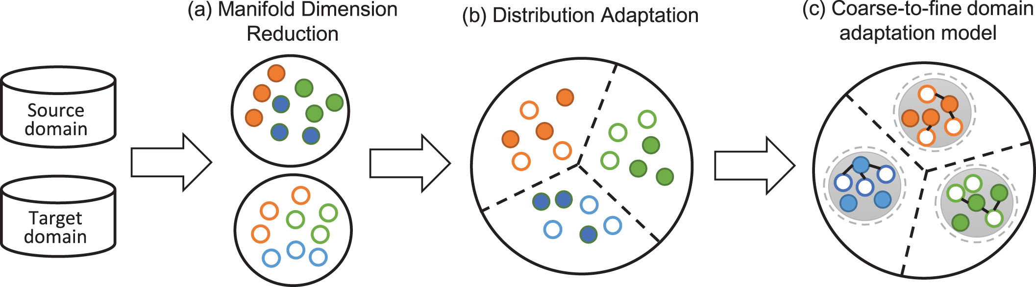
Illustration of the proposed method. (a) Manifold dimension reduction is used to map the source and target domains into the optimal subspace. (b) We reduce the domain discrepancy and improve the divisibility of data between different classes by distribution adaptation. (c) By the coarse-to-fine domain adaptation model, similar samples become closer while dissimilar samples become farther. Different colors represent different classes.

3.1 Manifold dimension reduction

In many existing methods, samples of source and target domains are mapped into a low-dimensional domain-invariant subspace. However, the dimension of the subspace is a hyper-parameter which is artificially set before the experiment. In this paper, a manifold dimension reduction method is adopted to automatically select the optimal subspace dimension.

Motivated by [38], we regard all subspaces as points on a Grassmannian manifold and solve the subspace learning problem as an inverse problem on the Grassmannian manifold. Specifically, all subspaces can be represented uniformly by using the method of the rotation group SO (d) action. We denote the i ^th orthogonal basis as e _i  = (0, …, 1, …, 0) ^⊤. Let B _r  = span { e ₁, …, e _r } be the standard r-dimensional subspace. Then there exists a rotation R ∈ SO (d) such that for any r-dimensional subspace $𝕊\in \mathit{Gr}(d,r)$ , we have $𝕊={\mathit{RB}}_r$ . Therefore, the Grassmannian manifold can be expressed as Gr (d, r) = {RB _r |R ∈ SO (d)}.

A step further, let P _r  = [ e ₁, …, e _r ] ^⊤ be the projection matrix from Euclidean space ${ℝ}^d$ to B _r , we can represent the transformation process of ${ℝ}^d$ to subspace $𝕊$ as ${ℝ}^d\stackrel{P_r}{⟶}{B}_r\stackrel{R}{⟶}𝕊.$

Thus, in the learned subspace, the corresponding sample of the original sample x _i can be expressed as $P_r^{\top }{R}^{\top }{\mathit{x}}_i$ .

3.2 Distribution adaptation

Although the features are more favorable for task performance after subspace learning, the problem of the distribution gap still exists. We learn a robust cross-domain metric M to narrow the difference in marginal and conditional distributions between domains using MMD distance. Under the action of rotation matrix R and projection matrix P _r , the forms of marginal distribution alignment and conditional distribution alignment are $\begin{array}{cc}\hfill \underset{M}{min}& \left(P_r^{\top }{R}^{\top }\right({\mu }_s-{\mu }_t\left){)}^{\top }M\right(P_r^{\top }{R}^{\top }({\mu }_s-{\mu }_t))\hfill \\ \hfill =\underset{M}{min}& \mathrm{tr}\left(\Phi {\mathit{RP}}_r{\mathit{MP}}_r^{\top }{R}^{\top }\right),\hfill \end{array}$(1) and $\begin{array}{cc}\hfill \underset{M}{min}& \sum _{c=1}^{n_c}\left(P_r^{\top }{R}^{\top }\right({\mu }_s^c-{\mu }_t^c\left){)}^{\top }M\right(P_r^{\top }{R}^{\top }({\mu }_s^c-{\mu }_t^c))\hfill \\ \hfill =\underset{M}{min}& \sum _{c=1}^{n_c}\mathrm{tr}\left({\Phi }^c{\mathit{RP}}_r{\mathit{MP}}_r^{\top }{R}^{\top }\right),\hfill \end{array}$(2) where $M\in {𝕊}_d^{+}$ , ${𝕊}_d^{+}$ is a d-dimensional positive definite matrix group. ${\mu }_s=\left({\sum }_{i=1}^{n_s}{\mathit{x}}_i\right)/n_s$ is the center of the source domain, and ${\mu }_t=\left({\sum }_{i=n_s+1}^{n_s+n_t}{\mathit{x}}_i\right)/n_t$ is the center of the target domain. Φ = ( μ _s  -  μ _t ) ( μ _s  -  μ _t ) ^⊤. ${\mu }_s^c$ and ${\mu }_t^c$ are the centers of the c ^th class in the labeled source and pseudo-labeled target domains, respectively. ${\Phi }^c=({\mu }_s^c-{\mu }_t^c)({\mu }_s^c-{\mu }_t^c{)}^{\top }$ . tr (·) indicates the trace of matrix.

Eqs. (1) and (2) align the source and target domains by minimizing the distribution divergence. To improve the inter-class divisibility of data, the distance between the means of different classes is maximized, i.e., $\begin{array}{cc}\hfill max& \sum _{c=1}^{n_c}\left(P_r^{\top }{R}^{\top }\right({\mu }^c-{\mu }^{\tilde{c}}\left){)}^{\top }M\right(P_r^{\top }{R}^{\top }({\mu }^c-{\mu }^{\tilde{c}}))\hfill \\ \hfill =max& \sum _{c=1}^{n_c}({\mu }^c-{\mu }^{\tilde{c}}{)}^{\top }{\mathit{RP}}_r{\mathit{MP}}_r^{\top }{R}^{\top }({\mu }^c-{\mu }^{\tilde{c}})\hfill \\ \hfill =max& \sum _{c=1}^{n_c}\mathrm{tr}\left({\tilde{\Phi }}^c{\mathit{RP}}_r{\mathit{MP}}_r^{\top }{R}^{\top }\right),\hfill \end{array}$(3) where ${\mu }^c=\left({\sum }_{\mathit{x}\in {\mathcal{D}}^{\left(c\right)}}\mathit{x}\right)/n^{\left(c\right)}$ , ${\mu }^{\tilde{c}}=\left({\sum }_{\mathit{x}\notin {\mathcal{D}}^{\left(c\right)}}\mathit{x}\right)/{\tilde{n}}^{\left(c\right)}$ , ${\mathcal{D}}^{\left(\mathcal{c}\right)}=\{{\mathcal{D}}_{\mathcal{s}}^{\left(\mathcal{c}\right)},{\mathcal{D}}_{\mathcal{t}}^{\left(\mathcal{c}\right)}\}$ denotes the set of data belonging to category c. We employ ${\mathcal{D}}_{\mathcal{s}}^{\left(\mathcal{c}\right)}$ to indicate the set of source data belonging to category c and use ${\mathcal{D}}_{\mathcal{t}}^{\left(\mathcal{c}\right)}$ for the target data. $n^{\left(c\right)}=n_s^{\left(c\right)}+n_t^{\left(c\right)}$ , ${\tilde{n}}^{\left(c\right)}=n_s+n_t-n_s^{\left(c\right)}-n_t^{\left(c\right)}$ . $n_s^{\left(c\right)}$ and $n_t^{\left(c\right)}$ are the number of data belonging to category c in the source and target domains, respectively. ${\tilde{\Phi }}^c=({\mu }^c-{\mu }^{\tilde{c}})({\mu }^c-{\mu }^{\tilde{c}}{)}^{\top }$ .

3.3 Discrimination improvement

Utilizing the distribution adaptation, the domain shift has been reduced. Furthermore, we hope that the learned metric M can improve the discrimination of data. Because labels in the source domain are available, we follow the idea of conventional metric learning to leverage category information, making similar source samples closer and different source samples farther away.

To achieve a fine alignment, we introduce the smooth triplet loss [39] which balances the inner-class and inter-class discrepancy into domain adaptation. The discrimination improvement term can be formulated as $\begin{array}{cc}\hfill & \underset{M}{min}\sum _{{\mathcal{T}}^{\prime }}(d_{\mathit{ij}}^2-\gamma d_{\mathit{ik}}^2)\hfill \\ \hfill =& \underset{M}{min}\sum _{i,j,k=1}^{n_s}{h}_{\mathit{ij}}(1-y_{\mathit{ik}})(d_{\mathit{ij}}^2-\gamma d_{\mathit{ik}}^2)\hfill \\ \hfill =& \underset{M}{min}\sum _{i,j=1}^{n_s}{c}_{\mathit{ij}}{d}_{\mathit{ij}}^2,\hfill \end{array}$ where

$h_{\mathit{ij}}=\{\begin{array}{cc}1,\hfill & \mathrm{if}{\mathit{x}}_i\mathrm{and}{\mathit{x}}_j\mathrm{are}\mathrm{neighbors}\mathrm{in}\mathrm{the}\mathrm{same}\mathrm{class}\hfill \\ 0,\hfill & \mathrm{otherwise},\hfill \end{array}$ $y_{\mathit{ij}}=\{\begin{array}{cc}1,\hfill & \mathrm{if}{\mathit{x}}_i\mathrm{and}{\mathit{x}}_j\mathrm{belong}\mathrm{to}\mathrm{the}\mathrm{same}\mathrm{class}\hfill \\ 0,\hfill & \mathrm{if}{\mathit{x}}_i\mathrm{and}{\mathit{x}}_j\mathrm{belong}\mathrm{to}\mathrm{different}\mathrm{classes},\hfill \end{array}$

and ${\mathcal{T}}^{\prime }=\left\{\right({\mathcal{x}}_{\mathcal{i}},{\mathcal{x}}_{\mathcal{j}},{\mathcal{x}}_{\mathcal{k}}):{\mathcal{d}}_{\mathcal{ij}}^2<\gamma {\mathcal{d}}_{\mathcal{ik}}^2\}$ , where $d_{\mathit{ij}}^2$ is the distance between two samples in the same class, and $d_{\mathit{ik}}^2$ is the distance between two samples in different classes. $\gamma =1/(1+{\overline{d}}^{-1})$ , where $\overline{d}$ is the mean distance between two samples in the domain set $\mathcal{D}=\{{\mathcal{D}}_{\mathcal{s}},{\mathcal{D}}_{\mathcal{t}}\}$ . $c_{\mathit{ij}}=\left({\mathit{e}}_i^{\top }\right({11}^{\top }-Y\left)1\right)h_{\mathit{ij}}-\gamma {\mathit{e}}_i^{\top }H1(1-y_{\mathit{ij}})$ , Y = (y _ij ) _{n s ×n s} , H = (h _ij ) _{n s ×n s} , and 1 is a column vector with all elements are one.

Under the action of rotation matrix R, projection matrix P _r and metric matrix M, the squared distance $d_{\mathit{ij}}^2$ between x _i and x _j is $d_{\mathit{ij}}^2=(P_r^{\top }{R}^{\top }{\mathit{x}}_{\mathit{i}}-P_r^{\top }{R}^{\top }{\mathit{x}}_j{)}^{\top }M(P_r^{\top }{R}^{\top }{\mathit{x}}_i-P_r^{\top }{R}^{\top }{\mathit{x}}_j)$ .

Therefore, the final form of the discrimination improvement term is

$\begin{array}{cc}\hfill & \sum _{i,j=1}^{n_s}{c}_{\mathit{ij}}{d}_{\mathit{ij}}^2\hfill \\ \hfill =& 2\sum _{i,j=1}^{n_s}{c}_{\mathit{ij}}\left({\mathit{x}}_i^{\top }{\mathit{RP}}_r{\mathit{MP}}_r^{\top }{R}^{\top }\right({\mathit{x}}_i-{\mathit{x}}_j\left)\right)\hfill \\ \hfill =& 2\sum _{i,j=1}^{n_s}{c}_{\mathit{ij}}\left(\mathrm{tr}\right({\mathit{x}}_i^{\top }{\mathit{RP}}_r{\mathit{MP}}_r^{\top }{R}^{\top }({\mathit{x}}_i-{\mathit{x}}_j)\left)\right)\hfill \\ \hfill =& 2\mathrm{tr}\left(P_r^{\top }{R}^{\top }{X}_s\right(D_c-C\left)X_s^{\top }{\mathit{RP}}_{r}M\right),\hfill \end{array}$(4) where $X_s\in {ℝ}^{d\times n_s}$ is the source data, C = diag (( 11 ^⊤ - Y)  1 ) H - γdiag (H 1 ) ( 11 ^⊤ - Y), and D _c  = diag (C 1 ).

3.4 Structure preservation

The above term for discrimination improvement in Eq. (4) fully utilizes the distinguishable information of the source domain, but it may cause overfitting in the high-dimensional scenario since it is supervised. Therefore, we add the term for structure preservation [40] to better maintain the structure of original samples, that is

$\begin{array}{cc}\hfill & \underset{M}{min}\sum _{i=1}^n\left({\rho }_i\sum _{{\mathit{x}}_j\in \mathcal{N}\left(i\right)}{s}_{\mathit{ij}}{d}_{\mathit{ij}}^2\right)\hfill \\ \hfill =& \underset{M}{min}\sum _{i=1}^n\left({\rho }_i\sum _{j=1}^n{n}_{\mathit{ij}}{s}_{\mathit{ij}}{d}_{\mathit{ij}}^2\right)\hfill \\ \hfill =& \underset{M}{min}\sum _{i,j=1}^n{w}_{\mathit{ij}}{d}_{\mathit{ij}}^2,\hfill \end{array}$(5) where n = n _s  + n _t is the total number of samples, and the parameter ${\rho }_i\in {ℝ}^{+}$ is determined by the density of the sample x _i . $\mathcal{N}\left(\mathcal{i}\right)$ indicates a set including the neighbor samples of x _i , and s _ij denotes the similarity between x _i and x _j . The specific forms of ρ _i and s _ij are shown in Section 5.2. w _ij  = ρ _i n _ij s _ij , where $n_{\mathit{ij}}=\{\begin{array}{cc}1,\hfill & \mathrm{if}{\mathit{x}}_j\in {\mathcal{N}}_i\hfill \\ 0,\hfill & \mathrm{if}{\mathit{x}}_j\notin {\mathcal{N}}_i.\hfill \end{array}$

Similar to Eq. (4), the final form of the structure preservation term is reformulated as

$\begin{array}{cc}\hfill & \sum _{i,j=1}^n{w}_{\mathit{ij}}{d}_{\mathit{ij}}^2\hfill \\ \hfill =& 2\sum _{i,j=1}^n{w}_{\mathit{ij}}\left({\mathit{x}}_i^{\top }{\mathit{RP}}_r{\mathit{MP}}_r^{\top }{R}^{\top }\right({\mathit{x}}_i-{\mathit{x}}_j\left)\right)\hfill \\ \hfill =& 2\sum _{i,j=1}^n{w}_{\mathit{ij}}\left(\mathrm{tr}\right({\mathit{x}}_i^{\top }{\mathit{RP}}_r{\mathit{MP}}_r^{\top }{R}^{\top }({\mathit{x}}_i-{\mathit{x}}_j)\left)\right)\hfill \\ \hfill =& 2\mathrm{tr}\left(P_r^{\top }{R}^{\top }X\right(D_w-W\left)X^{\top }{\mathit{RP}}_{r}M\right),\hfill \end{array}$(6) where $X=[X_s:X_t]\in {ℝ}^{d\times n}$ contains all input data, W = (diag (ρ) S) ⊙ N, S = (s _ij ) _n×n, N = (n _ij ) _n×n, D _w  = diag (W 1 ), and ⊙ denotes element-wise multiplication.

3.5 Sample reweighting

For learning the optimal cross-domain metric, we pick out the most task-relevant source domain samples. To avoid being limited by the accuracy of the estimation algorithm, a graph-based method is employed to adjust the importance of source domain samples.

Using labels of source data and pseudo-labels of target data, each category forms a subgraph, with the samples as the nodes. For each target domain sample, k nearest source domain samples are found in its subgraph. Then we connect each target domain sample with its k nearest neighbors to construct edges in the subgraph.

We think that the source domain samples with higher degrees are more important. Therefore, we use the degree to calculate the intra-class weight of each source sample, i.e., $\omega \left({\mathit{x}}_i\right)=\frac{\mathrm{deg}\left({\mathit{x}}_i\right)}{{\sum }_{i=1}^{n_s^{\left(c\right)}}\mathrm{deg}\left({\mathit{x}}_i\right)}·n_s^{\left(c\right)},\forall {\mathit{x}}_i\in {\mathcal{D}}_s^{\left(c\right)},$(7) where $n_s^{\left(c\right)}$ is the number of source samples belonging to class c, and deg( x _i ) means the degree of sample x _i .

With the weight of each source domain sample, Eqs. (4) and (6) are reformulated as

$\begin{array}{cc}\hfill & \sum _{i,j=1}^{n_s}{c}_{\mathit{ij}}\omega \left({\mathit{x}}_i\right)\omega \left({\mathit{x}}_j\right)d_{\mathit{ij}}^2\hfill \\ \hfill =& \sum _{i,j=1}^{n_s}{\hat{c}}_{\mathit{ij}}{d}_{\mathit{ij}}^2\hfill \\ \hfill =& 2\sum _{i,j=1}^{n_s}{\hat{c}}_{\mathit{ij}}\left({\mathit{x}}_i^{\top }{\mathit{RP}}_r{\mathit{MP}}_r^{\top }{R}^{\top }\right({\mathit{x}}_i-{\mathit{x}}_j\left)\right)\hfill \\ \hfill =& 2\sum _{i,j=1}^{n_s}{\hat{c}}_{\mathit{ij}}\left(\mathrm{tr}\right({\mathit{x}}_i^{\top }{\mathit{RP}}_r{\mathit{MP}}_r^{\top }{R}^{\top }({\mathit{x}}_i-{\mathit{x}}_j)\left)\right)\hfill \\ \hfill =& 2\mathrm{tr}\left(P_r^{\top }{R}^{\top }{X}_s\right({\hat{D}}_c-\hat{C}\left)X_s^{\top }{\mathit{RP}}_{r}M\right),\hfill \end{array}$(8) and

$\begin{array}{cc}\hfill & \sum _{i,j=1}^n{w}_{\mathit{ij}}\omega \left({\mathit{x}}_i\right)\omega \left({\mathit{x}}_j\right)d_{\mathit{ij}}^2\hfill \\ \hfill =& \sum _{i,j=1}^n{\hat{w}}_{\mathit{ij}}{d}_{\mathit{ij}}^2\hfill \\ \hfill =& 2\sum _{i,j=1}^n{\hat{w}}_{\mathit{ij}}\left({\mathit{x}}_i^{\top }{\mathit{RP}}_r{\mathit{MP}}_r^{\top }{R}^{\top }\right({\mathit{x}}_i-{\mathit{x}}_j\left)\right)\hfill \\ \hfill =& 2\sum _{i,j=1}^n{\hat{w}}_{\mathit{ij}}\left(\mathrm{tr}\right({\mathit{x}}_i^{\top }{\mathit{RP}}_r{\mathit{MP}}_r^{\top }{R}^{\top }({\mathit{x}}_i-{\mathit{x}}_j)\left)\right)\hfill \\ \hfill =& 2\mathrm{tr}\left(P_r^{\top }{R}^{\top }X\right({\hat{D}}_w-\hat{W}\left)X^{\top }{\mathit{RP}}_{r}M\right),\hfill \end{array}$(9) where ${\hat{c}}_{\mathit{ij}}=c_{\mathit{ij}}\omega \left({\mathit{x}}_i\right)\omega \left({\mathit{x}}_j\right)$ , $\hat{C}=({\hat{c}}_{\mathit{ij}}{)}_{n_s\times n_s}$ , ${\hat{D}}_c=\mathrm{diag}\left(\hat{C}1\right)$ , ${\hat{w}}_{\mathit{ij}}=w_{\mathit{ij}}\omega \left({\mathit{x}}_i\right)\omega \left({\mathit{x}}_j\right)$ , $\hat{W}=({\hat{w}}_{\mathit{ij}}{)}_{n\times n}$ , ${\hat{D}}_w=\mathrm{diag}\left(\hat{W}1\right)$ .

4 Optimization process

Incorporating Eqs. (1), (2), (3), (8) and (9), the final objective function of our model can be written as:

$\begin{array}{cc}\hfill & \underset{R,P_r,r,M}{min}\alpha \mathrm{tr}\left(P_r^{\top }{R}^{\top }\right(A+G\left){\mathit{RP}}_{r}M\right)\hfill \\ \hfill & +\beta \mathrm{tr}\left(P_r^{\top }{R}^{\top }{\mathit{BRP}}_{r}M\right)+\lambda r\hfill \\ \hfill & \mathrm{s}.\mathrm{t}.M\succ 0,0<\alpha ,\beta ,\lambda <1,\hfill \end{array}$(10) where $A=X_s({\hat{D}}_c-\hat{C})X_s^{\top }$ , $B=X({\hat{D}}_w-\hat{W})X^{\top }$ , $G=\Phi +{\sum }_{c=1}^{n_c}({\Phi }^c-{\tilde{\Phi }}^c)$ . α, β and λ are balance parameters, and λ = 1 - α - β. To make the dimension of the learned subspace as small as possible while preserving data information, we add the regularization term of the subspace dimension to the objective function.

Given source data X _s and target data X _t , we can optimize each variable by fixing other variables alternately. Our optimization problem can be divided into three steps in each iteration: update the rotation matrix R, update the projection matrix P _r and update the metric matrix M. The detailed optimization procedures are as follows.

1) Update the rotation matrix R. When updating R, we fix P _r and M. The objective function of R is

$\begin{array}{cc}\hfill R^{*}& =\underset{R}{argmin}\alpha \mathrm{tr}\left(P_r^{\top }{R}^{\top }\right(A+G\left){\mathit{RP}}_{r}M\right)\hfill \\ \hfill & +\beta \mathrm{tr}\left(P_r^{\top }{R}^{\top }{\mathit{BRP}}_{r}M\right).\hfill \end{array}$(11)

Firstly, we consider the exponential mapping from Lie algebra $\mathfrak{so}\left(d\right)$ to rotation group SO (d), the iteration form is defined as $R^{t+1}=R^t·\exp \left(\sum _{j=1}^m{a}_j^t{E}_j\right),$(12) where m = d (d - 1)/2, {E _j } _1≤j≤m is the basis of Lie algebra $\mathfrak{so}\left(d\right)$ , and $a_j^t$ is the coefficient of E _j at step t. Eq. (12) can ensure that R in each step belongs to SO (d). Substituting this form into Eq. (11), we get $\begin{array}{cc}\hfill {\mathit{a}}^t=& \underset{\mathit{a}\in {ℝ}^m}{argmin}\hfill \\ \hfill & \alpha \mathrm{tr}\left(\right(A+G\left)R^t\exp \right(\sum _{j=1}^m{a}_j{E}_j\left)P_r{\mathit{MP}}_r^{\top }\right(R^t\exp \hfill \\ \hfill & \hfill \end{array}$ $\begin{array}{cc}\hfill & \left(\sum _{j=1}^m{a}_j{E}_j\right){)}^{\top })\hfill \\ \hfill & +\beta \mathrm{tr}\left({\mathit{BR}}^t\exp \right(\sum _{j=1}^m{a}_j{E}_j\left)P_r{\mathit{MP}}_r^{\top }\right(R^t\exp \hfill \\ \hfill & \left(\sum _{j=1}^m{a}_j{E}_j\right){)}^{\top }).\hfill \end{array}$

To further simplify the solution process, we solve the optimization problem by the linearization method of exponential mapping and the quadratic approximation method: $\exp \left(\sum _{j=1}^m{a}_j{E}_j\right)\approx \mathit{Id}+\sum _{j=1}^m{a}_j{E}_j,$ where a _j is sufficiently small.

Let f ( a ) indicate the approximate function for the optimization objective of a , we have

$\begin{array}{cc}\hfill f\left(\mathit{a}\right)=& \alpha \mathrm{tr}\left(\right(A+G\left)R^t\right(\mathit{Id}+U\left(\mathit{a}\right)\left)P_r{\mathit{MP}}_r^{\top }\right(R^t(\mathit{Id}+U(\mathit{a}\left)\right){)}^{\top })\hfill \\ \hfill & +\beta \mathrm{tr}\left({\mathit{BR}}^t\right(\mathit{Id}+U\left(\mathit{a}\right)\left)P_r{\mathit{MP}}_r^{\top }\right(R^t(\mathit{Id}+U(\mathit{a}\left)\right){)}^{\top })\hfill \\ \hfill =& \alpha [\mathrm{tr}\left(P_r{\mathit{MP}}_r^{\top }\right(K^t+V^t\left)\right)+2\mathrm{tr}\left(U\right(\mathit{a}\left)P_r{\mathit{MP}}_r^{\top }\right(K^t+V^t\left)\right)\hfill \\ \hfill & +\mathrm{tr}\left(U\right(\mathit{a}\left)P_r{\mathit{MP}}_r^{\top }U\right(\mathit{a}{)}^{\top }(K^t+V^t))]\hfill \\ \hfill & +\beta [\mathrm{tr}\left(P_r{\mathit{MP}}_r^{\top }{Z}^t\right)+2\mathrm{tr}\left(U\right(\mathit{a}\left)P_r{\mathit{MP}}_r^{\top }{Z}^t\right)\hfill \\ \hfill & +\mathrm{tr}\left(U\right(\mathit{a}\left)P_r{\mathit{MP}}_r^{\top }U\right(\mathit{a}{)}^{\top }{Z}^t)]\hfill \\ \hfill =& \mathrm{tr}\left(P_r{\mathit{MP}}_r^{\top }\right(\alpha K^t+\alpha V^t+\beta Z^t\left)\right)\hfill \\ \hfill & +2\mathrm{tr}\left(U\right(\mathit{a}\left)P_r{\mathit{MP}}_r^{\top }\right(\alpha K^t+\alpha V^t+\beta Z^t\left)\right)\hfill \\ \hfill & +\mathrm{tr}\left(U\right(\mathit{a}\left)P_r{\mathit{MP}}_r^{\top }U\right(\mathit{a}{)}^{\top }(\alpha K^t+\alpha V^t+\beta Z^t)),\hfill \end{array}$

where $U\left(\mathit{a}\right)={\sum }_{j=1}^m{a}_j{E}_j$ , K ^t  = R ^{t ⊤} AR ^t , V ^t  = R ^{t ⊤} GR ^t , Z ^t  = R ^{t ⊤} BR ^t . Let $\begin{array}{cc}\hfill {\Lambda }_{\mathit{ij}}^t& =\mathrm{tr}\left(E_i{P}_r{\mathit{MP}}_r^{\top }{E}_j^{\top }\right(\alpha K^t+\alpha V^t+\beta Z^t\left)\right),\hfill \\ \hfill b_i^t& =\mathrm{tr}\left(P_r{\mathit{MP}}_r^{\top }{E}_i^{\top }\right(\alpha K^t+\alpha V^t+\beta Z^t\left)\right).\hfill \end{array}$ Then $\begin{array}{cc}\hfill f\left(\mathit{a}\right)=& {\mathit{a}}^{\top }{\Lambda }^t\mathit{a}+2{{\mathit{b}}^t}^{\top }\mathit{a}\hfill \\ \hfill & +\mathrm{tr}\left(P_r{\mathit{MP}}_r^{\top }\right(\alpha K^t+\alpha V^t+\beta Z^t\left)\right).\hfill \end{array}$

According to the Karush-Kuhn-Tucker conditions, the optimal coefficient a ^t should satisfy ∇f ( a ) =0, that is Λ ^t a  = -  b ^t . Therefore, we get ${\mathit{a}}^t=-[{\Lambda }^t{]}^{†}{\mathit{b}}^t,$(13) where [Λ ^t ] ^† is the Moore-Penrose pseudoinverse of Λ ^t .

After solving the coefficient vector a ^t according to Eq. (13), we substitute a ^t into Eq. (12) to update R.

2) Update the projection matrix P _r . The update to P _r can be regarded as an update to the subspace dimension r. During this update, we fix R and M. The optimization problem of r^* is

$\begin{array}{cc}\hfill r^{*}=& \underset{1\le r\le d-1}{argmin}\alpha \mathrm{tr}\left(P_r^{\top }{R}^{\top }\right(A+G\left){\mathit{RP}}_{r}M\right)\hfill \\ \hfill & +\beta \mathrm{tr}\left(P_r^{\top }{R}^{\top }{\mathit{BRP}}_{r}M\right)+\lambda r.\hfill \end{array}$(14)

Eq. (14) is a finite and discrete minimization problem, thus we can solve it by traditional methods. When we get the optimal subspace dimension r^*, the projection matrix is P _{r ^*}  = [ e ₁, …, e _{r ^*} ] ^⊤.

3) Update the metric matrix M. Also, fix R and P while updating M. The optimization problem of M is

$\begin{array}{cc}\hfill & \underset{M}{min}f\left(M\right)=\alpha \mathrm{tr}\left(P_r^{\top }{R}^{\top }\right(A+G\left){\mathit{RP}}_{r}M\right)\hfill \\ \hfill & +\beta \mathrm{tr}\left(P_r^{\top }{R}^{\top }{\mathit{BRP}}_{r}M\right)\hfill \\ \hfill & \mathrm{s}.\mathrm{t}.M\succ 0.\hfill \end{array}$(15)

The structure of solution space can be preserved by employing the intrinsic steepest descent method [39] to solve the optimization problem in Eq. (15) on the positive definite matrix group. After obtaining M (t), M (t + 1) can be computed by the following formula: $M(t+1)=M\left(t{)}^{\frac{1}{2}}\exp \right[-\delta \left(t\right)·Q\left(t\right)\left]M\right(t{)}^{\frac{1}{2}},$(16) where δ (t) is the optimal step size of the t ^th step. -Q (t) is the steepest descent direction, and has the following form: $-Q\left(t\right)=-\left[M\right(t\left){]}^{-\frac{1}{2}}\text{Sym}\right[{\nabla }_{M\left(t\right)}f\left(M\right)\left]\right[M\left(t\right){]}^{-\frac{1}{2}},$(17) where

$\begin{array}{cc}\hfill \text{Sym}\left[{\nabla }_{M\left(t\right)}f\right(M\left)\right]=& \frac{1}{2}\left[{\nabla }_{M\left(t\right)}f\right(M)\hfill \\ \hfill & +\left({\nabla }_{M\left(t\right)}f\right(M\left){)}^{\top }\right].\hfill \end{array}$

Eqs. (16) and (17) guarantee M (t + 1) is still a positive definite symmetric matrix, which preserves the structure of the solution space.

The gradient of the objective function f (M) can be calculated by

$\begin{array}{cc}\hfill & {\nabla }_{M\left(t\right)}f\left(M\right)\hfill \\ \hfill & =\alpha P_r^{\top }{R}^{\top }(A^{\top }+G^{\top }){\mathit{RP}}_r+\beta P_r^{\top }{R}^{\top }{B}^{\top }{\mathit{RP}}_r.\hfill \end{array}$(18)

Using the obtained rotation R, projection P _r and metric M, X _s and X _t are transformed into the corresponding subspaces. Then we predict the target labels by the 1-Nearest Neighbor (1NN) algorithm. The complete process of our algorithm is summarised in Algorithm 1.

Algorithm 1 The proposed algorithm

Input: Source domain ${\mathcal{D}}_{\mathcal{s}}$ and target domain ${\mathcal{D}}_{\mathcal{t}}$ ;

  Parameters: T, α, β, v, h, η.

  Generate pseudo labels for X _t using a classifier trained on ${\mathcal{D}}_{\mathcal{s}}$ ;

  Initialize the weight ω ( x _i ) and step size δ;

  Compute A, B, G in Eq. (10) and construct the basis for Lie algebra {E _j } _1<≤j≤m;

  while t ≤ T do

   Solve the coefficient vector a ^t according to Eq. (13), then substitute into Eq. (12) to update R;

   for 1 ≤ r ≤ d - 1 do

    Construct the projection matrix P _r according to the dimension r;

    Compute the gradient ∇_M(t)f (M) and the descent direction -Q (t) according to Eq. (18) and Eq. (17), respectively;

    Update the metric matrix M by Eq. (16);

    Transform the original X _s , X _t by using R, P _r , M;

    Use 1NN to update the target pseudo-labels $\hat{y}\left(\mathit{x}\right)$ ;

    Update the weight of the source domain sample ω ( x _i ) according to Eq. (7), then update A, B, G;

   end for

   t = t + 1.

  end while

Output: Rotation matrix R, projection matrix P _r , metric matrix M.

Here we analyze the time complexity of our algorithm from the perspective of variables that need to be updated. For the rotation matrix R, it would cost O (m), where m = d (d - 1)/2 and d is the dimension of data. For the projection matrix P _r , traversing dimensions takes O (d). For the metric M, calculating the weight of source domain sample costs O (n _c n _t n _s ), and computing $\hat{C}$ , $\hat{W}$ and MMD distance costs O (n _c n²). Totally, the time complexity is O (T (m + d (n _c n² + n _c n _t n _s ))), where T stands for the number of iterations.

5 Experiments

In this section, to evaluate the performance of our method, several cross-domain experiments are conducted on two real-world image datasets: Office+Caltech-256 1 and ImageCLEF-DA 2 . We compare our algorithm with competitive metric learning approaches and domain adaptation approaches:

metric learning methods: PCA [41] and ISSML [39];

domain adaptation methods: JDA [23], TJM [15], BDA [16], JPDA [17], UDA-ALML[29] and DIA [34];

metric learning-based domain adaptation methods: CDML [42], RTML [26], MTLF [22], UTML [27], MLOT [37] and GMTL [28].

5.1 Datasets

Office+Caltech-256 is composed of 4 different reality domains: A (Amazon), B (Webcam), D (DSLR) and C (Caltech-256). We select 10 categories of samples common to these four domains as experimental data. Meanwhile, two types of features (800-dim SURF and 4096-dim DeCAF₆) are adopted as inputs to explore the effect of using different features. Then we construct 12 cross-domain tasks in a pairwise manner. The notation W→D means that Webcam is the source domain and DSLR is the target domain.

ImageCLEF-DA includes 3 subsets: C (Caltech-256), I (ImageNet ILSVRC 2012) and P (Pascal VOC 2012). There are 600 samples from 12 classes in each subset and the dimension of the samples is 2048. Thus, 6 domain adaptation tasks can be constructed.

Table 1 summarizes the details of these cross-domain datasets.

Table 1

Summary of datasets

Dataset	Type	Data	Feature	Class
Amazon	Object	958	800/4096	10
DSLR	Object	157	800/4096	10
Webcam	Object	295	800/4096	10
Caltech-256	Object	1123	800/4096	10
ImageCLEF-DA	Object	1800	2048	12

5.2 Experimental setting

We empirically set the ranges of parameters. The tuning of these parameters is independent of the automatic selection of the optimal subspace dimension. The number of iterations T is set to 10. In our objective function, α and β are both balance parameters ranging in [0.1, …, 0.8] with the step size 0.1.

To calculate ρ _i  = f [p ( x _i )] in Eq. (5), a simple linear mapping f [p ( x _i )] = p ( x _i ) is used. In addition, by adopting the Parzen Window method, we calculate the density p ( x _i ) of the sample x _i by $p\left({\mathit{x}}_i\right)=\frac{1}{\left|\mathcal{N}\right(i\left)\right|h^d}\sum _{j\in \mathcal{N}\left(i\right)}{K}_h(\frac{{\mathit{x}}_i-{\mathit{x}}_j}{h}),$ where $\mathcal{N}\left(\mathcal{i}\right)$ is a collection of nearest neighbor points of the sample x _i , and d is the dimension of x _i . h indicates the bandwidth which the value is related to the domain adaptation task and the value range is [0.1, 1, 10, 100, 1000]. $K_h:{ℝ}^d\to ℝ$ is the Gaussian kernel. Next, the density is normalized by p ( x _i ) : = p ( x _i )/max {p ( x )}.

The similarity in Eq. (5) is defined as $s_{\mathit{ij}}=exp(-d_{\mathit{ij}}^2/2{\sigma }^2)$ , where d _ij is the Euclidean distance between samples x _i and x _j . $\sigma =min\mathcal{D}+(1/v)(max\mathcal{D}-min\mathcal{D})$ , where $max\mathcal{D}$ and $min\mathcal{D}$ are the respective maximum and minimum Euclidean distances between samples in dataset $\mathcal{D}$ . In our model, the value of v varies with the cross-domain task, ranging from 1 to 15.

In the process of sample reweighting, we choose the number of neighbors k as $k=\eta \times n_s^{\left(c\right)}$ . The value of η is [0.1, 0.2, 0.3, 0.4, 0.5].

Following existing studies [14, 34], we adopt the classification accuracy to measure the performance: $\mathit{Accuracy}=\frac{|\mathit{x}:\mathit{x}\in X_t\wedge \hat{y}(\mathit{x})=y(\mathit{x}\left)\right|}{|\mathit{x}:\mathit{x}\in X_t|},$ where X _t denotes the target data. $\hat{y}\left(\mathit{x}\right)$ and y ( x ) are the predicted and real labels of x , respectively.

5.3 Results and discussion

The 1NN results of our proposed method and other comparison algorithms on Office+Caltech-256 (800-dim SURF), Office+Caltech-256 (4096-dim DeCAF₆) and ImageCLEF-DA are shown in Tables 2, 3 and 4, respectively. The bold in tables indicates the highest accuracy. In addition, the feature visualization results are displayed in Fig. 2, where different categories are represented by distinct colors. Next, we conduct a detailed analysis of the experimental results presented in each chart separately and provide a summary.

Table 2

The classification accuracy (%) on the Office+Caltech-256 dataset (800-dim SURF)

Method	W→D	W→C	W→A	D→W	D→A	D→C	C→D	C→A	C→W	A→W	A→D	A→C	Average
NN	59.24	19.86	22.96	63.39	28.50	26.27	25.48	23.70	25.76	29.83	25.48	26.00	31.37
PCA	77.07	26.36	31.00	75.93	32.05	29.65	38.22	36.95	32.54	35.59	27.39	34.73	39.79
JDA	89.17	31.17	32.78	89.49	33.09	31.52	45.22	44.78	41.69	37.97	39.49	39.36	46.31
TJM	89.17	30.19	29.96	85.42	32.78	31.43	44.59	46.76	38.98	42.03	45.22	39.45	46.33
CDML	77.90	31.60	32.40	79.40	29.40	32.20	42.50	47.70	35.60	37.70	35.30	40.70	43.53
ISSML	91.72	32.95	32.36	88.81	34.86	32.77	45.86	48.54	37.97	39.32	36.31	40.78	46.85
RTML	91.70	36.90	37.50	90.50	36.30	37.00	45.50	49.70	43.50	43.40	43.30	42.70	49.83
MTLF	86.62	30.54	34.13	81.02	33.09	32.68	45.86	42.28	36.27	41.02	36.31	41.05	45.07
BDA	91.72	27.52	32.99	91.86	33.09	30.99	47.77	44.78	38.64	39.32	43.31	39.54	46.79
UTML	89.81	32.41	33.30	90.85	34.24	32.32	48.41	49.06	44.41	43.05	36.31	42.74	48.08
MLOT	90.80	33.20	38.00	87.80	37.80	34.40	52.20	51.50	45.90	41.30	40.80	42.30	49.67
JPDA	88.54	34.55	33.82	91.19	34.66	34.73	46.50	47.60	45.76	40.68	36.94	40.78	47.98
GMTL	91.70	35.10	37.60	87.40	40.70	36.10	50.30	57.50	46.10	44.70	44.60	46.70	51.50
UDA-ALML	84.08	30.54	34.45	77.97	35.39	31.70	47.13	52.30	38.31	37.29	39.49	43.99	46.05
DIA	93.00	32.90	42.70	91.50	40.60	32.70	47.70	55.30	46.40	45.10	49.00	46.00	51.91
Ours	94.90	36.69	40.29	91.86	40.61	37.04	57.32	49.90	51.86	49.15	48.41	43.90	53.49

Table 3

The classification accuracy (%) on the Office+Caltech-256 dataset (4096-dim DeCAF₆)

Method	W→D	W→C	W→A	D→W	D→A	D→C	C→D	C→A	C→W	A→W	A→D	A→C	Average
NN	98.09	55.30	62.53	91.53	49.90	42.03	79.62	87.27	72.54	68.14	73.89	71.68	71.04
PCA	99.36	67.05	72.65	100.00	72.96	68.48	84.08	88.20	79.32	74.24	80.89	78.36	80.47
JDA	100.00	80.50	88.10	98.90	89.40	80.10	86.60	89.70	83.70	78.60	80.20	82.20	86.50
TJM	100.00	78.01	84.86	98.64	87.37	77.38	85.35	89.04	76.95	75.25	84.71	80.14	84.81
CDML	99.40	78.00	86.30	95.10	88.40	79.20	84.50	88.70	77.60	75.90	81.40	78.50	84.42
ISSML	100.00	67.41	74.11	98.64	78.50	72.40	87.26	89.46	78.64	69.49	75.16	76.58	80.64
RTML	100.00	82.90	90.80	98.60	90.60	81.60	88.70	90.20	83.80	79.50	83.80	83.10	87.80
MTLF	100.00	68.83	72.03	99.32	86.01	74.44	85.35	89.25	75.59	73.22	78.34	78.81	81.77
BDA	100.00	84.33	90.19	100.00	91.34	85.31	89.17	89.87	86.78	81.02	80.89	83.88	88.57
UTML	100.00	85.84	89.04	100.00	91.44	86.55	89.81	91.34	88.14	77.63	80.89	84.42	88.76
MLOT	92.20	83.30	91.90	95.10	90.10	84.40	78.00	91.30	81.00	81.40	78.20	84.70	85.97
JPDA	100.00	84.86	90.08	99.66	90.71	83.88	89.17	90.71	90.85	79.32	80.89	85.04	88.76
Ours	100.00	80.32	89.87	100.00	91.23	85.84	93.63	92.80	89.15	83.39	91.72	85.31	90.27

Table 4

The classification accuracy (%) on the ImageCLEF-DA dataset

Method	P→C	P→I	I→P	I→C	C→P	C→I	Average
NN	76.17	74.00	74.83	89.00	71.33	83.50	78.14
PCA	78.50	75.00	74.50	88.67	70.67	85.17	78.75
JDA	84.50	79.67	78.33	93.17	77.17	92.00	84.14
TJM	85.33	80.33	76.17	94.17	75.00	90.00	83.50
ISSML	82.67	80.33	76.17	92.17	72.50	86.33	81.70
MTLF	86.83	80.33	74.67	91.83	66.67	82.67	80.50
BDA	83.83	79.67	78.17	93.83	86.33	91.33	85.53
UTML	86.17	83.33	77.83	94.50	79.00	93.00	85.64
JPDA	84.33	82.00	76.17	93.83	72.50	90.50	83.22
Ours	91.50	86.50	79.67	95.83	78.17	91.50	87.20

Fig. 2

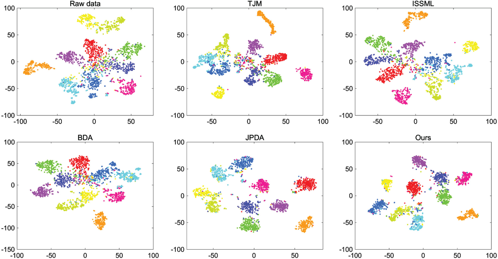
The t-SNE results on the Office+Caltech-256 dataset for the case C→A (DeCAF₆).

As presented in Table 2, overall, our method achieves the highest average classification accuracy of 53.49% on Office+Caltech-256 (800-dim SURF), which is 1.58% higher than the best baseline DIA. Individually, DIA does achieve great performance by leveraging the class discriminative information for some tasks. However, it is worth noting that for tasks C→D and C→W, our method outperforms DIA with 9.62% and 5.46% improvement, respectively. Furthermore, our method achieves the best performance in 6 out of 12 tasks (W→D, D→W, D→C, C→D, C→W and A→W). For tasks D→A and W→C, the gaps between our performance and optimal performance are negligible (0.09% and 0.21%, respectively). Therefore, it can be considered that our method performs excellently in 8 out of 12 tasks, demonstrating its effectiveness.

Table 3 displays the classification accuracy on the Office+Caltech-256 dataset (4096-dim DeCAF₆). Our method outperforms all baseline methods, achieving an average classification accuracy of 90.27%, which exceeds the second-best methods UTML and JPDA by 1.51%. Also, our method performs best in 7 out of 12 tasks (W→D, D→W, C→D, C→A, A→W, A→D and A→C). Notably, for task D→A, our method achieves an accuracy of 91.23%, closely approaching the optimal performance of 91.44%. Compared with baseline methods, our method shows superior performance in mosttasks.

The classification results on the ImageCLEF-DA dataset are reported in Table 4. It can be seen that the performance of our method is superior to all comparison methods and achieves the best performance in 4 out of 6 tasks. Additionally, our method attains the highest average accuracy of 87.20%, surpassing the best baseline UTML by 1.56%.

Furthermore, to present the performance of our approach more intuitively, we visualize the results for cross-domain task C→A (DeCAF₆) of Office+Caltech-256 using the t-SNE [43] tool. As shown in Fig. 2, compared with other approaches, our model exhibits superior intra-class compactness and inter-class separability.

From the above comparative results, we observe that: (1) Compared with all baselines, our method achieves remarkable performance on all datasets and performs best on most tasks. (2) All domain adaptation and metric learning approaches improve the 1NN classification accuracy on all cross-domain tasks, which demonstrates the effectiveness of adopting domain adaptation and metric learning. (3) Comparing Tables 2 and 3, it is clear that classification results are affected by feature types, and all the methods perform better on deep features than on traditional features.

Finally, we discuss the main differences between our method and the other comparison methods: (1) PCA and ISSML are two metric learning approaches which assume the training and testing data follow the same or similar distributions, limiting their performance when facing samples with distribution discrepancies. (2) JDA, BDA, JPDA and DIA are four distribution alignment-based algorithms that reduce the domain shift, but they only perform domain-wise alignment and class-wise alignment. Our method introduces metric learning to address cross-domain tasks from a more meticulous perspective, thus achieving the best performance. (3) Our method outperforms metric learning-based methods CDML, RTML, UTML, MLOT and GMTL, as it selects the optimal subspace dimension automatically and preserves the structure of the data better from the geometric view. (4) Compared with TJM, MTLF and UDA-ALML, our graph-based sample reweighting method is relatively stable.

5.4 Model analysis

In this section, we further study the properties of our proposed method from three aspects: ablation experiments, convergence analysis and parameter sensitivity analysis.

Firstly, to show the impact of each module of our model, ablation experiments are performed on 6 cross-domain tasks. For convenience, we number each term of our objective function as follows: 1) marginal distribution discrepancy; 2) conditional distribution discrepancy; 3) manifold dimension reduction; 4) discrimination improvement; 5) structure regularization; 6) class divisibility; 7) sample reweighting. As reported in Table 5, each term improves the overall classification accuracy to some extent, which explains the rationality of our model. Specifically, when manifold dimension reduction and discrimination improvement terms are added, the classification accuracy increases the most, which further demonstrates the effectiveness of introducing the manifold dimension reduction term and the smooth triplet loss.

Table 5

Ablation experiments for each module on different cross-domain tasks of the Office+Caltech-256 and ImageCLEF-DA datasets. (S) means the feature type is 800-dim SURF, (D) is 4096-dim DeCAF₆. 1) marginal distribution discrepancy; 2) conditional distribution discrepancy; 3) manifold dimension reduction; 4) discrimination improvement; 5) structure regularization; 6) class divisibility; 7) sample reweighting

Module							Cross-domain tasks
1)	2)	3)	4)	5)	6)	7)	D→A (S)	C→W (S)	A→D (D)	W→A (D)	I→P	I→C
√	√						24.11	29.49	73.89	63.47	71.33	88.50
√	√	√					34.03	39.32	85.99	87.79	78.00	94.17
√	√	√	√				35.80	45.08	89.17	88.62	79.00	95.33
√	√	√	√	√			39.98	49.83	90.45	89.35	79.00	95.67
√	√	√	√	√	√		40.29	49.83	90.45	89.67	79.50	95.67
√	√	√	√	√	√	√	40.61	51.86	91.72	89.87	79.67	95.83

Secondly, we validate the convergence of the proposed algorithm by testing the classification error rates of cross-domain tasks: A→W (DeCAF₆), D→A (SURF) and C→I. As shown in Fig. 3, our algorithm converges after 10 iterations and the classification error rates reach a stable level.

Fig. 3

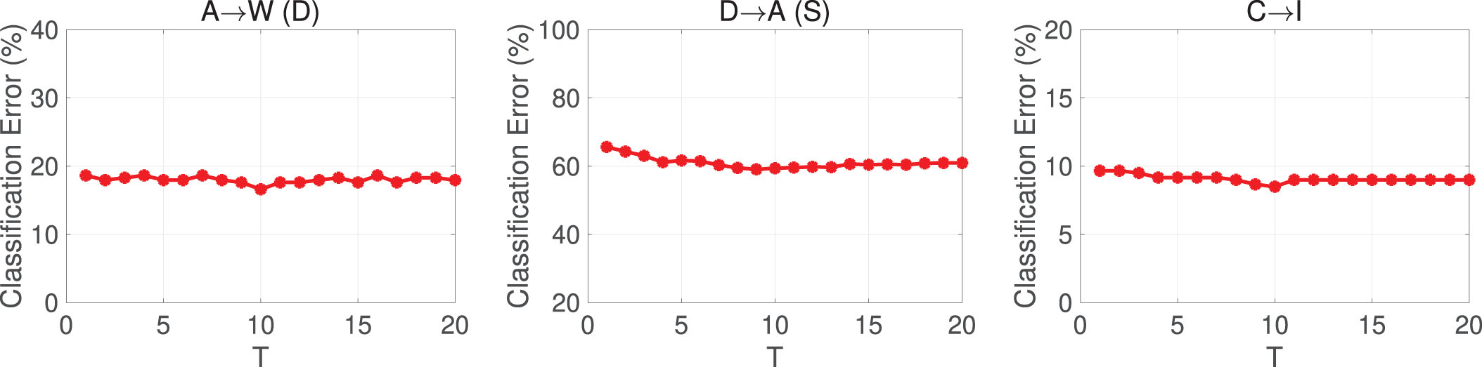
The variation of classification error along with the iteration of the algorithm for the case A→W of Office+Caltech-256 (DeCAF₆), D→A (SURF) and C→I of ImageCLEF-DA.

There are several parameters in our algorithm, i.e., balance parameters α and β in the final objective function, v in calculating the similarity between samples, the bandwidth h, and η in calculating the weight of the source domain sample. To explore the influences of these parameters, we analyze the parameter sensitivity of our method on different types of datasets. Without loss of generality, we choose one task from each of the three datasets as examples, which are A→D of Office+Caltech-256 (DeCAF₆), D→W of Office+Caltech-256 (SURF) and C→I of ImageCLEF-DA, respectively.

Fig. 4 shows the impact of balance parameters α and β ranging in [0.1, …, 0.8] with the step size 0.1. Note that we have α + β < 1 for α and β. In our model, α is the balance parameter of the distribution adaptation and discrimination improvement terms, and β is the balance parameter of the structure preservation term. If the value of α is too small, our model will not take into account the distribution adaptation and discrimination improvement terms. If the value of β is too large, it will cause the model to pay too much attention to the structure preservation term. Therefore, we recommend to select α ∈ [0.3, 0.8] and β ∈ [0.1, 0.6].

Fig. 4

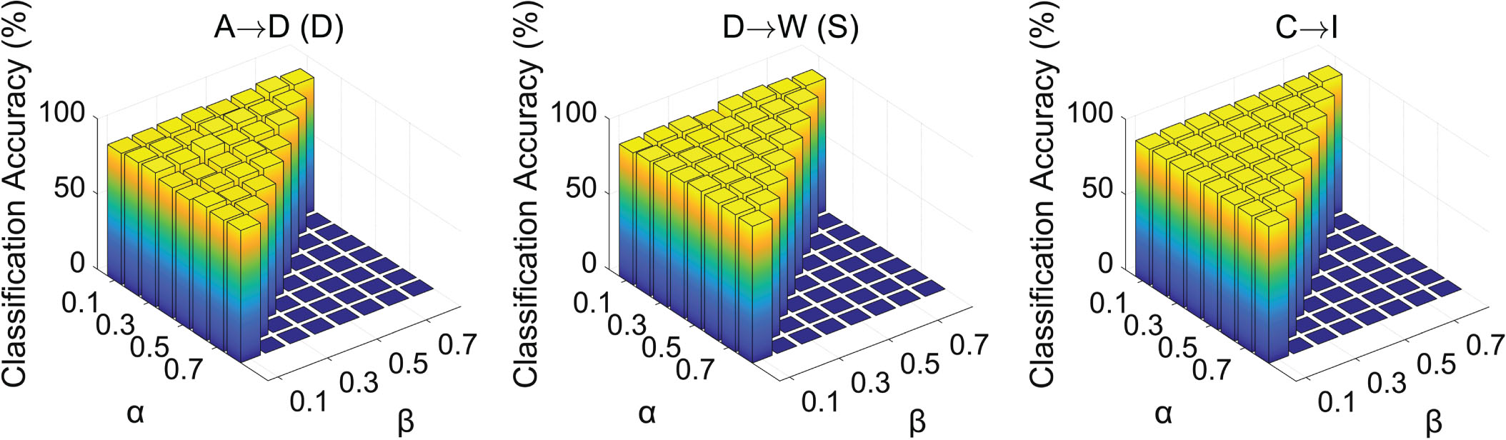
The classification accuracy with varying α and β.

Fig. 5(a) presents the performance of our method under varying values of v. Obviously, v with too-high values will destroy the model performance, and hence v ∈ [1, 5] is the best choice. Fig. 5(b) reveals how the bandwidth h influences the model performance. As shown in Fig. 5(b), the model performance is relatively stable except for task A→D (D). Considering all tasks, we suggest to choose h ∈ [1, 1000] to achieve high performance. In the process of sample reweighting, η controls the number of neighbors when constructing the subgraph. Fig. 5(c) illustrates the effect of the value of η on the model performance. It is clear that the model performs well when η ∈ [0.1, 0.4].

Fig. 5

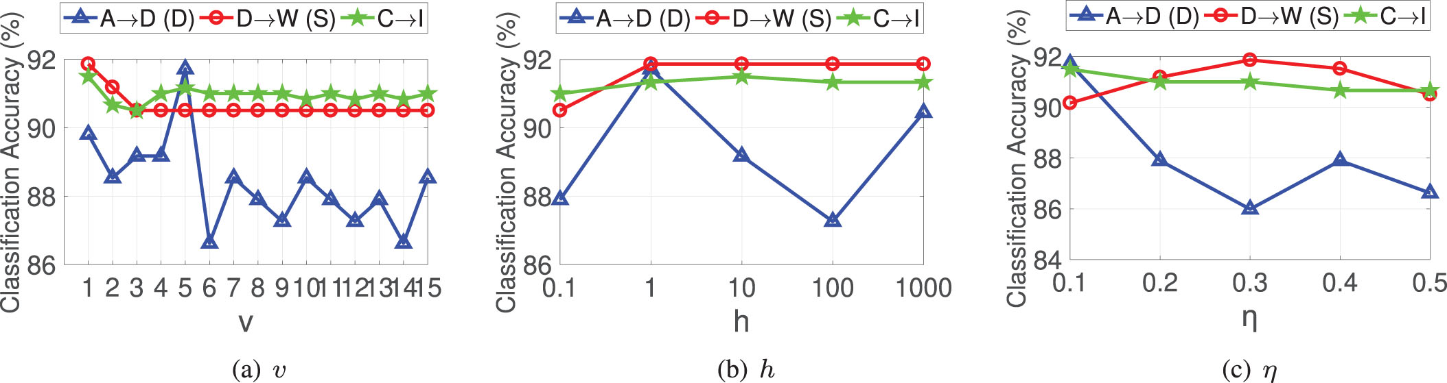
The classification accuracy with varying v, h and η, respectively.

6 Conclusion

In this paper, we propose a coarse-to-fine domain adaptation method based on metric learning. First, to solve the problem that the subspace dimension needs to be set in advance, we automatically select the optimal subspace dimension by using a structure-preserving algorithm on the Grassmannian manifold. Moreover, the separability of data is enhanced by maximizing the MMD distance between different classes. Furthermore, for a finer alignment, we improve the discrimination and preserve the geometry of data by introducing the smooth triplet loss and structure regularization. Finally, a graph-based sample reweighting method is employed to identify the importance of each source domain sample. Extensive experimental results validate the superiority of our approach.

The advanced utilization of geometric structure and sample-wise information in our method brings about excellent performance in alignment. Further, our novel ideas have the potential to transfer into the realm of deep learning. Possessed by the powerful learning ability of deep learning, massive input data issues can be effectively coped with. Therefore, as a future topic, integrating our model with deep learning holds promise and merits further investigation.