Sage Journals: Discover world-class research

Abstract

Predicting the landslide-prone area is critical for various applications, including emergency response, land planning, and disaster mitigation. There needs to be a thorough landslide inventory in current studies and appropriate sampling uncertainty issues. Landslide risk mapping has expanded significantly as machine learning techniques have developed. However, one of the primary issues in Landslide Prediction is data imbalance (DI). This is problematic since it is challenging or expensive to generate an accurate inventory map of landslides based on previous data. This study proposes a novel landslide prediction method using Generative Adversarial Networks (GAN) for generating the synthetic data, Synthetic Minority Oversampling Technique (SMOTE) for overcoming the data imbalance problem, and Bee Collecting Pollen Algorithm (BCPA) for feature extraction. Combining 184 landslides and ten criteria, including topographic wetness index (TWI), aspect, distance from the road, total curvature, sediment transport index (STI), height, slope, stream, lithology, and slope length, a geographical database was produced. The data was generated using GAN, a Deep Convolutional Neural Network (DCNN) technique to populate the dataset. The proposed DCNN-BCPA approach findings were merged with current machine learning methods such as Random Forests (RF), Artificial Neural Networks (ANN), k-Nearest Neighbours (k-NN), Decision Trees (DT), Support Vector Machine (SVM), logistic regression (LR). The model’s accuracy, precision, recall, f-score, and RMSE were measured using the following metrics: 92.675%, 96.298%, 90.536%, 96.637%, and 45.623%. This study suggests that harmonizing landslide data may have a substantial impact on the predictive capabilities of machine learning models.

Keywords

Bee collecting pollen algorithm data balancing generative adversarial network landslide susceptibility synthetic data

1 Introduction

One form of a natural hazard that poses a major risk to both humanity and the environment is landslides [1]. Most landslides are triggered by a single, extremely high rainfall event, an earthquake, human activity, or a trend of persistent rainfall (weeks or days for slow-moving deep-seated landslides, for example). Landslides can be caused by many things, including volcanic activity, rapid snowmelt, and excessive water levels [2]. Hilly areas see more landslides than low-lying ones do. Gravity, stronger at higher inclinations, causes the material to “drag” down the hill. Landslides start to happen when the resistive force reaches a specific point based on the object’s strength, the frictional characteristics of the slide materials and the rock, or a combination of both. Over 70% of catastrophic landslides worldwide result from overly wet circumstances in the Himalayan region [3]. Periodic rains frequently create Himalayan landslides, occasionally resulting in fatalities [4] and inflicting significant financial damages. Froude and Petey’s compilation of a database of fatal landslides revealed 64 fatalities in Bhutan between 2004 and 2017. Yet, it’s believed that there were more casualties overall. As hills are cleared of their vegetation and cut down, the threat is anticipated to rise, highlighting the significance of infrastructure development in light of populace development.

The geographic forecast of landslides is essential in developing landslide risk maps [5]. At this point, landslide inventory levels that offer a geographic map of the risk of landslide measures are used, along with statistical or machine learning representations, to take into account and assess an amount of landslide-conditioning [6].

Statistical and machine learning methods have been heavily utilized in studies on the geographic prediction of landslides [7]. The studies cover a wide variety of topics and focus on several issues, such as Data Imbalance (DI), model evaluation, factor normalization methods, sampling techniques [8], creating training and test samples [9], model assembly [10–11], fine-tuning perfect hyperparameters [12], modeling with limited information, and modeling with limited data. To obtain more accurate prediction of Longitudinal dispersion coefficient (LDC), general structure of group method of data handling (GMDH) is modified by means of extreme learning machine (ELM) conceptions. In fact, with getting inspiration from ELM, a novel GMDH method, called GMDH network based on using extreme learning machine (GMDH-ELM), is proposed in which weighting coefficients of quadratic polynomials applied in conventional GMDH are no longer required to be updated either using back propagation technique or other evolutionary algorithms through training stage [13]. Recent efforts to use machine learning approaches to explore biomarker and clinical marker signatures for optimal management using different clinical cohorts (with almost same number of patients) have shown that the markers [14].

The DI problem in predicting landslides is the main problem with the current study. With landslide spatial projections, DI is a concern. The dataset for landslides comprises two training. The negative class typically outnumbers or underrepresents the positive type. In other words, there is not an equal distribution of both beneficial and adverse justifications. Because they rely on or assume balanced class distributions, most machine learning representations are vulnerable to DI. The classifier becomes more biased in favor of the dominant class; as a result, making it impossible for the algorithms to classify the pixels associated with landslides correctly. Reducing the imbalance consequence in the landslide dataset, then, is crucial. Oversampling a minority lesson and undersampling a majority period are the top strategies for removing imbalance. Many methods, including intelligent under-sampling [15], synthetic sampling with data generation, and random over- and under-sampling, have been employed by numerous scientists to manage DI.

The Generative Adversarial Networks (GAN) used in this study to create the synthetic data, the Synthetic Minority Oversampling Technique (SMOTE) to solve the information imbalance issue, and the Bee Collecting Pollen Algorithm (BCPA) to extract the features all work together to propose a novel landslide prediction method. 184 landslide and 10 criteria, slope, aspect, comprising height, topographic wetness index (TWI), slope length, overall curvature, closeness to a road, lithology, proximity to a stream, and hydrogeologic index, were used to create a geographic database. Data were pooled to fill the dataset, and a Deep Convolutional Neural Network (DCNN), a subtype of GAN, was utilized. After that, the results of the suggested DCNN-BCPA strategy were coupled with commonly used machine learning techniques such as random forests, Artificial Neural Networks (ANN), k-Nearest Neighbors, decision trees, and support vector machines (SVM). Metrics such as the F1-score, Kappa Index, Area Under Receiver Operating Characteristic Curves (AUROC), and Overall Accuracy (OA) were utilized to evaluate the model. Our study demonstrates how balancing landslide information significantly impacts the machine learning algorithms’ ability to predict landslides.

The respite of the paper is organized as surveys: in Unit 2, we analyze studies that have previously addressed problem identification and research limitations. We outline the proposed algorithm and privacy analysis in Unit 3. The investigational findings are accessible and deliberated in Unit 4. Unit 5 provides the conclusions and references for additional study.

2 Literature survey

Tsangaratos et al. [16] The general issue of DI in machine learning with real-world datasets is not an exception when predicting landslides. Because landslides usually have a restricted number of pixels and are documented in network/grid raster spatial data, landslide databases need to be more balanced. Due to the model’s bias towards the dominant class, this problem affects how well machine learning models predict outcomes. By balancing the dataset, it can be avoided.

Song et al. [17] used a DI learning problem to analyze the challenge of predicting the geographic distribution of landslides. They used a method that addresses the algorithmic aspects of the DI problem by employing a cost matrix designed to make the misclassification cost of the negative samples higher than that of the positive ones. Due to this, misclassifying negative samples as positive samples now comes with a higher penalty.

Zhang et al. [18].’s integration of the adaptive synthetic (ADASYN) sampling process with linear discriminant analysis (LDA) for acoustic prediction of landslides improved the results of sample imbalance-influenced modeling. This was carried out to foresee seismic landslides using seismic data. The DI problem has been approached algorithmically in many studies.

Agrawal et al. [19] associated synthetic versus random oversampling. SMOTE and SMOTE-IPF. They projected that synthesized oversampling outperformed random oversampling based on the results of an analysis using a variety of models based on machine learning, including logistic regression (LR), discrete tree (DT), random forest (RF), support vector machines (SVM), and neural networks (NN).

Haixiang et al. [20] Oversampling the minority class by sample duplication or data manipulation artificially boosts the number of landslide records. On the other hand, the standard period technique aims to decrease the examples of the typical period by purposefully (or randomly) choosing a lesser subset from the innovative dataset. To achieve the required class balance, a randomly selected minority class instance is regularly cloned. Synthesized oversampling goes beyond random sampling by creating new artificial minority class examples by interpolating among multiple similar existing minority class examples.

The capacity of machine learning models to predict spatial landslides was examined by Braun et al. [21] concerning data balance. According to their findings, applying data balancing to the training set that is, enhancing the information density of the proper optimistic essentially had no impact on the DT model’s overall performance. However, the model’s performance changed when the test data were applied. This indicates that using a single data point from a landslide to predict where it will occur in space suggests that the model’s capacity to extrapolate the established parameters to novel situations was constrained.

By analyzing the effects of the lack of landslides (negative samples) on the models, Conoscenti et al. [22] performed landslide susceptibility mapping. To determine the absence of landslides, they used randomly positioned circles with a diameter equivalent to the mean length of the landslide source areas. The non-landslide zones were determined by distributing the constituent grid cells similarly randomly (absence selection). The absences selection method used in this paper’s experiments, which used multivariate adaptive regression splines, proved much better than the alternative method when the learning and validation samples were taken from the same region. However, no discernible difference was found when the models were tested outside the training region.

Kalantar et al. [23] investigated how various landslide samples affected SVM, LR, and ANN techniques. Reveals that the randomization significantly impacts the susceptibility models in the training sample selection. The experiment using training samples was documented in a paper, and the findings indicated that the LR perfect is less complex than the SVM and the ANN representations.

Cheng et al. [24] proposes to develop a machine-learning method for predicting landslide areas in the Tsengwen River Watershed (TRW), one of the most landslide-prone regions in Central Taiwan. From 2009 to 2015, diverse spatial datasets were collected to extract 36 predictive variables for landslide modeling using random forests (RF). In comparison to ground reference data, the results of landslide prediction indicated an overall accuracy of 91.4% and a Kappa coefficient of 0.83. Estimates of predictor importance also revealed to officials that the land-use/land-cover (LULC) type, distance to previous landslides, distance to roads, bank erosion, annual groundwater recharge, geological line density, aspect, and slope are the most influential triggers of landslides in the study region.

Thi Ngo et al. [25] we used two novel deep learning algorithms, the recurrent neural network (RNN) and the convolutional neural network (CNN), to map the avalanche susceptibility of Iran at the national scale. To construct a geospatial database, we compiled a dataset containing 4069 historical landslide locations and 11 conditioning factors (altitude, slope degree, profile curvature, distance to river, aspect, plan curvature, distance to road, distance to fault, rainfall, geology, and land-sue) and divided the data into a training dataset and a testing dataset. Using the training dataset, we then developed RNN and CNN algorithms to generate landslide susceptibility maps of Iran. Using the testing dataset, we determined the receiver operating characteristic (ROC) curve and the area under the curve (AUC) for the quantitative evaluation of the landslide susceptibility maps. The RNN algorithm (AUC = 0.88) delivered superior performance in both the training and testing phases when compared to the CNN algorithm (AUC = 0.85).

Bui et al. [26] To predict landslides, we devised the ABSGD ensemble model, which is a combination of a functional algorithm, stochastic gradient descent (SGD), and an AdaBoost (AB) Meta classifier. We ranked 20 landslide conditioning factors using the least-square support vector machine (LSSVM) method. For the modeling, we considered 98 locations of landslides, of which 70% (79) were used for training and 30% (19) were used for validation. Model validation was performed using sensitivity, specificity, accuracy, the root mean square error (RMSE) and the area under the receiver operatic characteristic (AUC) curve. For model validation and comparison, we also utilized soft computing benchmark models, including SGD, logistic regression (LR), logistic model tree (LMT), and functional tree (FT) algorithms.

Nam and F. Wang. [27] a novel deep learning-based algorithm that combine classifiers of both deep learning and machine learning is proposed for landslide susceptibility assessment. A stacked autoencoder (StAE) and a sparse autoencoder (SpAE) both consist of an input layer for raw data, hidden layer for feature extraction, and output layer for classification and prediction. As a study case, Oda City and Gotsu City in Shimane Prefecture, southwestern Japan, were used for susceptibility assessment and prediction of landslides triggered by extreme rainfall. The results show that the prediction ratio of the combined classifiers was 93.2% for StAE combined with RF model and 92.5% for SpAE combined with RF model, which were higher than those of the SVM (87.4%), RF (89.7%), StAE (84.2%), and SpAE (88.2%). The comparative of the existing methods are discussed in Table 1.

2.1 Limitations

“Landslide Data Balancing and Spatial Prediction” is a method that aims to balance unbalanced landslide data and make spatial predictions of landslide susceptibility. However, there are several drawbacks to this strategy, which include the following:

Quality of input data: The accuracy of the landslide vulnerability charts produced by this methodology heavily depends on the input data, including the caliber of the landslide inventory and environmental data. The vulnerability maps produced could only be reliable if the input data is quality.

Inherent uncertainty: Because landslide processes are intricate and dynamic, mapping landslide susceptibility is inherently uncertain. This methodology does not consider this uncertainty, which could lead to either overly optimistic or pessimistic results.

Limited applicability: Due to its reliance on landslide and environmental data availability, this methodology may not be applicable in all regions. The outcomes might not be accurate in areas with scant data availability.

Lack of temporal analysis: This methodology only presents a snapshot of the susceptibility to landslides at a particular time. The area’s vulnerability to landslides may be impacted by material changes in the landscape, which are not considered.

2.2 Problem identification

There are two primary difficulties with the “Landslide Data Balancing and Spatial Prediction” problem:

First, Landslide records frequently suffer from a severe class imbalance, with the number of occurrences of landslides being much lower than the number of non-landslide instances. This disparity might be a significant barrier for machine learning and spatial prediction algorithms. Imbalanced data can result in biased model performance, with the model performing well on the majority class (non-landslides) but badly on the minority class (landslides). As a result of this imbalance, predictive accuracy for landslides is lower, and the rate of false negatives (failure to forecast actual landslides) is higher. It is critical to address this class imbalance in order to construct an effective prediction model.

Second, Landslides are impacted by a variety of geographical elements, including terrain, soil composition, precipitation, and land use. These variables are spatially variable and heterogeneous, which means they can change dramatically over short distances. Accurate landslide prediction necessitates accounting for these regional changes, but it also complicates the modeling approach. Traditional machine learning algorithms may not adequately capture spatial dependencies. To account for the spatial aspect of landslide data, specialized techniques such as spatial autocorrelation modeling, geostatistics, or spatial interpolation methods may be required.

The challenge entails creating efficient methods to balance the landslide dataset and enhance spatial prediction precision, which can significantly impact disaster management and land-use planning.

3 Proposed system

3.1 Data collection

The Nilgiris district, situated in the Western Ghats in Tamil Nadu’s northernmost region, is the subject of this study (Fig. 1). Data for this study was gathered from various sources, including historical landslides, official publications, government repositories, and remotely sensed data. The DCNN-BCPA method’s block diagram is depicted in Fig. 1, Generative Adversarial Networks (GAN) are used in this study to create synthetic data, Synthetic Minority Oversampling Method is used to resolve the information disparity issue, and Bee Collecting Pollen Algorithm (BCPA) is used to extract features.

Fig. 1

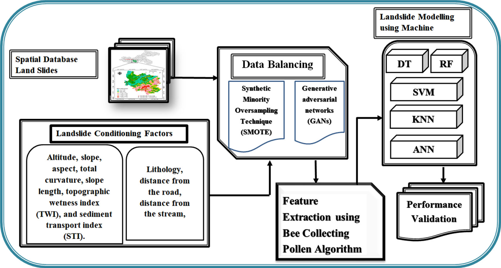
Proposed method of DCNN-BCPA.

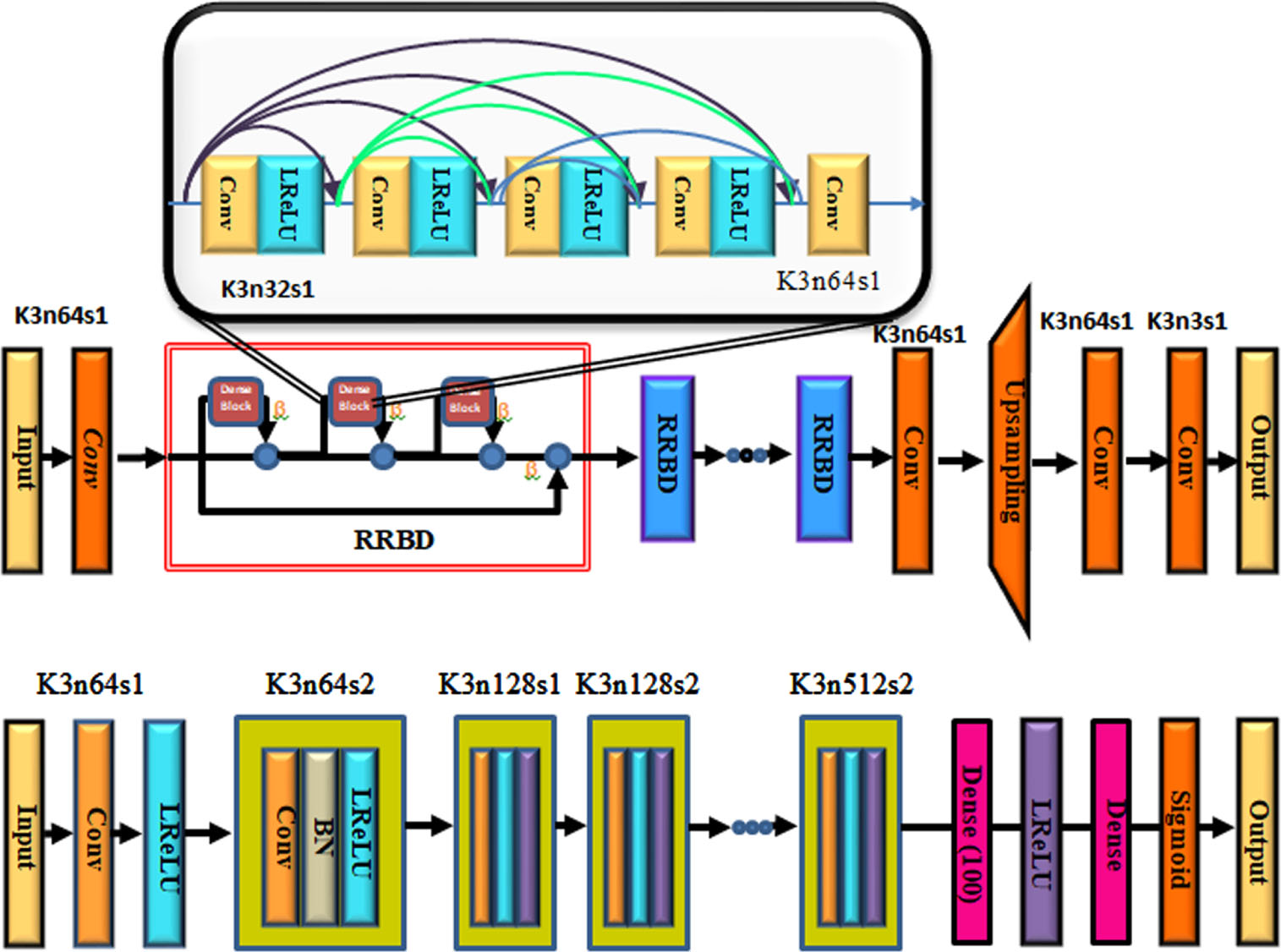
3.2 Landslide conditioning factors

Fig. 2

Generator adversarial networks (GAN) architecture.

Precipitating factors for landslides are total curvature, elevation, aspect, slope, slope length, distance from a road or stream, lithology, topographic wetness index (TWI), and sediment transit index (STI). Vegetation density was considered throughout the landslide prediction process. Using data from Landsat 8 images, the normalized transformation vegetation index was utilized to calculate the vegetation’s amount. The four different forms of vegetation density maps are elevated vegetation, medium-density vegetation, low-density vegetation, and non-vegetation [30]. The following is a list of the equations used to calculate STI and TWI. $STI = {(\frac{A}{22.13})}^{0.6} \times {(\frac{sin β}{0.0896})}^{1.3}$ (1) $TWI = In (\frac{A}{tan β})$ (2) where (in °) is a slope grade and A is identified as a unique region of the reservoir (m2/m); β in radians.

3.3 Data balancing

3.3.1 Synthetic minority oversampling technique (SMOTE)

The first step is to identify the k nearest neighbors of each minority example. SMOTE is regarded as a pre-processing step in landslide susceptibility modeling. After removing DI, it makes it possible to be used on standard machine learning models. The introduced samples may have been interpolated from noisy samples, which prevents SMOTE from effectively handling noise. As a result, data cleaning must be improved after using SMOTE [31].

3.3.2 Utilizing generative adversarial networks, more data creation

The concept of two networks competing underlies generative adversarial networks (GANs). To create synthetic training data that resembles accurate training data, one of the networks is in charge of learning to approximate the distribution that generated the precise training data. In instruction to resolve the adversarial min-max problematic, a Discriminator network D_D and Generator network G_G must be defined. The competition between the two networks can be compared to a min-max game where two players compete to outwit one another. $\begin{matrix} min_{G} max_{D} E_{I^{HG} \sim P_{training} (I^{HG})} [log D_{D} (I^{HG})] \\ + E_{I^{LG} \sim P_{G} (I^{LG})} [log (1 - D_{D} (G_{G} (I^{LG})))] \end{matrix}$ (3)

3.3.2.1. Generator

Step 1. By feeding real data I^LG into Generator, the artificial data G_G (I^LG) is produced. Comparing G_G (I^LG) ‘s discriminant result with 1 yields the loss. This loss reveals whether the Generator’s created image can fool the Discriminator.

Step 2. To extract the features of two datasets, feed the Visual Geometry Group (VGG) feature extraction network the real image I^HG and the artificial data G_G (I^LG). In order to calculate the loss, the characteristics of G_G (I^LG) are contrasted with those of the actual image I^HG. Keep in mind that the Generator training process necessitates a new set of I^HG and I^HG. There are three substantial modules between the generator’s input and output.

A Conv layer with 33 kernels and 64 features, as well as a ReLU layer that provides an activation function. The structure for B-residual blocks presented by Gross and Wilber comprises two sets of Conv layers, each with 33 kernels and 64 characteristics, a Convolution layer, and a ReLU layer acting as the activation function. All blocks, except the last, add the input to the output using the residual connection known as Elementwise-Sum. A further residual reference was made for the previous block’s Elementwise-Sum by connecting the first block’s input to its output. Each Deconv layer consists of two Deconv layers, one Conv layer, two Pixel Shuffler layers, and one ReLU activation layer.

3.3.2.2. Discriminator

The discriminator network is responsible for determining whether an input image is natural or artificial, contributing to the denoised data’s appearance. Since the value of generated samples is close to zero, the Discriminator Network must assign the highest possible probability value to actual image data. To create the real image and the artificial image G_G (I^LG), adjust the results of I^HG and G_G (I^LG) to 1 and 0 respectively.

When the discriminator receives the inputs I^SG or I^HG, it generates judgement results that show whether the input is a genuine dataset or a fake one.

Activation function is a Leaky ReLU combined with a Conv layer.

Seven blocks contained a leaking ReLU layer, a BN layer, and a Conv layer that was repeated. Each block’s kernel size increased between 64 and 512 bytes cyclically, while the strides alternated between 2 and 1.

Another dense activation layer surveys a leaking ReLU layer before the thick, fully connected layer is surveyed. Channel number adjustment is the role of the fully linked layer. The final fully connected layer produces (None, 32, 32, 1), or 1024 discriminations, as its output. The distinctions of an image are then ascertained by averaging the 1024 results.

Loss function:

The typical loss function maximizes mean squared error while minimizing the peak signal-to-noise ratio. The loss function was split into two parts— one for content loss and the other for adversarial loss. ${loss}^{SG} = {loss}_{X}^{SR} + 10^{- 3} {loss}_{Gen}^{SG}$ (4)

${loss}_{X}^{SR}$ stands for adversarial loss, and $10^{- 3} {loss}_{Gen}^{SG}$ stands for content loss.

Content Loss:

The content loss ${loss}_{X}^{SR}$ on MSE is calculated pixel-by-pixel as ${loss}_{MSE}^{SG} = \frac{1}{r^{2} WH} \sum_{x = 1}^{rW} \sum_{y = 1}^{rH} {(I_{x, y}^{HG} - G_{G} (I^{LG})_{x, y})}^{2}$ (5)

The feature representation of the synthetic dataset G_G (I^LG) and the actual dataset I^HG are separated by a Euclidean distance known as the VGG loss. ${loss}_{MSE}^{SG}$ is enhanced by this VGG loss definition. The Euclidean distance for each layer of the feature mapping is calculated using the data from the Generator and the VGG network: ${loss}_{VGG / i, j}^{SG} = \frac{1}{W_{i, j} H_{i, j}} \sum_{x = 1}^{W_{i, j}} \sum_{y = 1}^{H_{i, j}} {(φ_{i, j} (I^{HG})_{x, y} - φ_{i, j} (I^{LG}))_{x, y})}^{2}$ (6)

The individual feature’s sizes within the VGG network are denoted by W_i,j and H_i,j, correspondingly. It is assumed that φ_i,j was passed on to the i-th max-pooling layer before it passed on to the j-th Conv feature-map.

Adversarial Loss:

The output probability of the Generator is used to build the GAN’s loss function. The researchers intend to confuse Discriminator when it assesses images produced by Generator by incorporating GAN adversarial loss. ${loss}_{Gen}^{SG} = \sum_{n = 1}^{N} - log D_{D} (G_{G} (I^{LG}))$ (7)

The probability that G_G (I^LG) was mistreated as I^HG by the discriminator is represented by D_D (G_G (I^LG)).

Table 1

Existing methods of DCNN-BCPA

Author	Method	Objective	Dataset	Landslide target
Y.-S. Cheng et al. [24]	RF	Prediction of landslides using random forests in the Tsengwen River Watershed, Central Taiwan	Tsengwen River Wastershed, Central Taiwan	Susceptibility
P. T. Thi Ngo et al. [25]	RCNN and CNN	Iranian landslide susceptibility mapping at the national level: evaluation of deep learning algorithms	Iran	Susceptibility
D. T. Bui et al. [26]	ABSGD, SGD, LR, LMT,FT	Shallow landslide prediction using a novel hybrid functional machine learning algorithm	Sarkhoon, watershed,Iran	Susceptibility
Nam and Wang in [27]	RF,SVM,DEM,st-AE,sp-AE	Extreme rainfall-induced landslide inventory assessment in Shimane Prefecture utilizing auto encoder and random forest	Shimane Prefecture, Japan’s Oda City and Gostu City	Susceptibility
H. Pei et al. [28]	CNN with Moth flame optimization	A unique hybrid model and convolutional neural network are used to forecast the displacement of landslides while taking time-varying parameters into account.	Lai chau province in Vietnam	Susceptibility
F. Huang et al. [29]	BPNN, Connected Sparse Autoencoder, and SVN are 3 methods (FC-SAE)	Deep learning method using a densely integrated sparse auto decoder neural network for forecasting landslide susceptibility	China’s Guizhou province’s Sinan Country	Susceptibility

3.4 Feature extraction using the bee collecting pollen algorithm

This section describes landslide data balancing and spatial prediction algorithms motivated by honeybee colony behavior. The difficulty lies in modifying the colony’s self-organization behavior to address data balancing and spatial prediction issues related to landslides. Waggle dance and foraging are the two main characteristics of the bee colony when looking for food sources (or nectar exploration). We will review how we relate these aspects of a bee colony to spatial prediction and data balancing for landslides in separate subsections [32, 33].

3.4.1 Waggle dance

Upon returning to the hive from nectar exploration, a forager f_i will effort to achieve waggle dance with probability s and period D = d_iA, where di varies based on profitability rating and A is the waggle dance scaling feature. In addition, with probability, r_i it will attempt to observe and imitate a dance chosen at random. Probability r_i is dynamic and varies based on rating of profitability. A forager will use the dancer’s “path” to find blooming areas if it has decided to follow that dancer. Following indicators left by previous foragers, one can get from the hive to the final destination. The dance will use the forager’s “path,” also called the “preferred path,” to guide its exploration of blooming areas (nectar). To find an optimum medium between landslide data and spatial prediction, it is necessary to link the profitability rating to the objective function. Consider a forager to have a profitability score of Pf I. Originating from: ${Sf}_{i} = \frac{1}{C_{max}^{i}}$ (8)

where $C_{\max}^{i}$ = the make span of the forager f_i’s schedule. The average profitability score for the bee colony, S f_colony, is determined by $S f_{colony} = \frac{1}{n} \sum_{j = 1}^{n} \frac{1}{C_{max}^{j}}$ (9)

Where n is the amount of waggle dances being performed at time t and $C_{\max}^{j}$ is the make span of forager f_j’s waggle dance schedule (we only take dancing bees into account when computing profitability rating). The dance’s length, d_i, is determined by: $d_{i} = \frac{S f_{i}}{S f_{colony}}$ (10)

The profitability ratings in Table 2, are used to modify the probability that a forager or colony will choose a particular path. Foragers are more likely to select randomly to follow a waggle dance if they have a lower profitability rating than the colony.

Table 2

Online resources include the waggle dance probability adjustment table

Profitability score	r _i
s f_i < 0.9 p f_colony	0.60
0.9 S f_colonyS f_i < 0.95 S f_colony	0.20
0.95 S f_colonyS f_i < 1.15 S f_colony	0.02
1.15 S f_colony S f_i	0.00

3.4.2 Forage (Exploration of Nectar)

A populace of l foragers in the colony is provided alongside the algorithm for foraging. These scavengers resolve the spatial prediction and data balancing issues associated with landslides in cycles. The foragers change from node to node along the disjunctive chart’s branches, forming pathways that lead to solutions. A forager needs to travel precisely once from source to sink to each graph node to build a complete solution. Priority restrictions on operations prevent a forager from moving to a node other than those specified in a list of currently permitted nodes while it is at a specific node. The transition probability rule is used by a forager to choose the subsequent node from the list. $S_{ij} (t) = \frac{[ρ_{ij} (t)^{α} . [\frac{1}{d_{ij}}]^{β}}{\sum_{j \in allowed - nosed} [ρ_{ij} (t)^{α} . [\frac{1}{d_{ij}}]^{β}}$ (11)

ρ_ij is the rating of the edge among node_i and node_j, D is the heuristic distance among them, ρ_ij is the likelihood that the edge will branch from them, and so on. ρ_ij is given to the (directed) edge between node_i and node_j. $ρ_{ij} = {\begin{matrix} α \\ \frac{1 - m α}{k - m} \end{matrix}}$ (12) where α is the value given to the preferred pathway, (α<1.0); k is the amount of permitted nodes, m is the amount of desired pathways, and m is either 1 or 0. It should be noted that, according to the expression, ρ_ij will be given the same value for every permitted node during the foragers’ first expedition to find nectar (since m = 0). The α and β parameters change the weighting of edges found on the preferred path in relation to their heuristic distance. This rule states that the likelihood of selecting an edge for the solution increases if it is shorter and located on the preferred path. The processing time of the activities related to node j makes up the heuristic distance. When returning to the hive, a forager that has traversed the entire length of a path will retain the edges it has traversed and the composition of the final waggle dance solution.

3.4.3 The pollution of the environment

Several environmental elements impact the bee’s capacity to collect pollen. The algorithm should get trapped in a local optimum if the best value remains constant. As a result, the algorithm has some control. Adding a random number causes the bee’s position to change independently.

3.4.4 A death

A honeybee only has six weeks left in its life. Every generation, a new populace of bees will be presented to increase exploitation, encourage individual interactions between the old and new populations, and decrease the rate of natural attrition, all of which could increase the search space of the procedure.

3.5 A bulletin

The bulletin records each bee’s optimal choice. Every bee whose position has changed will be compared to the bulletin. The bulletin will be accurate if the change is superior to it. This may result in a worldwide search.

The BCPA is known for efficiently searching the whole solution space. It ensures a thorough search for the best feature subsets by employing many search agents (bees) to collect pollen (solutions) from various locations. With this global search capability, finding high-quality feature combinations is more likely. The BCPA is designed to produce promising results rapidly. It employs a local search strategy, allowing bees to benefit from the surroundings of an existing solution and improve it further. This attribute, as compared to traditional search strategies, speeds up the feature extraction process and enables the speedier acquisition of optimal or nearly ideal feature subsets.

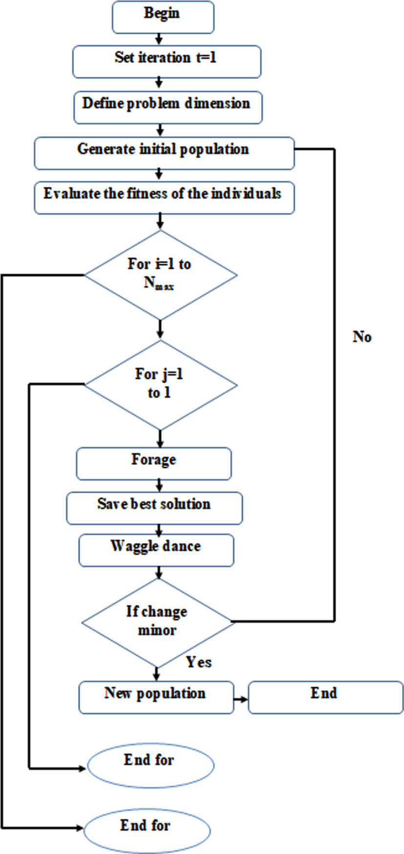
3.6 Algorithmic framework

One cycle (or iteration) of this evolutionary computation approach combines the foraging and waggle dance algorithms. This calculation will run for a predetermined maximum number of iterations, Nmax. The final schedule will be provided at the end of the run utilizing the top solution of the iteration process. The main algorithmic framework of the scheduling method is presented in method 1. Figure 3 depicts the BCPA flowchart.

Algorithm 1. Algorithmic framework for BCPA

Begin

Set iteration t = 1

Define problem dimension

Generate initial population

Evaluate the fitness of the individuals

for i = 1 to N_max

for j = 1 to l

Forage

Save best solution

Waggle dance

if change minor

new population

end if

end for

3.7 Hyperparameter optimization

In addition, categorical attributes typically have a limited set of permitted values, such as the activation function and optimizer options in a neural network. Consequently, the optimization problem is made more difficult because the feasible domain of hyperparameters, denoted by X, frequently possesses a complex structure.

Typically, the goal of a hyperparameter optimization task is to obtain $x * = \arg \begin{matrix} min \\ x \in X \end{matrix} f (x)$ (13)

Fig. 3

Precision evaluation of the DCNN-BCPA method using existing systems.

A hyperparameter, designated x, can take on any value within the search space X. The objective function, f (x), to be minimized may be the error rate or root mean squared error (RMSE). The optimal hyperparameter configuration, x*, produces the highest value for f (x).

The primary HPO technique contains the following phases after selecting an ML algorithm:

Select the performance measures and objective function.

Identify the hyperparameters that require tuning, provide a list of their categories, and choose the optimal optimization procedure.

Train the machine learning model utilizing the default hyperparameter configuration or common values for the baseline.

Start the optimization process with a large search space, determined by manual testing and/or domain expertise, to serve as the feasible hyperparameter domain.

If necessary, investigate additional search spaces or narrow the search space based on the regions where the best functioning hyperparameter values have been evaluated recently.

Finally, provide the hyperparameter configuration that exhibits the best performance.

Traditional optimization strategies built for convex or differentiable optimization issues are frequently inapplicable to HPO problems due to the nonconvex and nondifferentiable character of the objective function in ML models. Furthermore, when the optimization target is not smooth, even certain standard derivative free optimization approaches perform badly.

Because running an ML model on a big dataset can be expensive in HPO techniques, data sampling is sometimes employed to offer estimates of the objective function’s values. As a result, efficient optimization approaches for HPO issues must be able to use these approximations. However, many black box optimization (BBO) approaches do not take function evaluation time into account, making them inappropriate for HPO issues with time and resource constraints. Appropriate optimization methods must be applied to HPO problems in order to discover the optimal hyperparameter configurations for ML models.

4 Result and discussion

In this paper, a unique GAN-based method was presented for advancing training for several existing machine learning models, including support vector machines (SVM), k-nearest neighbors (KNN), decision trees (DT), and random forests (RF) (SVM). Methods for data balancing need to be developed to forecast spatial landslides. The suggested method for data balancing is based on SMOTE and GAN. In the past, GAN models were used to synthesize datasets to boost the effectiveness of machine learning models. These models can analyze a given training dataset’s structure and then generate new data that closely mimics the training data. Uneven data sets can be made more consistent by using additional training samples.

4.1 Analysis of optimization impact on machine learning models

Some hyperparameters significantly impact how well the machine learning models used in this study perform. In this experiment, both the default hyperparameter values and the best-performing values discovered using a randomized search inside a predetermined search space (as described in Table 3) were used. By adjusting the models’ essential hyperparameters, the models were made more precise. These hyperparameters’ common values and each one’s logical minimum and maximum values were used to create the search space. Using cross-validation to get the AUROC accuracy score and determine the best-performing hyperparameter settings, the randomized search approach was used for 20 rounds. Table 3 lists the results of this approach. The studies (conducted in this paper) used these top models compared to the default models.

Table 3
Summary results of optimization of machine learning models

Model (Parameters) Search Space Best Value Validation Score (Std)

Alpha (L2) Activation Function for Hidden Layer Sizes, Max Iteration Learning Rate ANN Solver [LBFGS, SGD, ADAM] (10, 1000, steps:10), –3, 1 range, and (10), power [Adaptive, Constant, Invscaling] [(128,), (64,), (32,), (128, 64), (64, 32), (32, 16), (128, 64, 32), (64, 32, 16), (32, 16, 8)] (–4, 1), (10) power Tanh, ReLU, identity, logistics 650 LBFGS 0.1 Constant (32,) 1.0 Logistic 0.882 (0.007)

RF Estimators Maximum Depth Maximum Features (10, 1000, 10 steps) (2, 15, 10 steps) [Automatic, Sqrt, Log2] 350 8 Log2 0.910 (0.027)

DT Maximum Depth (2, 15, steps:1) 5 0.910 (0.024)

kNN Neighbors (3, 15, steps:1) 6 0.842 (0.008)

Kernel Function SVM C (1, 1000, steps:10) [RBF, Sigmoid, Linear] 81 RBF 0.854 (0.012)

Model (Parameters)	Search Space	Best Value	Validation Score (Std)
Alpha (L2) Activation Function for Hidden Layer Sizes, Max Iteration Learning Rate ANN Solver	[LBFGS, SGD, ADAM] (10, 1000, steps:10), –3, 1 range, and (10), power [Adaptive, Constant, Invscaling] [(128,), (64,), (32,), (128, 64), (64, 32), (32, 16), (128, 64, 32), (64, 32, 16), (32, 16, 8)] (–4, 1), (10) power Tanh, ReLU, identity, logistics	650 LBFGS 0.1 Constant (32,) 1.0 Logistic	0.882 (0.007)
RF Estimators Maximum Depth Maximum Features	(10, 1000, 10 steps) (2, 15, 10 steps) [Automatic, Sqrt, Log2]	350 8 Log2	0.910 (0.027)
DT Maximum Depth	(2, 15, steps:1)	5	0.910 (0.024)
kNN Neighbors	(3, 15, steps:1)	6	0.842 (0.008)
Kernel Function SVM C	(1, 1000, steps:10) [RBF, Sigmoid, Linear]	81 RBF	0.854 (0.012)

4.1.2 Analysis of training data size impact on machine learning models

The quantity of training data influences the efficacy of machine learning models. Several training data sizes were evaluated with the five models employed in this investigation. In addition, various sampling techniques, such as dense, sparse, SMOTE, and GAN, were evaluated with the training data sizes. Generally, the results (as presented in Appendix B) demonstrate that a training size of 0.7 (test data size = 0.3) can achieve good results. Some models, including RF, DT, and k-NN, demonstrated improved accuracy when combined with SMOTE and 0.9 training data size. Other models with smaller training data sizes of 0.5 or 0.3 demonstrated the greatest performance when combined with alternative sampling techniques. However, these outcomes were arbitrary, and no discernible pattern was observed. This study suggests that a training data size of 0.70 should be utilized with the test models.

4.2 Evaluation metrics

Each ground truth pixel’s positions and classes were compared to the corresponding pixels in the classified image to create the confusion matrix.

Accuracy:

The following metrics are used to assess the proposed models’ accuracy:

Accuracy is a common and crucial metric for assessing a prediction representation’s entire presentation. It is the percentage of instances that can be accurately classified with the help of cross-validation data or a different test set. “Eq. (13)” was used in this study to quantify accuracy: $Accuracy = \frac{TP + TN}{TP + FP + TN + FN}$ (14)

False positive, true negative and false negative signals indicate that a model’s pessimistic prediction was incorrect. FP and TN are false positives, and TN for true negative, respectively.

A higher score indicates a model that performs better. The result of averaging the recall (r) and precision (p) scores is F1 (p). Accuracy (p) can be determined by separating the number of true positives by the entire number of pixels (pixels classified as landslides). Sensitivity measures how many accurate positive results can be reliably identified (r). To calculate the value, we divide the entire number of landslide-class pixels by the number of successful matches. Using the formula (14), one can determine their F1-score. $F 1 - Score = 2 \times \frac{p \times r}{p + r}$ (15) $p = \frac{TP}{TP + FP}$ (16) $r = \frac{TP}{TP + FN}$ (17)

There is an issue with the F1-score metric in that it selects positive-biased segments based on a 0.5 threshold. The performance metrics would change if this threshold were altered. One very popular approach to solve his issue is the AUROC curve.

4.3 Machine learning models

Five machine learning models were used to test the proposed DCNN-BCPA-based data balancing method for spatial landslide prediction. The following subsections provide a brief description of these models:

Support Vector Machines (SVM): The SVM, or Support Vector Machine, is a binary classification technique that constructs a separating hyperplane within the original n-dimensional space using the training set points to distinguish between points belonging to two distinct classes. Its goal is to establish the greatest possible margin of separation between these two classes and to locate a classification hyperplane in the centre of this maximum margin. This approach aids in evaluating whether pixels are susceptible (marked as 1) or not susceptible (indicated as –1) to landslides in the context of spatial landslide prediction.

k Nearest Neighbours (kNN): kNN is a non-parametric classification technique that assumes an object’s class roughly reflects the classes of surrounding samples in the vector space. The kNN classifier organizes the neighbours of the sample based on their similarity within the training instances and predicts the new class based on the class labels of the k most similar neighbours. These neighbours’ class labels are weighted based on their similarity, which is assessed using either Euclidean distance or cosine similarity between the vectors.

Decision Trees (DT): The Decision Tree (DT) is a supervised classification system that was created using recursive data partitioning. Each cycle divides the data depending on the values of a given property until the data subsets contain instances from the same class. All input attributes are evaluated at each split in the tree to determine their impact on the attribute being forecasted. Using a DT requires no prior knowledge of data distribution and allows for simple analysis. It is also straightforward to develop and explain, making it accessible to decision-makers in charge.

Random Forests (RF): A forest is made up of many decision trees. Each tree is built with a bootstrap sample from the training set and a random subset of characteristics and samples chosen at each node. This method reduces the correlation between trees by utilizing each tree’s strengths and minimizing reciprocal correlations, making the model less prone to overfitting. Furthermore, as compared to other black-box models such as Neural Networks (NN), the Random Forest (RF) method predicts the relative relevance of the input variables, increasing its explanatory power. Mixed variables, which include both categorical and numerical data, are common in landslide research. As a result, the RF method is well suited to assessing such variables.

Artificial Neural Networks (ANN): ANN, or Artificial Neural Network, is a learning algorithm made up of neurons organized in layers that can be used for classification and regression tasks. Throughout the training process, the algorithm is fed examples on a consistent basis, and the weights are changed to meet the desired objective value. Notably, in landslide investigations, it is not necessary to use a simple method to assess its intended aims.

Table 4 lists the hyperparameters used during the research. Hyperparameters are often used to optimize the fitting process, which can improve the machine learning model prediction accuracy. The goal of picking hyperparameters is to optimize the evaluation values. Different optimizers were utilized to tune the hyperparameters, with some delivering more accurate results than others. For the assessments in the presented study, the grid search technique was applied. The hyperparameters with the highest accuracy were picked for the final training and testing of the individual machine learning models.

Table 4
Hyperparameters for optimal values of the machine learning-based models

Classifier Hyperparameters Explanation

SVM Kernels Gama, Linear

C value Regularization intensity value

DT Max depth Maximum depth of the tree

Random state Controls the randomness of the estimator

RF Generalization error always converges even with increasing number of trees. Larger input datasets will lengthen classification times.

KNN Considered high computational complexity It scales badly, if there are a million labeled examples in the dataset.

heterogeneous distributed points. It would take a long time to find K nearest neighbors when there are a million labeled examples in the dataset.

ANN With a higher number of units of the hidden layer, the network capacity becomes greater to represent the training data patterns. More data would lengthen NN training times to unacceptable levels so that it would be highly impractical to work with them.

Time-consuming parameter tuning procedure.

Classifier	Hyperparameters	Explanation
SVM	Kernels	Gama, Linear
	C value	Regularization intensity value
DT	Max depth	Maximum depth of the tree
	Random state	Controls the randomness of the estimator
RF	Generalization error always converges even with increasing number of trees.	Larger input datasets will lengthen classification times.
KNN	Considered high computational complexity	It scales badly, if there are a million labeled examples in the dataset.
	heterogeneous distributed points.	It would take a long time to find K nearest neighbors when there are a million labeled examples in the dataset.
ANN	With a higher number of units of the hidden layer, the network capacity becomes greater to represent the training data patterns.	More data would lengthen NN training times to unacceptable levels so that it would be highly impractical to work with them.
		Time-consuming parameter tuning procedure.

4.1.1 Precision analysis

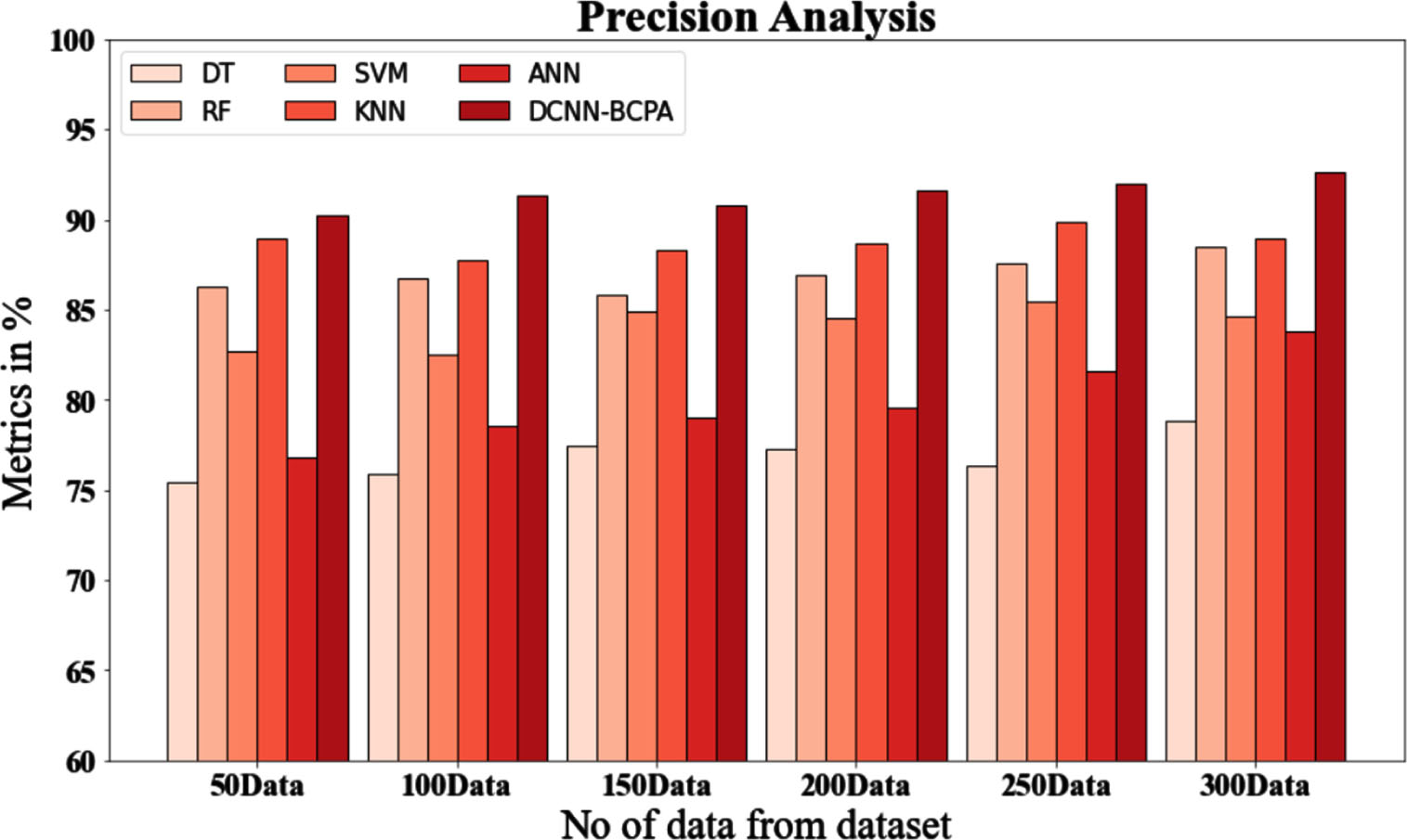
In Fig. 4, and Table 5, comparative precision analyses of the DCNN-BCPA approach and other methods are displayed. The graphic illustrates how performance and precision have increased due to the machine learning method. For example, the DCNN-BCPA model has a precision value of 90.256% with data size 50, whereas the DT, RF, SVM, KNN, and ANN models have accuracy values of 75.436%, 86.294%, 82.738%, 88.937%, and 76.846%. The DCNN-BCPA model, however, has demonstrated its best performance with various data sizes. The precision value of the DCNN-BCPA is 92.675% under 300 data points, compared to 78.826%, 88.536%, 84.632%, 88.964%, and 83.836% for the DT, RF, SVM, KNN, and ANN representations, correspondingly.

Fig. 4

Precision evaluation of the DCNN-BCPA method using existing systems.

Table 5

Precision evaluation of the DCNN-BCPA method using existing systems

No of data	DT	RF	SVM	KNN	ANN	DCNN-BCPA
from dataset
50	75.436	86.294	82.738	88.937	76.846	90.256
100	75.936	86.746	82.536	87.735	78.543	91.345
150	77.502	85.837	84.927	88.325	79.023	90.754
200	77.278	86.937	84.536	88.637	79.574	91.654
250	76.327	87.536	85.501	89.864	81.627	91.954
300	78.826	88.536	84.632	88.964	83.836	92.675

4.1.2 Recall analysis

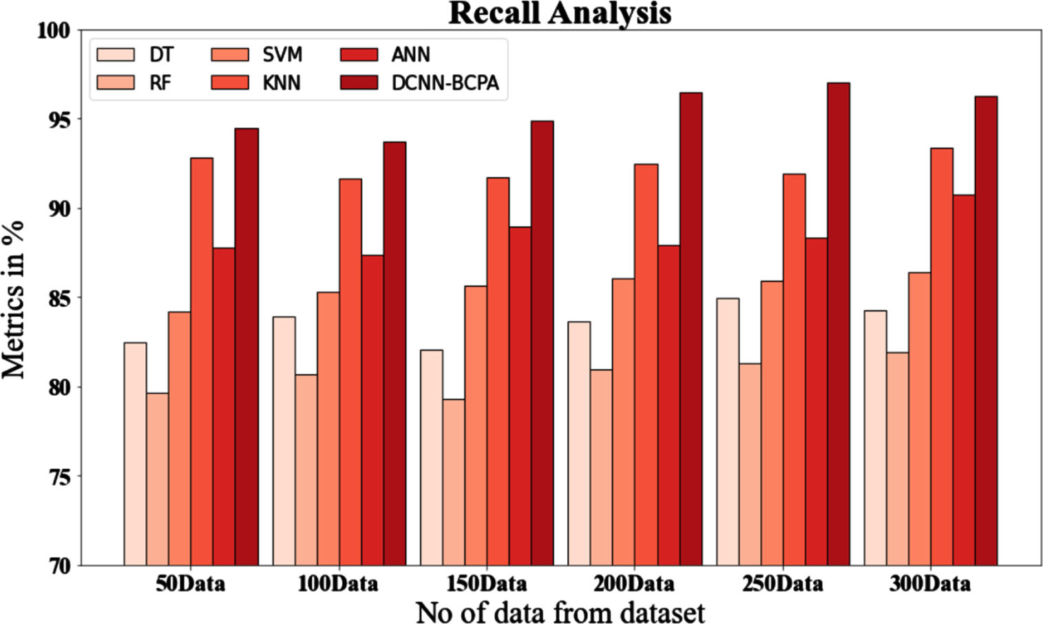
Comparative recall testing of the DCNN-BCPA approach against other available techniques is shown in Fig. 5 and Table 6, The graph shows how the machine learning method enhanced performance and recall. For example, with data size 50, DCNN-BCPA has a recall value of 94.447%, whereas the DT, RF, SVM, KNN, and ANN models have recall values of 82.485%, 79.657%, 84.184%, 92.847%, and 87.758%, respectively. Nonetheless, the DCNN-BCPA model performed well with diverse data sizes. Likewise, the recall value of DCNN-BCPA under 300 data points is 96.298%, whereas the DT, RF, SVM, KNN, and ANN models have recall values of 84.294%, 81.937%, 86.384%, 93.344%, and 90.727%, respectively.

Fig. 5

Recall analysis for the DCNN-BCPA approach with existing systems.

Table 6

Analyze of Recall for the DCNN-BCPA Technique Using Existing Systems

No of data	DT	RF	SVM	KNN	ANN	DCNN-BCPA
from dataset
50	82.485	79.657	84.184	92.847	87.758	94.447
100	83.947	80.647	85.294	91.655	87.342	93.684
150	82.057	79.325	85.648	91.738	88.937	94.924
200	83.647	80.928	86.093	92.475	87.934	96.449
250	84.938	81.294	85.948	91.948	88.346	97.027
300	84.294	81.937	86.384	93.344	90.727	96.298

4.1.3 F-score analysis

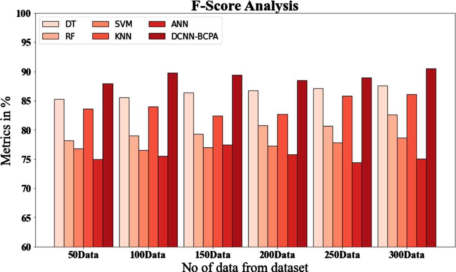
Figure 6 and Table 7, display an f-score comparison of the DCNN-BCPA technique with various known approaches. The graph shows how the machine learning approach has enhanced performance, as indicated by the f-score. With data size 50, for instance, the DCNN-BCPA model’s f-score value is 87.937%, whereas those of the DT, RF, SVM, KNN and ANN models are 85.291%, 78.234%, 76.826%, 83.627%, and 74.937%, respectively. However, the DCNN-BCPA model has performed well across various data sizes. Under 300 data sets, the DCNN-BCPA has an f-score value of 90.536%, whereas the DT, RF, SVM, KNN, and ANN models have 87.536% values, 82.634%, 78.657%, 86.088%, and 75.024%, respectively.

Fig. 6

F-score analysis for DCNN-BCPA method with existing systems.

Table 7

F-score analysis with existing systems for the DCNN-BCPA technique

No of data	DT	RF	SVM	KNN	ANN	DCNN-BCPA
from dataset
50	85.291	78.234	76.826	83.627	74.937	87.937
100	85.538	79.024	76.546	83.947	75.536	89.763
150	86.382	79.274	76.953	82.385	77.435	89.435
200	86.782	80.726	77.245	82.674	75.829	88.536
250	87.132	80.674	77.837	85.826	74.425	88.927
300	87.536	82.634	78.657	86.088	75.024	90.536

4.1.4 Accuracy analysis

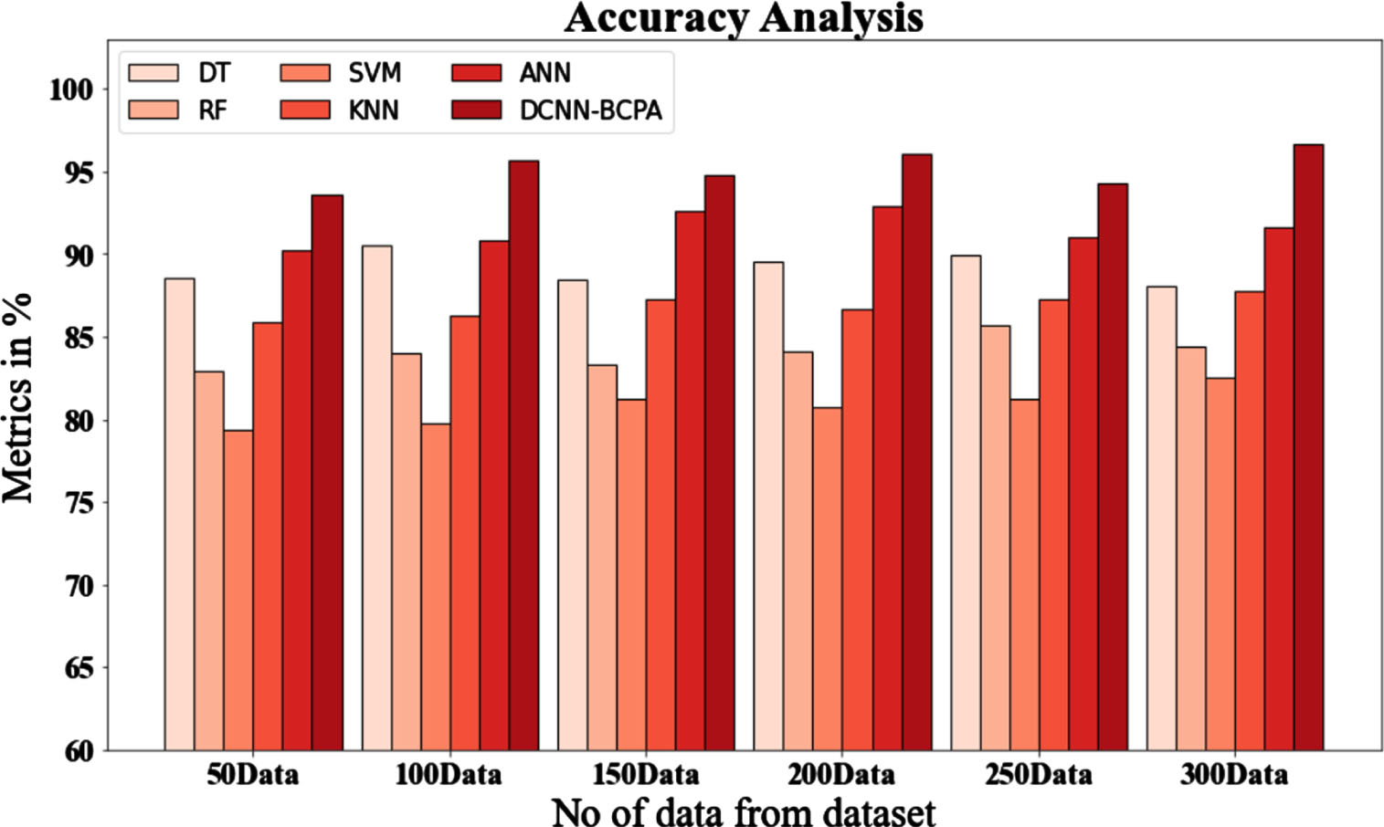
In Fig. 7 and Table 8, comparative accuracy studies of the DCNN-BCPA approach and other methods are displayed. The graph shows that the performance and accuracy of the machine learning technique have increased. For instance, the DCNN-BCPA model has an accuracy of 93.647% with data size 50, compared to 88.536%, 82.875%, 79.345%, 85.932%, and 90.231% for the DT, RF, SVM, KNN, and ANN models. However, the DCNN-BCPA model has been shown to perform the best across various data sizes. Under 300 data sets, the DCNN-BCPA has an accuracy value of 96.637% compared to the DT, RF, SVM, KNN, and ANN models’ accuracy values of 88.026%, 84.356%, 82.543%, 87.734%, and 91.637%, respectively.

Fig. 7

Accuracy analysis of the DCNN-BCPA approach with existing systems.

Table 8

Accuracy analysis of the DCNN-BCPA approach with existing systems

No of data	DT	RF	SVM	KNN	ANN	DCNN-BCPA
from dataset
50	88.536	82.875	79.345	85.932	90.231	93.647
100	90.536	83.965	79.732	86.244	90.839	95.637
150	88.425	83.276	81.288	87.284	92.637	94.829
200	89.536	84.098	80.743	86.683	92.937	96.028
250	89.936	85.674	81.276	87.245	91.045	94.284
300	88.026	84.356	82.543	87.734	91.637	96.637

4.1.5 Training loss and testing loss analysis

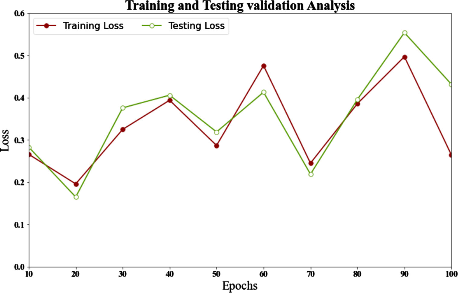
Figure 8 and Table 9, describe the loss analysis of the DCNN-BCPA method with testing and training datasets. According to the figure, the loss for training and testing validation for 10 epochs is 0.266 and 0.283, respectively. Similarly, the loss for training and testing validation for 100 epochs is 0.26 and 0.43, respectively. The resulting data demonstrates that the proposed method has the lowest loss across various periods.

Fig. 8

Training loss and testing loss analysis of DCNN-BCPA method.

Table 9

Analysis of training and testing losses for the DCNN-BCPA method

Epochs	Training loss	Testing loss
10	0.266	0.283
20	0.196	0.165
30	0.325	0.376
40	0.394	0.406
50	0.287	0.319
60	0.476	0.413
70	0.245	0.219
80	0.386	0.396
90	0.497	0.554
100	0.265	0.432

4.1.6 RMSE analysis

The DCNN-BCPA approach is compared to other existing methods using RMSE, as shown in Fig. 9 and Table 10, The graph demonstrates that the technique for machine learning improved performance while reducing RMSE. As an illustration, the DCNN-BCPA model’s RMSE value with 50 data points is 41.836%. However, the DT, RF, SVM, KNN, and ANN models have slightly lower RMSE values of 56.637%, 58.938%, 52.937%, 45.936%, and 48.154%, respectively. On the other hand, the DCNN-BCPA model has demonstrated maximum performance with low RMSE values for a range of data sizes. The RMSE value for the DCNN-BCPA under 300 data points is 45.623%, while the corresponding figures for the DT, RF, SVM, KNN and ANN models are 58.524%, 61.774%, 55.834%, 47.737%, and 52.463%.

Fig. 9

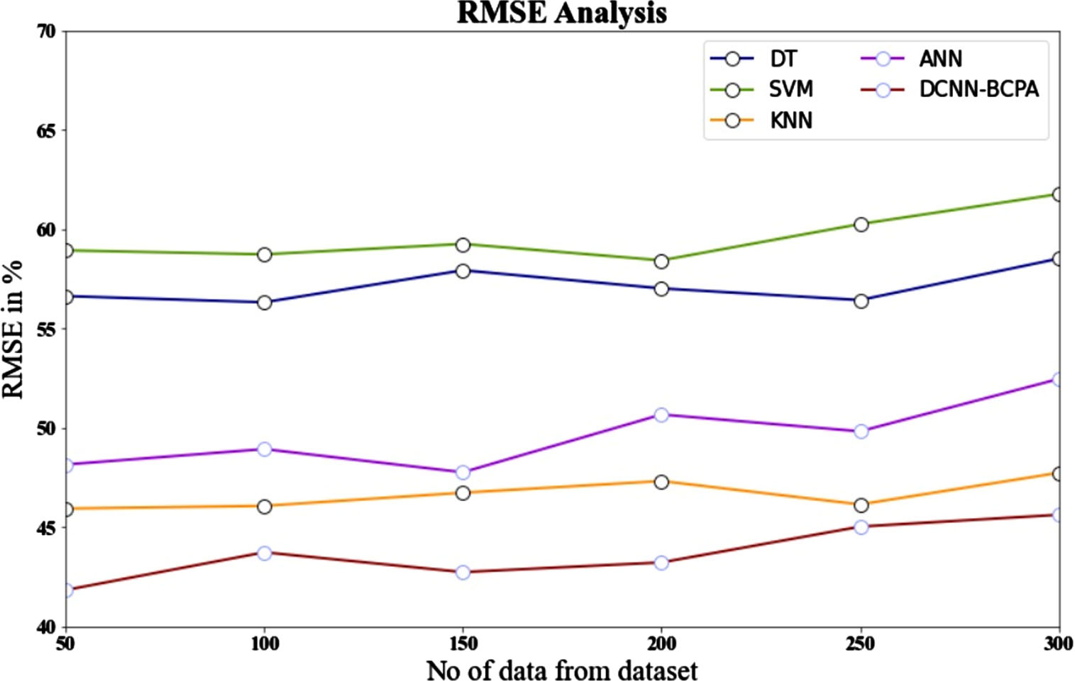
RMSE analysis for DCNN-BCPA method with existing systems.

Table 10

Analyze of the RMSE for the DCNN-BCPA approach with existing systems

No of data	DT	RF	SVM	KNN	ANN	DCNN-BCPA
from dataset
50	56.637	58.938	52.937	45.936	48.154	41.836
100	56.324	58.737	53.746	46.073	48.933	43.735
150	57.937	59.263	52.093	46.736	47.763	42.736
200	57.024	58.435	54.193	47.325	50.673	43.224
250	56.436	60.263	54.837	46.145	49.827	45.028
300	58.524	61.774	55.834	47.737	52.463	45.623

4.2.7 Computational cost analysis

As shown in Fig. 10 and Table 11, the DCNN-BCPA strategy outperforms other existing methods regarding computing cost. For example, the computational cost value of the DCNN-BCPA model with 50 data points is 21.098%. ON THE OTHER HAND, the DT, RF, SVM, KNN, and ANN models have slightly lower computational cost values of 44.566%, 38.244%, 34.988%, 30.233%, and 26.675%, respectively. In contrast, the DCNN-BCPA model has demonstrated maximum performance with low computational cost values across various data sizes. The computational cost value for the DCNN-BCPA under 300 data points is 25.987%, whereas the DT, RF, SVM, KNN, and ANN models are 48.343%, 43.98%, 37.277%, 33.455%, and 28.955%, respectively.

Fig. 10

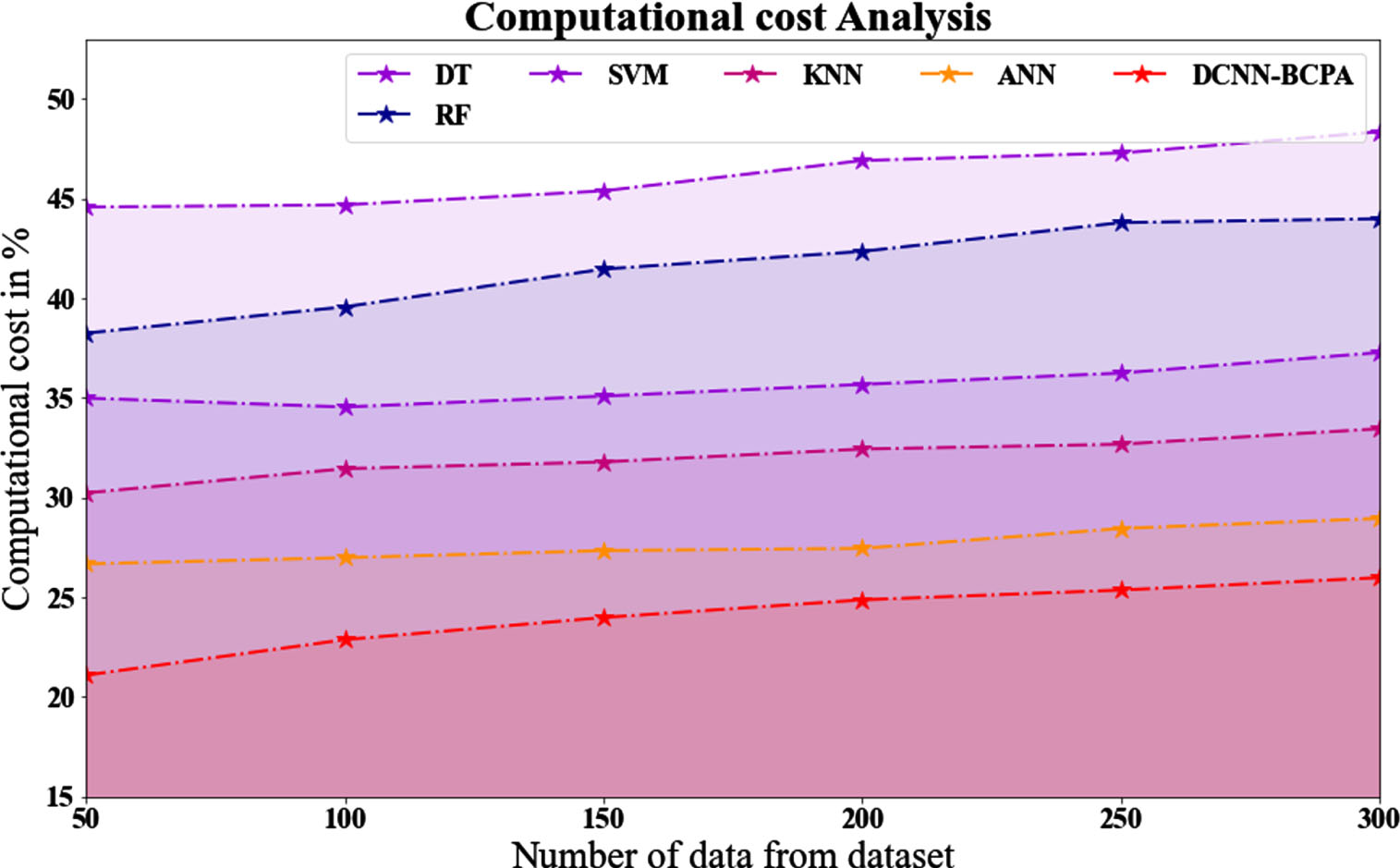
Computational cost Analysis for DCNN-BCPA method with existing systems.

Table 11

Analyze of the computational cost for the DCNN-BCPA approach with existing systems

No of data	DT	RF	SVM	KNN	ANN	DCNN-BCPA
from dataset
50	44.566	38.244	34.988	30.233	26.675	21.098
100	44.677	39.566	34.543	31.453	26.988	22.877
150	45.377	41.456	35.087	31.786	27.344	23.988
200	46.899	42.344	35.675	32.433	27.455	24.876
250	47.277	43.786	36.245	32.677	28.455	25.367
300	48.343	43.98	37.277	33.455	28.955	25.987

4.2.8 ROC-AUC analysis

The AUROC map for the top-performing models balanced with DCNN-BCPA is shown in Fig. 11. These graphs aid in better understanding of the link between the true positive rate and the false positive rate. In this context, a score of 1.0 implies the best AUROC, while a score of 0.5 denotes the worst AUROC. A comparison of the accuracy assessments between the DCNN-BCPA and the benchmark methods demonstrates that the DCNN-BCPA model outperforms other classifiers in predicting landslide susceptibility. The AUROC values calculated for the DCNN-BCPA and benchmark techniques show that the DCNN-BCPA technique has significantly higher accuracy than the benchmarks. This conclusion implies that the features recovered using this method can characterize landslide susceptibility more precisely than the benchmark methods, as measured by the AUROC indices. Notably, the DCNN-BCPA model (with an AUROC of 100%) outperforms individual classifiers such as SVM (with an AUROC of 88%), KNN (with an AUROC of 78%), DT (with an AUROC of 92%), RF (with an AUROC of 95%), and ANN (with an AUROC of 94%), as measured by the recorded indices.

Fig. 11

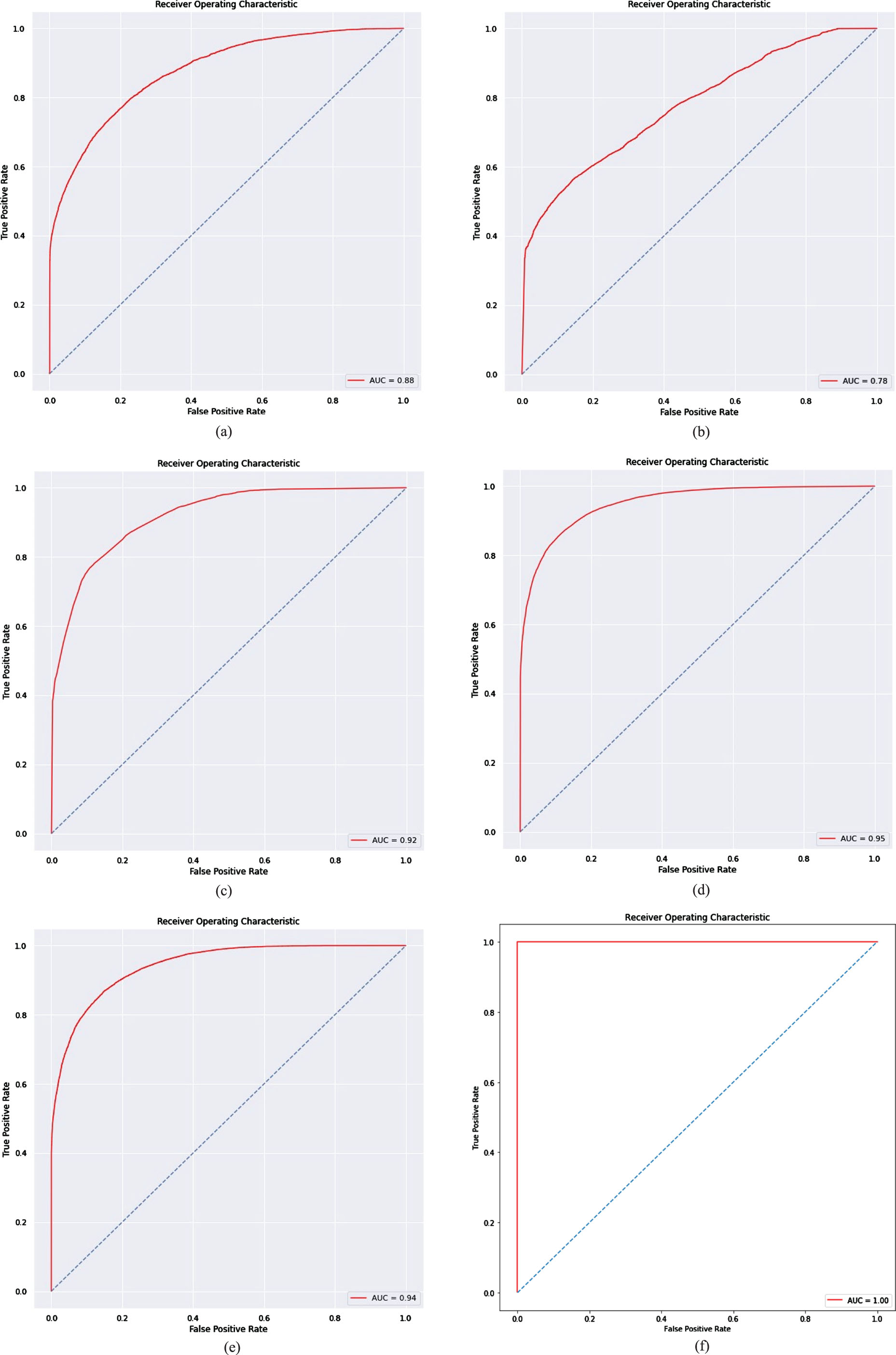
Evaluation of the landslide susceptibility maps based on the AUROC test using: (a) SVM, (b) KNN, (c) DT, (d) RF, (e) ANN and (f) Proposed DCNN-BCPA method.

5 Conclusion

In this article, we provide a novel technique for landslide prediction using Generative Adversarial Networks (GAN) to produce synthetic information, Synthetic Minority Oversampling Technique (SMOTE) to address the problem of information imbalance, and Bee Collecting Pollen Algorithm (BCPA) to extract features. An area-wide database of 184 landslides was constructed using 10 criteria: topographic wetness index (TWI), aspect, distance from the road, total curvature, sediment transport index, height, slope, stream, lithology, and slope length. The dataset was then filled using a GAN called the Deep Convolutional Neural Network after the data were pooled (DCNN). Then, the outputs of the suggested DCNN-BCPA strategy were integrated with or added to those of other machine learning methods currently in use, such as decision trees (DT), random forests (RF), artificial neural networks (ANN), k-nearest neighbors (KNN), and support vector machines (SVM). The model’s accuracy, precision, recall, f-score, and RMSE were measured using the following metrics: 92.675%, 96.298%, 90.536%, 96.637%, and 45.623%. Our research shows that balancing landslide data significantly affects how precisely machine learning algorithms can predict outcomes. Future studies should evaluate the efficacy of Metaheuristic using additional ML methods like RFs and CNNs. The PI-normalized average width (PINAW) and PI-coverage probability (PICP), which are used to judge the suitability of PIs, could also be utilized as inputs for the detection of significant differences in situations with absolute uncertainty. We will be able to comprehend the physical dynamics underlying geohazard modeling better if we combine data-driven models with physical models to create ML models that are explicable and interpretable.

Declarations

Contributions

Aruna Jasmine and J Heltin Genitha contributed to the design and implementation of the research, to the analysis of the results and to the writing of the manuscript.

Data availability

The data used to support the findings of this study are available from the corresponding author upon request.

Conflicts of interest

The authors declare no conflicts of interest.

Funding

The authors received no specific funding for this research.

Ethics approval

Not applicable.

Consent to participate

Not applicable.

References

Turner

A.K.

, Social and environmental impacts of landslides, Innov Infrastruct Solut 3 (2018), 1–25. doi: 10.1007/s41062-018-0175-y.

Mezaal

M.R.

, Pradhan

, Sameen

M.I.

, Shafri

H.Z.M.

and Yusoff

Z.M.

, Optimized neural architecture for automatic landslide detection from high-resolution airborne laser scanning data, Appl Sci 7 (2017), 730. doi: 10.3390/app7070730.

Froude

M.J.

and Petley

D.N.

, Global fatal landslide occurrence from to , Nat Hazards Earth Syst Sci 18 (2018), 2161–2181. doi: 10.5194/nhess-18-2161-2018.

Dikshit

, Sarkar

, Pradhan

, Jena

, Drukpa

and Alamri

A.M.

, Temporal Probability Assessment and Its Use in Landslide Susceptibility Mapping for Eastern Bhutan, Water 12 (2020), 267. doi: 10.3390/w12010267.

Lee

J.H.

, Sameen

M.I.

, Pradhan

and Park

H.J.

, Modeling landslide susceptibility in data-scarce environments using optimized data mining and statistical methods, Geomorphology 303 (2018), 284–298. doi: 10.1016/j.geomorph.2017.12.007.

Yang

, Yang

, Xu

and Song

, Local-scale landslide susceptibility mapping using the B-GeoSVC model, Landslides 16 (2019), 1301–1312. doi: 10.1007/s10346-019-01174-y.

Zhao

and Chen

, Optimization of computational intelligence models for landslide susceptibility evaluation, Remote Sens 12 (2020), 2180. doi: 10.3390/rs12142180.

Lai

J.S.

, Chiang

S.H.

and Tsai

, Exploring influence of sampling strategies on event-based landslide susceptibility modeling, ISPRS Int J Geo-Inf 8 (2019), 397. doi: 10.3390/ijgi8090397.

Pourghasemi

H.R.

, Kornejady

, Kerle

and Shabani

, Investigating the effects of different landslide positioning techniques, landslide partitioning approaches and presence-absence balances on landslide susceptibility mapping, Catena 187 (2020), 104364. doi: 10.1016/j.catena.2019.104364.

10.

Chowdhuri

, Pal

S.C.

, Arabameri

, Ngo

P.T.T.

, Chakrabortty

, Malik

, Das

and Roy

, Ensemble approach to develop landslide susceptibility map in landslide dominated Sikkim Himalayan region, India, Environ Earth Sci 79 (2020), 1–28. doi: 10.1007/s12665-020-09227-5.

11.

Mohan

, Subramani

, Abbas Mardani , Sudhanshu Maurya , Arulkumar

and Thangaraj

, Eagle strategy arithmetic optimisation algorithm with optimal deep convolutional forest based fintech application for hyper-automation, Enterprise Information Systems 17(10) (2023), 2188123. https://doi.org/10.1080/17517575.2023.2188123

12.

Al-Najjar

H.A.

and Pradhan

, Spatial landslide susceptibility assessment using machine learning techniques assisted by additional data created with generative adversarial networks, Geosci Front 12 (2021), 625–637. doi: 10.1016/j.gsf.2020.

13.

Saberi-Movahed

, Najafzadeh

and Mehrpooya

, Receiving more accurate predictions for longitudinal dispersion coefficients in water pipelines: training group method of data handling using extreme learning machine conceptions, Water Resour Manage 34 (2020), 529–561.

14.

Saberi-Movahed

, Mohammadifard

, Mehrpooya

, Rezaei-Ravari

, Berahmand

et al., Decoding clinical biomarker space of COVID-19: exploring matrix factorization-based feature selection methods, medRxiv [Preprint]. 2021 Jul 9:2021.07.07.21259699. Comput Biol Med 146 (2022), 105426.

15.

Cardarilli

, Lombardi

and Corazza

, Landslide risk management through spatial analysis and stochastic prediction for territorial resilience evaluation, Int J Saf Secur Eng 9 (2019), 109–120.

16.

Gupta

S.K.

, Jhunjhunwalla

, Bhardwaj

, Shukla

D.P.

Data imbalance in landslide susceptibility zonation: Under-sampling for class-imbalance learning, Int Arch Photogramm Remote Sens Spat Inf Sci 2020. XLII-3/W11, 51–57.

17.

Song

, Niu

, Xu

, Ye

, Peng

, Guo

, Li

and Chen

, Landslide susceptibility mapping based on weighted gradient boosting decision tree in wanzhou section of the three gorges reservoir area (China), ISPRS Int J Geo-Inf 8(4) (2019).

18.

Zhang

and Yu

, Seismic landslide susceptibility assessment based onADASYN-LDAmodel, In Proceedings of the IOP Conference Series: Earth and Environmental Science, 5th International Conference on Minerals Source, Geotechnology and Civil Engineering, Guiyang, China, 17–19 April 2020; IOP Publishing: Bristol, UK, 525 (2020), 12087.

19.

Agrawal

, Baweja

, Dwivedi

, Saha

, Prasad

, Agrawal

, Kapoor

, Chaturvedi

, Mali

and Kala

V.U.

, A Comparison of Class Imbalance Techniques for Real-World Landslide Predictions, In Proceedings of the 2017 International Conference on Machine Learning and Data Science (MLDS), IEEE., Noida, India, 14–15 1–8, December. 2017.

20.

Steger

, Brenning

, Bell

and Glade

, The influence of systematically incomplete shallow landslide inventories on statistical susceptibility models and suggestions for improvements, Landslides 14 (2016), 1767–1781. https://doi.org/10.1007/s10346-017-0820-0

21.

Haixiang

, Yijing

, Shang

, Mingyun

, Yuanyue

and Bing

, Learning from class-imbalanced data: Review of methods and applications, Expert Syst Appl 73 (2017), 220–239.

22.

Braun

, Garcia-Urquia

E.L.

, Lopez

R.M.

and Yamagishi

, Landslide Susceptibility Mapping in Tegucigalpa, Honduras, Using Data Mining Methods, In Proceedings of the IAEG/AEG Annual Meeting Proceedings, San Francisco, CA, USA, 2018, vol. 1, Springer, Cham, Switzerland, pp. 207–215, 2019.

23.

Kalantar

, Pradhan

, Amir Naghibi

, Motevalli

and Mansor

, Assessment of the effects of training data selection on the landslide susceptibility mapping: a comon between support vector machine (SVM), logistic regression (LR) and artificial neural networks (ANN), Geomatics Nat Hazards Risk 9 (2018), 49–69. https://doi.org/10.1080/19475705.2017.1407368

24.

Cheng

Y.S.

, Yu

T.T.

and Son

N.T.

, Random forests for landslide prediction in Tsengwen River Watershed, Central Taiwan, Remote Sens 13(2) (2021), 199. doi: 10.3390/rs13020199.

25.

Thi Ngo

P.T.

, Panahi

, Khosravi

, Ghorbanzadeh

, Kariminejad

, Cerda

and Lee

, Evaluation of deep learning algorithms for national scale landslide susceptibility mapping of Iran, Geosci Frontiers 12(2) (2021), 505–519. doi: 10.1016/j.gsf.2020.06.013.

26.

Bui

D.T.

, Shahabi

, Omidvar

, Shirzadi

, Geertsema

, Clague

, Khosravi

, Pradhan

, Pham

, Chapi

, Barati

, Ahmad

B.B.

, Rahmani

, Gróf

and Lee

, Shallow landslide prediction using a novel hybrid functional machine learning algorithm, Remote Sens 11(8) (2019), 931. doi: 10.3390/rs11080931.

27.

Nam

and Wang

, An extreme rainfall-induced landslide susceptibility assessment using autoencoder combined with random forest in Shimane Prefecture, Japan, Geoenvironmental Disasters 7(1) (2020), 1–6. doi: 10.1186/s40677-020-0143-7.

28.

Pei

, Meng

and Zhu

, Landslide displacement prediction based on a novel hybrid model and convolutional neural network considering timevarying factors, Bull Eng Geol Environ 80(10) (2021), 7403–7422. doi: 10.1007/s10064-021-02424-x.

29.

Huang

, Zhang

, Zhou

, Wang

, Huang

and Zhu

, A deep learning algorithm using a fully connected sparse autoencoder neural network for landslide susceptibility prediction, Landslides 17(1) (2020), 217–229. doi: 10.1007/s10346-019-01274-9.

30.

Al-Najjar

H.A.

and Pradhan

, Spatial landslide susceptibility assessment using machine learning techniques assisted by additional data created with generative adversarial networks, Geoscience Frontiers 12(2) (2021), 625–637.

31.

Paulraj

, Ezhumalai

, Prakash

A Deep Learning Modified Neural Network (DLMNN) based proficient sentiment analysis technique on Twitter data, Journal of Experimental & Theoretical Artificial Intelligence (2022). https://doi.org/10.1080/0952813X.2022.2093405

32.

, Zhou

A novel global convergence algorithm: bee collecting pollen algorithm, In Advanced Intelligent Computing Theories and Applications With Aspects of Artificial Intelligence: 4th International Conference on Intelligent Computing, ICIC 2008 Shanghai, China, September 15–18, 2008 Proceedings 4 (pp. 518–525), Springer Berlin Heidelberg, 2008.

33.

Ranjith

C.P.

, Hardas

B.M.

, Mohideen

M.S.K.

, Raj

N.N.

, Robert

N.R.

and Prakash

, Robust Deep Learning Empowered Real Time Object Detection for Unmanned Aerial Vehicles based Surveillance Applications, Journal of Mobile Multimedia 19(2) (2022), 451–476.

Deep convolutional neural networks with Bee Collecting Pollen Algorithm (BCPA)-based landslide data balancing and spatial prediction

Abstract

Keywords

1 Introduction

2 Literature survey

2.1 Limitations

2.2 Problem identification

3 Proposed system

3.1 Data collection

3.3.1 Synthetic minority oversampling technique (SMOTE)

3.3.2 Utilizing generative adversarial networks, more data creation

3.4.1 Waggle dance

3.4.4 A death

3.5 A bulletin

3.6 Algorithmic framework

3.7 Hyperparameter optimization

4.1 Analysis of optimization impact on machine learning models

4.2 Evaluation metrics

Declarations

Contributions

Data availability

Conflicts of interest

Funding

Ethics approval

Consent to participate

References